The Four-Year COBE Normalization and Large-Scale Structure

Abstract

We present an analysis of the four-year data from the COBE DMR experiment. We use a Karhunen-Loève expansion of the pixel data to calculate the normalization and goodness-of-fit of a range of models of structure formation. This technique produces unbiased normalization estimates and is capable of determining the normalization of any particular model with a statistical uncertainty of 7%. We present a parameterization of the normalization and likelihood function which summarizes our results for a wide range of models. We use the COBE normalization to compute small-scale fluctuation amplitudes for a variety of models and discuss the implications of these results for theories of large-scale structure.

1 Introduction

The COBE DMR experiment has now been completed (Bennnett et al. (1996); Górski et al. (1996); Hinshaw et al. (1996); Banday et al. (1996)), and the four-year sky maps that were produced are the last word on large-angle cosmic microwave background (CMB) anisotropies that we are likely to have for some time. The impact of these data on models of structure formation has been immense. By providing a theoretically clean measure of the mass fluctuations in the linear regime, the COBE data has allowed for the first time a $\lesssim 10\%$ determination of the amplitude of the power spectrum of cosmological models. This normalization supersedes the previous best method of normalization based on the abundance of clusters; alternatively, the two normalizations together constrain one extra combination of cosmological parameters. The combination of cluster abundances and the COBE normalization on large-scales has definitively ruled out the “standard” Cold Dark Matter (CDM) model with adiabatic, scale-invariant initial fluctuations. For more discussion on the impact of the COBE data on large-scale structure theories, see (White & Scott 1996a ).

The COBE data determine the amplitude of the fluctuation spectrum at large scales with a statistical error of $7\%$. In order to fully exploit this high-precision determination one must go beyond the simple Sachs-Wolfe (Sachs & Wolfe (1967)) approximation to the large-angle anisotropy spectrum and a simple summary of the COBE data such as the rms fluctuation or the correlation function. In this paper we present normalizations of several popular CDM based models of structure formation by performing a maximum-likelihood fit of numerically computed anisotropy spectra directly to the COBE pixel data. Tests using Monte-Carlo data sets indicate that our maximum-likelihood estimates are unbiased and that the maximum-likelihood points provide “good” fits to the data. We quote our results for both the radiation and matter power spectra at large scales, which in any particular model have a definite relationship. We also discuss how one computes the normalization on smaller scales from our results.

The outline of the paper is as follows. In §2 we discuss the method used to perform the maximum-likelihood fits to the COBE data, which is based on the Karhunen-Loève (KL) transform. In this section we also present results of our Monte-Carlo simulations to test for bias in the fitting method. In §3 we present two different frequentist methods for using the COBE data to constrain models, and we contrast these methods with the Bayesian analysis used in the rest of the paper. The normalization of the radiation power spectra for models in the CDM family is considered in §4, where we also provide fitting functions for a class of models with approximately quadratic anisotropy spectra. For open (OCDM) and cosmological constant ($\Lambda$CDM) cold dark matter models we give likelihood functions vs. $\Omega_{0}$ from the COBE data. In §5 we use the results of §4 to find the amplitude of the matter power spectrum for a wide range of CDM models. After describing some implications of the COBE normalization for models of large-scale structure in §6, we present our conclusions in §7.

2 Likelihood Analysis

2.1 Notation

The normalizations and likelihoods presented in this paper are based on an analysis of the four-year COBE DMR sky maps (Bennnett et al. (1996)). As discussed in (Bunn, Scott & White (1995); Banday et al. (1994); White & Bunn (1995)) there is much more information in the COBE DMR data than simply the rms fluctuation, so detailed fitting of a theory to the pixel data is necessary to obtain all of the information available from this data set. We analyze the data by performing a Karhunen-Loève (KL) transform, i.e., expanding the data in a set of modes that optimally retain signal and throw away noise. This method is also known as the signal-to-noise eigenmode analysis, or optimal subspace filtering. For further information on this method, see (Bond (1995); Bunn & Sugiyama (1995); Bunn, Scott & White (1995); White & Bunn (1995); Bunn (1995); Vogeley & Szalay (1996)).

Let us start by describing the likelihood analysis of the COBE DMR pixel data. As usual, we expand the CMB temperature anisotropy $\Delta T/T$ in spherical harmonics:

$${\Delta T\over T}(\hat{\bf r})=\sum_{\ell,m}a_{\ell m}Y_{\ell m}(\hat{\bf r}).$$ (1)

The COBE data have been shown to be consistent with Gaussian fluctuations (Kogut et al. 1996a ) such as are predicted by the simplest inflationary theories and by most defect theories (on large scales). We will only consider Gaussian theories in this paper, hence each $a_{\ell m}$ will be an independent Gaussian random variable of zero mean. Thus all of the cosmological information in the CMB is contained in the variances

$$C_{\ell}\equiv\langle|a_{\ell m}|^{2}\rangle.$$ (2)

The quantities $\{C_{\ell}\}$ are collectively referred to as the angular power spectrum. Our goal in analyzing the DMR data is to test hypotheses about the angular power spectrum.

We work with a single DMR sky map consisting of a weighted average of the two 53 GHz maps and the two 90 GHz maps, in the ecliptic pixelization. We weight the maps according to the inverse of the noise variance in each pixel, in order to have minimal noise in the resulting map. Under the assumption of Gaussian statistics, this is mathematically equivalent to performing a multi-map likelihood analysis. (We do not use the 31 GHz maps for fear of Galactic contamination; in any case, the noise levels in these maps are high enough that little information is lost by not using them.) We remove all pixels that lie within the “custom cut” described in (Bennnett et al. (1996)), leaving ${N_{\rm pix}}=3890$ pixels. In addition, we remove a best-fit monopole and dipole. This last step is formally unnecessary, since our likelihood analysis is explicitly forced to be insensitive to the monopole and dipole.

Let $d_{i}$ be the temperature measurement corresponding to the $i$th pixel, and let $\vec{d}$ be the ${N_{\rm pix}}$-dimensional vector $(d_{1},\ldots,d_{N_{\rm pix}})$. (Throughout this paper, we will denote vectors in real three-dimensional space by boldface type, and vectors in other spaces such as “pixel space” by arrows.) The datum $d_{i}$ contains contributions from both signal and noise:

$$d_{i}=({\Delta T\over T}\star W)({\hat{\bf r}}_{i})+n_{i}.$$ (3)

Here $W({\hat{\bf r}},{\hat{\bf r}}^{\prime})$ represents the window function of the experiment (Wright et al. (1994)), the star denotes convolution, ${\hat{\bf r}}_{i}$ is the location on the sky of the $i$th pixel and $n_{i}$ is a random variable representing the noise. The DMR noise is approximately Gaussian, and noise correlations from pixel to pixel are weak (Lineweaver et al. (1994)). The noise covariance matrix

$${\bf N}\equiv\langle\vec{n}\vec{n}^{T}\rangle$$ (4)

is therefore approximately diagonal.

Since the underlying, theoretically uncorrelated variables are specified in $\ell$ space we wish to write $\vec{d}$ in terms of the $a_{\ell m}$. For notational convenience we will denote a pair of indices $(\ell m)$ by a single Greek index such as $\mu$. The correspondence between the two is $\mu=\ell(\ell+1)+m+1$ so that $\mu$ ranges from 1 to $\infty$ as $\ell$ and $m$ vary over their entire allowed ranges. We introduce an ${N_{\rm pix}}\times\infty$ matrix $\bf Y$ whose elements are $Y_{i\mu}=Y_{\mu}({\hat{\bf r}}_{i})$. The most natural way to represent the window function is by a diagonal matrix $W_{\mu\nu}=W_{\ell}\delta_{\mu\nu}$, where $\ell$ is the index corresponding to $\mu$ and $W_{\ell}$ is the Legendre polynomial expansion of the window function. Then we can write

$$\vec{d}={\bf Y}{\bf W}\vec{a}+\vec{n}.$$ (5)

Here $\vec{a}$ and $\vec{n}$ are the vectors whose components are $a_{\mu}$ and $n_{i}$ respectively.

The covariance matrix, $C_{\mu\nu}$, of $\vec{a}$ is diagonal, and its nonzero elements are those of the angular power spectrum $C_{\ell}$:

$$C_{\mu\nu}\equiv\left\langle a_{\mu}a_{\nu}\right\rangle=C_{\ell}\ \delta_{\mu\nu},$$ (6)

where $\ell$ is the index corresponding to $\mu$ as before. We know the covariance matrices of $\vec{a}$ and $\vec{n}$, and we assume that the signal and noise are uncorrelated: $\left\langle a_{\mu}n_{i}\right\rangle=0$. We can therefore write down the covariance matrix of the data vector $\vec{d}$:

$${\bf M}\equiv\langle\vec{d}\vec{d}^{T}\rangle={\bf Y}\left({\bf W}{\bf C}{\bf W}\right){\bf Y}^{T}+{\bf N}.$$ (7)

The matrix ${\bf W}{\bf C}{\bf W}$ is the beam-smoothed angular power spectrum, and recall ${\bf W}^{T}={\bf W}$.

Since we are assuming that both the signal and noise are Gaussian, we know the entire probability distribution function of the data vector $\vec{d}$:

$$f(\vec{d}\,|\,{\bf C})={1\over(2\pi)^{{N_{\rm pix}}/2}\det^{1/2}{\bf M}}\exp\left(-\hbox{$1\over 2$}\vec{d}^{T}{\bf M}^{-1}\vec{d}\right),$$ (8)

We will regard $f$ as a function of ${\bf C}$ rather than as a function of the data $\vec{d}$: after all, $\vec{d}$ is fixed and ${\bf C}$ is unknown. In this context, $f$ is called the likelihood and is denoted $L({\bf C})$. The maximum-likelihood estimate of some set of parameters $\vec{q}$ (which may of course be a set containing only one element), is that for which $L({\bf C}(\vec{q}))=L(\vec{q})$ is maximized. The Bayesian credible region, assuming a uniform prior for the parameters, is a volume $V$ bounded by a surface of constant $L$ such that

$$\int_{V}L(\vec{q})\,d\vec{q}=c\int L(\vec{q})\,d\vec{q},$$ (9)

where $c$ is the confidence level associated with the region, and the integral on the right-hand side extends over all of $\vec{q}$ space. Note that this procedure is completely general, and in no way depends upon the assumption of Gaussian statistics. Of course, if we do not make the assumption of Gaussianity, then Eq. (8) is not valid, and we need to replace it with something else.

These prescriptions tell us how to perform our parameter estimates. Unfortunately, we have no guarantee that these estimates will be unbiased. In the case of Gaussian statistics, parameter estimates are asymptotically unbiased; however, since we deal with finite sample sizes, this guarantee does not apply. If we are concerned about bias, we therefore have no recourse but to perform Monte Carlo simulations to test for it, as we discuss in §2.3.

2.2 The Karhunen-Loève Transform

The full likelihood function is awkward to compute, since it involves inverting an ${N_{\rm pix}}\times{N_{\rm pix}}$ matrix. This has been done for a small family of models using the two-year DMR data (Tegmark & Bunn (1995)), but if we want to look at a larger family of models, we need to find a way to “compress” the data before computing the likelihood. This is the purpose of the KL transform. The idea is to (linearly) project the data vector onto a subspace of smaller dimension, and compute likelihoods based on the projected data vector. We attempt to choose the subspace in such a way that the likelihood function based on the new “compressed” data vector contains almost all of the useful information in the original likelihood function.

To be specific, suppose that our goal is to estimate the normalization of the power spectrum. Then the optimal $D$-dimensional subspace to choose turns out to be that spanned by the $D$ solutions $\vec{\alpha}_{a}$ with the largest eigenvalues of the following eigenvalue equation:

$${\bf M}_{\rm sig}\vec{\alpha}_{a}=\lambda_{a}{\bf M}\vec{\alpha}_{a},$$ (10)

where ${\bf M}_{\rm sig}\equiv{\bf YWCWY}^{T}$ is the signal part of the covariance matrix (Bond (1995); Bunn & Sugiyama (1995); Bunn, Scott & White (1995); White & Bunn (1995); Bunn (1995); Vogeley & Szalay (1996)).

We should warn the reader that there are two definitions of the eigenvalues in popular use. For one choice the eigenvalues are in units of signal-to-noise and range from 0 to infinity. The other, used in this paper, has the eigenvalues in the range 0 to 1. The two are related by the mapping $\lambda_{a}^{\prime}=\lambda_{a}/(\lambda_{a}-1)$ with $\lambda_{a}$ as above.

Of course, we don’t know $\bf M$ a priori, since we don’t know the power spectrum. (If we did, there would be no need to do a likelihood analysis!). We must therefore choose a “fiducial” power spectrum $C_{\ell}$ in order to compute the eigenmodes. We use a flat power spectrum $\ell(\ell+1)C_{\ell}=$constant as our fiducial power spectrum for the entire likelihood analysis, although as we will describe below we have performed tests to show that our results do not depend significantly on this choice.

Figure 1: The points show the eigenvalues associated with the KL expansion of the four-year COBE data, sorted in decreasing order. The solid curve is a running sum of the squares of these eigenvalues, normalized to a final value of 1.

The signal-to-noise eigenvalues are shown in Fig. 1, where it can be seen that the first $\sim 400$ contain significant signal. The accuracy with which we can measure power spectrum normalizations is determined by the sharpness of the peak of the likelihood function, that is, by the quantity $-\langle L^{\prime\prime}(q)\rangle$, where $q$ represents the normalization and the derivatives are evaluated at the peak of the likelihood function. This quantity is proportional to $\sum_{a}\lambda_{a}^{2}$, which is therefore the relevant figure of merit to describe our ability to reject incorrect models. This quantity is also plotted in Fig. 1.

Contour plots of a sample of eigenvectors in Aitoff projection are shown in Fig. 2. The multipoles probed by these eigenvectors are shown in Fig. 3. Many of the eigenmodes show a surprising lack of symmetry between the upper and lower hemispheres; mode 400, for example, shows much more structure in the upper hemisphere than in the lower. In every such case, there is a nearly degenerate eigenmode that is a approximately a reflection of the given mode. For example, mode 399 looks very much like mode 400, but with most of its structure concentrated in the lower hemisphere.

Figure 2: Aitoff-projected contour plots are shown of eigenmodes 1, 10, 50, 100, 200, running from left-to-right, top-to-bottom.

Figure 3: Histograms of the mean-square power as a function of $\ell$ are shown for various eigenmodes. The modes plotted are numbers $a=1$, 50, 100, 200, and 400, from left to right.

Once we have chosen our subspace, we can project the data vector down onto this subspace and compute likelihoods in terms of the projected vector. However, before we can use these likelihoods we need to take proper account of the monopole and dipole. When we remove a best-fit monopole and dipole from the data, we are inadvertently removing some contribution from the other modes, since incomplete sky coverage breaks the orthogonality of the spherical harmonics. From a Bayesian point of view, the natural way to correct for this is to marginalize over the monopole and dipole. That is, we should replace $L$ by $\int L\ da_{00}da_{1-1}da_{10}da_{11}$, where $a_{00}$ is the monopole and $a_{1m}$ are the three dipole components. All four of these quantities are unknown, so we marginalize over them by letting them range over all possible values and integrating. Fortunately, the variation of $L$ with these four quantities has a simple Gaussian form, and so the integral can be done analytically. This procedure turns out to be mathematically equivalent to forcing the eigenmodes to be orthogonal to the monopole and dipole, e.g., by Gram-Schmidt orthogonalization, as is done by Górski et al. (1996a).

In previous analyses of the DMR data, the quadrupole has frequently been excluded along with the monopole and dipole. Although we will give a few quadrupole-excluded results below, most of our results will include the information contained in the quadrupole. Ever since the initial detection of anisotropy in the one-year COBE maps, it has been known that the COBE quadrupole moment is lower than one would expect from “preferred” cosmological models (i.e., those with roughly scale-invariant power spectra) normalized to the modes with $\ell\geq 3$. Since we know a priori that the COBE quadrupole is anomalous (compared to our theoretical expectations), we should be quite hesitant to throw it away: in throwing away data that is known a priori to be discordant, we run the risk of biased data editing. In the absence of compelling evidence of quadrupolar contamination, we therefore regard it as more prudent to retain the quadrupole.

There are many ways to estimate the quadrupole from the DMR data, and in general they are not equivalent. (In the absence of complete sky coverage, there is no way to estimate a particular multipole without contamination from other multipoles.) If we estimate the five components of the quadrupole by simply integrating over the observed part of the sky,

$$b_{2m}={4\pi\over N_{\rm pix}}\sum_{i=1}^{N_{\rm pix}}d_{i}Y_{2m}(\hat{r}_{i}),$$ (11)

and estimate the quadrupole by computing $\hat{Q}^{2}=(1/4\pi)\sum_{m}|\,b_{2m}|^{2}$ and subtracting off noise bias, we find that $\hat{Q}=5.9\,\mu\rm K$ for the four-year DMR data. Using the same estimator, we find quadrupoles of $8.9\,\mu\rm K$ and $6.6\,\mu\rm K$ for the one-year and two-year data sets. To decide whether this quantity is inconsistent with a particular model, we need to compare it with simulations. We find that $\hat{Q}$ is low enough to be inconsistent with a flat Harrison-Zel’dovich power spectrum at about the $98\%$ confidence level. One should be reluctant to rule out any models on this basis, however: we knew a priori that the quadrupole was low, and confidence levels based on a subset of data that is known a priori to be discordant can be misleading.

2.3 Tests of our Method

To define our subspace we truncate the eigenmode expansion at $500$ vectors, as we find that increasing the number of modes makes little difference to the results. For example, the estimate of the quadrupole normalization $Q\equiv\sqrt{5C_{2}/4\pi}$ for a flat Sachs-Wolfe $n=1$ spectrum is $Q=18.73\pm 1.25\,\mu\rm K$ using 500 modes. If we increase the number of modes to 700, we find $Q=18.67\pm 1.26\,\mu\rm K$. Increasing the number of modes also fails to increase significantly our sensitivity to the shape of the power spectrum. For example, using 500 modes our determination of the spectral index $n$ (for a pure Sachs-Wolfe spectrum) is $n=1.184\pm 0.282$; using 700 modes this result becomes $n=1.177\pm 0.279$.

Removing the quadrupole information from the fit (by marginalizing over the quadrupole as well as the monopole and dipole) increased the normalization to $Q=19.6$ for $n=1$, and changes the best-fit value of $n$ from 1.2 to 1.0.

In order to assess the sensitivity of our results to the choice of fiducial power spectrum, we computed some likelihoods using an $n=1.5$ Sachs-Wolfe power spectrum (as opposed to the flat $n=1$ spectrum) as our fiducial power spectrum. The results are virtually identical. For example, the maximum-likelihood estimate of $Q$ for a flat $n=1$ power spectrum, computed with an $n=1.5$ fiducial power spectrum, is $18.74\,\mu$K. Furthermore, the maximum-likelihood point in the $(n,Q)$ plane is $(1.2,16.22\,\mu\rm K)$ for either a flat or an $n=1.5$ fiducial power spectrum.

As mentioned before, we have no a priori guarantee that our maximum-likelihood parameter estimates will be unbiased. We have therefore performed Monte Carlo simulations to test for bias. We generated 564 simulated sky maps with a pure $n=1$ Sachs-Wolfe power spectrum and a normalization of $Q=19\,\rm\mu K$, and we determined the maximum-likelihood normalization for each. The average estimated normalization was $Q=18.98\,\mu\rm K$, with a standard deviation of $\sigma=1.22\,\mu\rm K$. Note that this standard deviation is a frequentist estimate of the error in our estimate of the normalization, which can be compared with the Bayesian error estimate of $1.25\,\mu\rm K$ given above.

In the above test, the input power spectrum was the same as the fiducial power spectrum. Since this might not be a fair test, we also performed simulations with an $n=1.5$ Sachs-Wolfe power spectrum and a scale-invariant “standard CDM” spectrum. For the $n=1.5$ spectrum, the input normalization was $Q=13\,\mu$K, and the average estimated normalization was $12.99\,\mu$K with a standard deviation of $0.83\,\mu$K. In the simulations of a standard CDM spectrum, we used an input normalization of $Q=18\,\mu$K; in this case, the mean estimated normalization was $18.03\,\mu$K with a standard deviation of $1.16\,\mu$K. Based on these results, we are confident that there is no significant bias in our normalization estimates.

We also tested for bias in our estimate of the slope $n$ of the power spectrum. We made simulated maps with Sachs-Wolfe input spectra with parameters $(n,Q)=(1,19\,\mu\rm K)$ and $(n,Q)=(1.5,13\,\mu\rm K)$ as before, and found the maximum-likelihood point in the $(n,Q)$ plane for each. We found that the average estimate of $n$ in the two cases was $1.02$ and $1.49$, with standard deviations of $0.26$ and $0.27$.

Figure 4: The maximum-likelihood power spectrum obtained by letting all $C_{\ell}$’s with $2\leq\ell\leq 19$ vary freely is shown, together with a $Q=19\,\mu\rm K$ flat Sachs-Wolfe power spectrum. The error bars are the standard errors determined by approximating the likelihood function as a Gaussian near the peak; there are significant correlations between the errors.

Our results for pure Sachs-Wolfe spectra agree well with those of (Górski et al. (1996)), though an exact comparison is not possible since we use a combination of the maps which excludes the 31GHz map and weights the 53GHz and 90GHz maps differently. Furthermore, the KL transform and the orthogonalized spherical harmonic technique of Górski et al. give give slightly different weights to the various spherical harmonic modes. We therefore would not expect perfect quantitative agreement between our results even if we used identical maps. We would of course expect any discrepancies to be well within the errors, though, and in fact we find that this is the case.

Górski et al. (1996) quote a maximum likelihood point of $(n,Q)=(1.22,15.9\mu$K) and a best fitting scale-invariant normalization of $Q=18.7\mu$K if they include the quadrupole and use the “coadded” ecliptic maps with the custom cut (the closest to our procedure). Our maximum likelihood point is $(n,Q)=(1.2,16.2\mu$K) and our best fitting scale-invariant normalization $Q=18.7\mu$K. The difference in likelihood between $(1.2,16.2\mu$K) and $(1.22,15.9\mu$K) in our calculation is only 3%, so this agreement is very good. For the quadrupole excluded results, (Górski et al. (1996)) find the most likely point is $(n,Q)=(1.00,19.1\mu$K) while we find $(n,Q)=(1.00,19.6\mu$K). Again the best fitting point of (Górski et al. (1996)) is only slightly less likely than our maximum likelihood point and well within our $1\sigma$ error ellipse.

The best-fitting $C_{\ell}$ spectrum is shown in Fig. 4. To determine this spectrum, we let all $C_{\ell}$’s for $2\leq\ell\leq 19$ vary independently until the likelihood was maximized. A flat power spectrum with $Q=19\,\rm\mu K$ is shown for comparison. The error bars shown in this figure are standard errors determined by approximating the likelihood near the peak as a Gaussian. The standard errors are then the square roots of the diagonal elements of the covariance matrix of this Gaussian. Error bars determined in this way should be viewed with extreme caution. First, the likelihood is not very well approximated by a Gaussian: on the contrary, it is strongly skew-positive at low $\ell$. Second, these standard errors contain no information about correlations between the errors. These correlations are largest for pairs of modes whose $\ell$-values differ by 2. Coupling between modes with $\Delta\ell=1$ are weak because the data has approximate reflection symmetry. The normalized correlation coefficient ${\rm Cov}(C_{\ell},C_{\ell^{\prime}})/\sqrt{{\rm Var}(C_{\ell}){\rm Var}(C_{\ell^{\prime}})}$ is typically $\sim 15\%$ at low $\ell$ for $\Delta\ell=2$ and decreases to $\sim 5\%$ for larger $\ell$. The correlations are typically $\sim 5\%$ for $\Delta\ell=4$ over the whole range in $\ell$. The deceptively small error bar on the estimate of $C_{2}$ is largely due to the failure of the Gaussian approximation for the likelihood, although the 15% anticorrelation between $C_{2}$ and $C_{4}$ also plays a role.

2.4 Filtering the Data

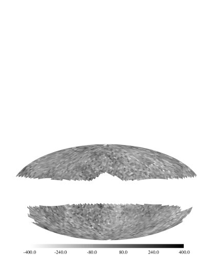
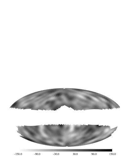
Figure 5: The four-year COBE DMR data are plotted in Aitoff projection. The top panel shows the raw pixel data. The middle panel is the result of filtering the data by removing all but the first 400 signal-to-noise eigenmodes, and the lower panel shows the result of applying a Wiener filter.

The KL expansion is essentially a technique for optimally retaining signal and throwing away noise in a data set. As one might expect, it is closely related to similar methods, such as the Wiener filter (Bunn, Hoffman, & Silk (1996)). Assuming that the statistical properties of the signal and noise are known, applying the Wiener filter to a map preferentially removes noise and leaves signal. It is the optimal linear filter which can be constructed for this purpose.

Wiener filtering is particularly easy to perform in the KL basis. Specifically, the amplitude of the $a$th eigenmode of the Wiener-filtered sky map is obtained simply by multiplying the amplitude of the same mode of the raw map by the eigenvalue $\lambda_{a}$. In Fig. 5 we show the result of Wiener-filtering the DMR data in this way, as well as a map obtained by simply truncating the KL expansion after 400 modes.

3 Frequentist limits

The limits and error bars we have quoted so far in this paper have been based upon Bayesian rather than frequentist techniques. This has become standard practice in CMB data analysis, largely because Bayesian results are often easier to compute than frequentist ones. For a Bayesian, the likelihood function is all that is needed, whereas to find the boundaries of a frequentist confidence interval one also needs to know the theoretical probability distribution of some goodness-of-fit statistic. These probability distributions can often only be computed by time-consuming Monte Carlo simulations.

Although there is nothing intrinsically wrong with Bayesian methods, there are certain circumstances in which a frequentist approach is to be preferred. First, Bayesian estimates may sometimes depend too strongly on the assumed prior, making interpretation of the results controversial. As a rule, this is a serious problem only when the parameter being estimated is weakly constrained by the data (e.g. Bunn et al. (1994)). Second, although Bayesian techniques supply relative probabilities of different models, they are in general unable to determine the intrinsic goodness of fit of a single model. As we saw above, we are able to find the most probable values of parameters like the normalization $Q$ and the spectral index $n$; however, Bayesian methods are unable to tell us whether or not the best fit is actually a good fit.

It is therefore of interest to consider ways of applying frequentist techniques to the COBE data. (We have in fact mentioned some frequentist error estimates above, when we discussed the Monte Carlo simulations we performed to test for bias in our maximum-likelihood parameter estimates.) We begin by reminding the reader of the general approach a frequentist takes to hypothesis testing.

Frequentist statistical analyses are always based on some goodness-of fit statistic $\eta$. The statistic should be chosen in such a way that it takes on low values when the data fit the model well and large values when the fit is poor. For a particular hypothesis, we compute the probability distribution of $\eta$, and we say that the hypothesis is ruled out with significance $s$ if $P(\eta>\hat{\eta})<s$, where $\hat{\eta}$ is the value found in the actual data. For such an analysis to have high power, it is obviously essential to choose $\eta$ wisely.

One common choice of goodness-of-fit statistic is the likelihood ratio. To illustrate this choice, let us consider a family of spatially flat, CDM models with a cosmological constant ($\Lambda$CDM) and $n=1$. These models are characterized on COBE scales by only two parameters, the normalization $Q$ and the density $\Omega_{0}=1-\Omega_{\Lambda}$. If we wish to test the hypothesis that $\Omega_{0}$ takes on some specific value $\Omega_{0}^{*}$, we choose as a goodness-of-fit statistic

$$\eta={\max_{Q,\Omega_{0}}L(Q,\Omega_{0})\over\max_{Q}L(Q,\Omega_{0}^{*})}.$$ (12)

If $\Omega_{0}$ is far from $\Omega_{0}^{*}$, then we expect this ratio to be large. In order to decide whether a particular value of $\Omega_{0}^{*}$ is allowed by the data, we compute the probability distribution of $\eta$ by making many simulated COBE sky maps with a power spectrum corresponding to $\Omega_{0}=\Omega_{0}^{*}$ and computing the likelihood ratio (12) for each one. This time-consuming process must be repeated for each value of $\Omega_{0}^{*}$ we are interested in.

Upon performing this procedure for $\Omega_{0}^{*}=0.1$, we find that the likelihood ratio is 3.16. Only 10% of simulated maps give a larger value, and we therefore conclude that this particular model is ruled out with a significance of 10% (or at 90% confidence). By way of comparison, we shall see below that a Bayesian analysis of the same family of models says that a 95% credible lower limit on $\Omega_{0}$ is 0.13.

Note that this family of models is an example of a situation where the Bayesian limit will have significant prior dependence, since as Fig. 11 shows, the likelihood is large over a significant fraction of the allowed parameter space. A frequentist limit is therefore quite useful. Unfortunately, frequentist limits based on likelihood ratios are extremely expensive to compute, since the probability distribution of $\eta$ must be recomputed by Monte Carlo simulation for each point in parameter space.

The use of likelihood ratios to set frequentist limits alleviates only one of the two disadvantages of the Bayesian approach: we have “removed” the prior dependence, but the likelihood ratio still gives no information about intrinsic goodness of fit: even if the data are an intrinsically poor fit to the whole family of models, there will still be a value of $\Omega_{0}^{*}$ for which the likelihood will peak and $\eta$ will take on its lowest possible value. In (White & Bunn (1995)) we proposed a different goodness-of-fit statistic to resolve this problem, and we will now describe a slight variant of this statistic.

Let $\vec{x}$ be the vector of amplitudes in our eigenmode expansion. For a particular theoretical model, we can compute the theoretical covariance matrix ${\cal M}\equiv\langle\vec{x}\vec{x}^{T}\rangle$, and then transform to a new basis:

$$\vec{y}={\cal M}^{-1/2}\vec{x}.$$ (13)

Any convenient square root of the covariance matrix may be chosen; we recommend Cholesky decomposition. The advantage of changing basis in this way is that the predicted covariance matrix of $\vec{y}$ is the identity matrix. That is, each $y_{i}$ is predicted to be an independent unit Gaussian random variable. We shall see that this can save us a great deal of effort.

Next, we sort the $\{y_{i}\}$ from largest to smallest angular scale probed (by computing the mean value of $\ell$ in a spherical harmonic expansion) and sum $y_{i}^{2}$ over bins of some size $K$:

$$z_{a}=\sum_{i=(a-1)K+1}^{aK}y_{i}^{2},$$ (14)

where $1\leq a\leq N/K$ and $N$ is the total number of modes. If our theoretical model is correct, then each $z_{a}$ should be $\chi_{K}^{2}$-distributed and should therefore have expectation value $K$. If our model is incorrect, then the dispersion of $z_{a}$ about this expectation value should be larger. We therefore propose as a goodness-of-fit statistic the variance,

$$\eta={1\over 2N}\sum_{a=1}^{N/K}(z_{a}-K)^{2}.$$ (15)

The prefactor $1/2N$ is arbitrary; we chose it so that the expectation value of $\eta$ is one when the model is correct.

One great advantage of this statistic is that its probability distribution is model-independent: $\eta$ is simply the average of $N/K$ independent $\chi_{K}^{2}$-distributed random variables. We need to compute this probability distribution only once. Furthermore, unlike the likelihood ratio, this statistic is in principle capable of testing the possibility that the whole family of models under consideration are poor fits to the data.

The statistic (15) has two parameters: the number of modes $N$ and the bin size $K$. We experimented extensively with simulated data sets to find the values of those statistics that maximized the power to reject incorrect models. We made simulated sky maps with a flat $\Omega_{0}=1$ power spectrum and tried to find values of the parameters that maximized our ability to reject an $\Omega_{0}=0.1$ model. We found that the greatest power was achieved when the number of bins was fairly small; we chose $N=200$ and $K=40$, so that the number of bins is only five. Unfortunately, the power of this statistic proves to be quite low: we are typically able to reject the low-$\Omega_{0}$ model with significances of only $\sim 20\%$. As we have seen, the likelihood ratio allows significantly greater power, rejecting the same model at a significance of $10\%$.

It is in general difficult to tell a priori whether a particular goodness-of-fit statistic will be a powerful discriminator among a given class of models; the statistic $\eta$ does not perform as well in this regard as one might have hoped. Although this statistic has low power, it is perhaps nonetheless worth quoting some results based on it, since it is capable of supplying intrinsic goodness-of-fit values for individual models (a task for which the likelihood-ratio is ill-suited). We find that, for the Harrison-Zel’dovich $\Lambda$CDM models we have been considering in this section, the significance ranges from 29% when $\Omega_{0}=1$ to 17% when $\Omega_{0}=0.1$, with higher significances denoting better fits. The fact that all of these significance levels are acceptable is somewhat reassuring: in principle we could have discovered that the whole class of models fit the data at an unacceptably poor level, in which case estimating parameters by means of likelihood ratios or Bayesian methods would be a suspect procedure.

4 Normalization of the Anisotropy Spectrum

We now turn to the problem of quoting the best-fitting amplitude for various models. We break this into two parts: determining the best-fitting amplitude of the radiation power spectrum and the best-fitting amplitude of the matter power spectrum. We discuss the first problem in this section. Since the ratio of the radiation to the matter power spectrum is an output of the model under consideration, the second follows from the first and will be considered in §5.

The inadequacy of using only the RMS fluctuation in the map to determine the amplitude of a given model from has been discussed by (Bunn, Scott & White (1995); Banday et al. (1994); White & Bunn (1995)). As an example, normalizing a scale-invariant Sachs-Wolfe spectrum (Eq. 16) to the RMS anisotropy smoothed to $10^{\circ}$, $\sigma_{10}=29\pm 1\mu$K, one would obtain $10^{11}C_{10}=0.43\pm 0.03$. This is 30% ($\sim 2\sigma$) lower than obtained from a fit to the full data set. However, while the data clearly cannot be summarized by one number, keeping the information from each and every pixel is redundant for the theories we are considering. Since fitting theories directly to the data is quite time consuming, in what follows we will quote results which allow a simple but accurate method for normalizing a given radiation spectrum to the full COBE data.

Figure 6: The angular power spectra $\ell(\ell+1)C_{\ell}$ for CDM models with $\Omega_{\rm B}h^{2}=0.01$, 0.02, 0.03. The tensor power spectrum is also shown. All models are arbitrarily normalized at $\ell=10$. Note that the curves differ significantly, even at low $\ell$, from the flat dashed curve, which represents a pure Sachs-Wolfe spectrum.

Figure 7: The shapes of the angular power spectra are plotted for various CDM models. The upper panel shows spatially flat models with $\Omega_{0}+\Omega_{\Lambda}=1$, and the lower panel shows models with $\Omega_{\Lambda}=0$. All models have $n=1$ and are labeled with the appropriate value of $\Omega_{0}$.

For most models of structure formation the angular power spectrum at low $\ell$ contains little structure. If we could simply parameterize the shapes of the spectra of interest, we could pre-compute and tabulate the normalizations from the COBE data. Which types of spectra should we investigate? As can be seen in Figs. 6 and 7, the radiation power spectrum for a cold dark matter model is not that of a pure Sachs-Wolfe spectrum of gravitational potential perturbations (Abbott & Wise (1984); Bond & Efstathiou (1987); White et al. (1994); Peebles (1993)):

$$C_{\ell}\propto{\Gamma(3-n)\Gamma\left(\ell+{n-1\over 2}\right)\over\Gamma^{2}\left({4-n\over 2}\right)\Gamma\left(\ell+{5-n\over 2}\right)}.$$ (16)

For standard CDM the effect of including the full $C_{\ell}$ spectrum (that is adding the integrated Sachs-Wolfe and velocity contributions) is to reduce the best-fitting normalization by $\sim 10\%$ at $C_{2}$, which gives an indication of the curvature of the spectrum. Including a full numerical calculation of the radiation spectrum also introduces dependences on the cosmological parameters. All except for $\Omega_{0}$ and $n$ are small, as discussed in §5.

We follow (White & Bunn (1995)) in parameterizing the radiation power spectrum in terms of quadratics. Specifically, if we write

$$D(x)=\ell(\ell+1)C_{\ell}\qquad{\rm with}\ x=\log_{10}\ell\quad,$$ (17)

then we provide the normalization for quadratic $D(x)$ using the methods outlined in §2.

To normalize a theory then, one computes the radiation power spectrum for that theory, finds the closest quadratic approximation to it over the range relevant to COBE (roughly $\ell=2$ to $30$) and reads off the normalization which we provide for that quadratic. This works quite well for a large range of theories. For example, for open and $\Lambda$CDM models with $0.2\leq\Omega_{0}\leq 1$ and $0.8\leq n\leq 1.1$ we find at most a 1% difference between normalizing to a quadratic approximation and normalizing to the full theory, as shown in Table 1.

We choose to parameterize the shape of the spectrum by the (normalized) first and second derivatives at $x=1$, specifically $D^{\prime}$ and $D^{\prime\prime}$ where

$$D(x)\simeq D_{1}\left(1+D^{\prime}(x-1)+{D^{\prime\prime}\over 2}(x-1)^{2}\right)$$ (18)

Note that $D^{\prime}$ and $D^{\prime\prime}$ are $1/D_{1}$ times the first and second derivatives of $D(x)$ at $x=1$. The overall normalization is $D_{1}=110C_{10}$. Below we quote the normalization as $D_{1}$ or $C_{10}$, for each $(D^{\prime},D^{\prime\prime})$ pair, and the goodness of fit by the relative likelihood of that shape compared to a featureless, $n=1$, Sachs-Wolfe spectrum: $(D^{\prime},D^{\prime\prime})=(0,0)$.

In terms of this parameterization we find that the following fitting function

$$\ln L = -0.01669+1.19895D^{\prime}$$

$$-0.83527D^{\prime 2}-0.43541D^{\prime\prime}$$

$$-0.03421D^{\prime}D^{\prime\prime}+0.01049D^{\prime\prime 2}$$

describes the likelihood function with an error of 6% in L over the range $-0.6\leq D^{\prime}\leq 0.6$ and $-1\leq D^{\prime\prime}\leq 3$. The peak likelihood is at $(D^{\prime},D^{\prime\prime})=(-0.1,-4)$, which is outside the range of the fitting function, and the likelihood at peak is 8.9 times that for a flat spectrum. The likelihood is plotted as a function of $D^{\prime}$ and $D^{\prime\prime}$ in Fig. 8.

Figure 8: The likelihood $L(D^{\prime},D^{\prime\prime})$ is plotted for power spectra given by Eq. (18). Likelihoods are normalized so that a flat power spectrum ($D^{\prime}=D^{\prime\prime}=0$) has $L=1$, and the contours range from 1 to 8.

Similarly, the best-fitting value of $C_{10}$ is well approximated by

$$10^{11}C_{10} = 0.64575+0.02282D^{\prime}$$

$$+0.01391D^{\prime 2}-0.01819D^{\prime\prime}$$

$$-0.00646D^{\prime}D^{\prime\prime}+0.00103D^{\prime\prime 2}$$

with an error of 1% over the same range. The $1\sigma$ statistical uncertainty in $C_{10}$ is 13.8%. Uncertainties in rms quantities are therefore 7%.

Several popular theories (e.g. open and $\Lambda$CDM models) have radiation power spectra which are not well fit by quadratics all the way down to the quadrupole (e.g. Figs. 6, 7). This is especially true if a tensor component is added since the $\ell=2$ mode is high in the tensor spectrum. While the best-fitting normalization is not too sensitive to the assumption of a quadratic over the entire range, this is not true of the likelihood. We quantify in Fig. 9 and in Table 1 what error in the likelihood function and the normalization arise from approximating several spectra by quadratics. The quadratic approximation causes errors of consistently less than 1% in the normalization $C_{10}$; these errors are completely negligible in comparison with statistical and systematic uncertainties. The errors in the likelihood are somewhat larger, but still not enough to significantly affect our conclusions.

Figure 9: The error in the normalization and the likelihood that arises if a theory which is quadratic in $\ell(\ell+1)C_{\ell}$ for $\ell\geq\ell_{0}$ but constant for $\ell<\ell_{0}$ is approximated by the pure quadratic using the fitting functions Eqs. (19) and (20). The underlying quadratics are taken to be $(D^{\prime},D^{\prime\prime})=$(-0.2,-1; solid), (-0.2,1; dotted), (0.2, -1; short-dashed), (0.2,1; long-dashed).

GW	$\Omega_{0}$	$\Omega_{\Lambda}$	$n$	$\Delta C_{10}$(%)	$\Delta{\cal L}$(%)	GW	$\Omega_{0}$	$\Omega_{\Lambda}$	$n$	$\Delta C_{10}$(%)	$\Delta{\cal L}$(%)
N	0.20	0.80	1.00	0.5	-6	N	0.20	0.80	1.10	0.8	-18
N	0.30	0.00	0.90	-1.2	-14	N	0.30	0.00	1.00	-0.8	-19
N	0.30	0.00	1.10	-0.3	-12	N	0.30	0.70	1.00	0.7	-10
N	0.30	0.70	1.10	0.7	-17	N	0.40	0.60	1.00	0.6	-13
N	0.40	0.60	1.10	0.5	-15	N	0.50	0.50	0.90	0.7	-7
N	0.50	0.50	1.00	0.8	-14	N	0.50	0.50	1.10	0.6	-12
N	0.60	0.00	0.90	0.8	-4	N	0.60	0.00	1.00	0.6	4
N	0.60	0.40	0.90	0.7	-9	N	0.60	0.40	1.00	0.7	-12
N	0.60	0.40	1.10	0.5	-15	N	0.70	0.30	0.90	0.6	-7
N	0.70	0.30	1.00	0.6	0	N	0.80	0.20	0.90	0.7	-9
N	0.80	0.20	1.00	0.6	-9	N	0.90	0.10	0.90	0.6	-9
N	0.90	0.10	1.00	0.6	-10	N	0.90	0.10	1.10	0.3	-14
N	1.00	0.00	0.90	0.6	4	N	1.00	0.00	1.00	0.6	-6
Y	0.30	0.70	0.80	-0.0	20	Y	0.50	0.50	0.80	0.2	11
Y	0.60	0.40	0.80	0.1	21	Y	0.70	0.30	0.80	0.1	31
Y	0.80	0.20	0.80	0.1	19	Y	0.90	0.10	0.80	0.1	13
Y	1.00	0.00	0.80	0.0	34	Y	0.50	0.50	0.90	0.5	5
Y	0.60	0.40	0.90	0.5	7	Y	0.80	0.20	0.90	0.5	20
Y	0.90	0.10	0.90	0.4	13	Y	1.00	0.00	0.90	0.3	11

Table 1: The percentage error introduced by parameterizing theories as quadratics. We have compared the normalization and likelihood for 50 $\Lambda$CDM and OCDM theories with $0.8<n<1.1$ and $0.2\leq\Omega_{0}\leq 1$ as computed using Eqs. (19,20) and directly computed from the data using the numerical power spectrum. Those theories where using the quadratic approximation induces an error of $>0.5\%$ in $C_{10}$ or $>10\%$ in likelihood are shown above. The column labeled GW indicates whether a component of gravity waves was included, as discussed in the text.

The constraints on models from the shape of the COBE power spectrum are not strong. Fig. 10 shows the likelihood function for a family of CDM models in which the density and the cosmological constant are allowed to vary while the spectral index is held fixed. Fig. 11 shows the likelihood function for models with $\Omega_{\Lambda}=0$ and models with $\Omega_{0}+\Omega_{\Lambda}=1$ for three values of the spectral index.

The likelihoods in these figures were computed using the quadratic approximation (18) to the power spectrum rather than the exact power spectrum. The fit to a quadratic is good to $\sim 3\%$ for $\ell\geq 3$, but in the worst cases the error in $C_{2}$ can be as much as 20%. This causes errors of approximately 10-20% in the likelihoods in the worst cases but does not change the general features of the plots.

Figure 10: The likelihood function is shown for a family of CDM models with $n=1$. The likelihoods are normalized so that a flat power spectrum has $L=1$, and the contours are separated by $0.1$ in $L$. The straight dashed line shows the spatially flat models.

Figure 11: Likelihood as a function of $\Omega_{0}$ for CDM models with zero cosmological constant (left) and zero spatial curvature (right). The spectral index $n$ increases from 0.8 to 1.2 from top to bottom. The likelihoods are normalized so that a flat spectrum has $L=1$.

It is clear from these figures that low values of $\Omega_{0}$ are disfavored, especially in the open models. To be more specific, the 95% credible Bayesian lower limit on $\Omega_{0}$ is 0.13 in a scale-invariant ($n=1$) $\Lambda$CDM model, and the 95% credible region for scale-invariant open models is $0.3<\Omega_{0}<1.6$. Both of these limits were computed using a uniform prior in $\Omega_{0}$. In the case of the cosmological constant models, the prior is of course nonzero only when $0<\Omega_{0}<1$.

The low likelihood for low-$\Omega_{0}$ open models comes largely from the shape of the power spectrum at low $\ell$. In fact, a significant portion of our rejection power for these models comes from the quadrupole information. If we exclude the quadrupole from consideration, we find, in agreement with (Górski et al. 1996b ), that we have no 95%-confidence lower limit on $\Omega_{0}$ in a scale-invariant open model. In the case of $\Lambda$ models, excluding the quadrupole weakens the lower limit on $\Omega_{0}$ to about 0.08.

5 Normalization of the Matter Spectrum

5.1 Notation

Until now we have talked about the normalization of the radiation power spectrum on large angular scales. Any theory of structure formation predicts a definite ratio for the normalization of the radiation and matter power spectra. For this reason the COBE DMR detection of CMB anisotropies (Smoot et al. (1992)) allows us to directly normalize the potential fluctuations at near-horizon scales.

For the matter density perturbations, the large-scale structure (LSS) data are usually expressed in terms of the power spectrum $P(k)\equiv\left|\delta_{k}\right|^{2}$, where $\delta_{k}$ is the Fourier transform of the fractional density perturbation

$$\delta_{k}\equiv\delta(|{\bf k}|)=\int d^{3}x\ {\delta\rho\over\rho}\left({\bf x}\right)e^{i{\bf k}\cdot{\bf x}}.$$ (21)

Since standard models postulate Gaussian fluctuations, specifying the power spectrum completely determines the properties of the fluctuations. As the model has no preferred direction, the spectrum depends only on the magnitude of ${\bf k}$. Another measure of $P(k)$ that is often used is the contribution to the mass variance per unit interval in $\ln k$, denoted $\Delta^{2}(k)$, which has the virtue of being dimensionless:

$$\Delta^{2}(k)\equiv{d\sigma^{2}_{\rm mass}\over d\ln k}={k^{3}\over 2\pi^{2}}P(k).$$ (22)

The normalization of $P(k)$ is frequently quoted in terms of

$$\sigma_{8}^{2}\equiv\int_{0}^{\infty}{dk\over k}\ \Delta^{2}(k)\,\left({3j_{1}(kr)\over kr}\right)^{2},$$ (23)

with $r=8\,\,h^{-1}{\rm Mpc}$, which measures the variance of fluctuations in spheres of radius $8\,\,h^{-1}{\rm Mpc}$. Using the Press-Schechter or peak-patch methods, its value can be inferred from the abundance of clusters (Bond & Myers (1991); White, Efstathiou & Frenk (1993); Carlberg et al. (1994); Viana & Liddle (1996); Bond & Myers (1996)) to be $\sigma_{8}\simeq 0.5$–0.8, with some $\Omega_{0}$ dependence. Specifically (Viana & Liddle (1996)) find

$$\sigma_{8}\simeq(0.6\pm 0.1)\Omega_{0}^{-\alpha}\ ,$$ (24)

with $\alpha\simeq 0.4$ for open CDM and $\alpha\simeq 0.45$ for $\Lambda$CDM. (More accurate fits plus a discussion of the uncertainty as a function of $\Omega_{0}$ can be found in their paper.) These values are consistent with those inferred from large-scale flows (Dekel (1994); Strauss & Willick (1995)) and direct observations of galaxies (e.g. Loveday et al. (1992)). Note that for very low $\Omega_{0}$, this implies that optical galaxies become anti-biased (i.e. $b\equiv\sigma_{8}^{\rm gal}/\sigma_{8}<1$).

While $\sigma_{8}$ has been the traditional means of quoting the normalization, COBE probes scales near the horizon size today, so we find it cleanest to quote the normalization in terms of the amplitude of the mass or potential fluctuations at large scales (small $k$). Specifically we use $\delta_{\rm H}$, the density perturbation at horizon-crossing, which is defined through (see e.g. Liddle & Lyth (1993))

$$\Delta^{2}(k)={k^{3}P(k)\over 2\pi^{2}}=\delta_{\rm H}^{2}\left({k\over H_{0}}\right)^{3+n}T^{2}(k),$$ (25)

with $T(k)$ the transfer function describing the processing of the initial fluctuations, which we take to be a power law with index $n$. The relation of the large-scale matter fluctuation amplitude, $\delta_{\rm H}$, to the large-angle radiation anisotropy amplitude, $\sqrt{C_{10}}$, is shown in Fig. 12 and will be discussed more in §§5.3–5.4. In the matter-dominated, critical density, Sachs-Wolfe approximation the proportionality constant in Eq. (16) is simply $(\pi^{2}/8)\delta_{\rm H}^{2}$.

We find to very good approximation that $\delta_{\rm H}$ as determined by COBE is independent of both $h$ and $\Omega_{\rm B}$ (see Figs. 13, 14; for the open models the sensitivity to $h$ is similar to the $\Omega_{0}=1$ case in Fig. 13 while the sensitivity to $\Omega_{\rm B}h^{2}$ is less than in Fig. 14), although it will depend on $\Omega_{0}$ and $\Omega_{\Lambda}$. For definiteness we use $\Omega_{\rm B}h^{2}=0.0125$ and $h=0.75$. For high $\Omega_{\rm B}h^{2}$ and low $h$ one can scale $\delta_{\rm H}$ using Figs. 13, 14.

The value of $\delta_{\rm H}$ is related to the common inflationary amplitude of the scalar perturbations $A_{S}$ (Turner & White (1996); Bunn, Liddle & White (1996)) by $A_{S}\equiv\Omega_{0}/g(\Omega_{0})\times\delta_{\rm H}$, where $g(\Omega)$ is the growth factor discussed in §5.3. When we need to quote the normalization of the tensor (or gravity wave) spectrum independently of the scalars, we shall normalize them to $A_{T}$, where at large scales (Turner & White (1996))

$${d\Omega_{GW}\over d\ln k}\rightarrow{75\over 32}A_{T}^{2}\left({k\over H_{0}}\right)^{-2+n_{T}}$$ (26)

Given $\delta_{\rm H}$, the value of $\sigma_{8}$ can be calculated using Eq. (23). This will introduce an additional dependence on $n$, $\Omega_{0}$, $h$ and the dark matter content of the universe, e.g. $\Omega_{\rm HDM}$. We discuss this in §5.5.

Figure 12: Relation between the normalization of the radiation power spectrum (e.g. $C_{10}$) and the matter power spectrum (e.g. $\delta_{\rm H}$) as a function of $\Omega_{0}$ for CDM models with scale-invariant scalar perturbations.

Figure 13: The power spectrum normalization for scalars (top panel) and tensors (bottom panel) plotted as a function of the Hubble parameter for two flat models. Solid lines in both panels indicate $10^{12}C_{10}$ for the best-fitting scale-invariant CDM model while dashed lines indicate $\delta_{\rm H}$ (top panel) or $A_{T}$ (bottom panel).

Figure 14: The power spectrum normalization for scalar perturbations versus $\Omega_{\rm B}h^{2}$ for two flat models. Solid lines indicate $10^{12}C_{10}$ for the best-fitting scale-invariant CDM model while dashed lines indicate $\delta_{\rm H}$. The sensitivity of the tensors is similarly small.

5.2 Critical Density Models

In the simplest picture, in which large-angle CMB anisotropies come purely from potential fluctuations on the last scattering surface, the relative normalization of the CMB and matter power spectrum today is straightforward (e.g. Efstathiou (1990); White et al. (1994)). In a critical-density universe the potentials are constant in time. If we also assume adiabatic fluctuations, the temperature anisotropy is simply one third of the potential fluctuation, which is related to the density perturbation by the Poisson equation (see White & Hu (1996) for a pedagogical derivation).

For scale invariant scalar fluctuations in a CDM dominated universe with $h=0.5$ and $\Omega_{\rm B}=0.05$ one obtains $\delta_{\rm H}=1.92\times 10^{-5}$. Over the range of scales probed by COBE most models predict spectra which are well approximated by power-laws, so we will allow ourselves to depart from strictly scale-invariant models but keep a power-law initial fluctuation spectrum. The results for tilted ($n\neq 1$) models are a special case of Eq. (29).

In addition to scalar density fluctuations one must consider the possible contribution of gravity waves (tensors) to the COBE fluctuations. If this contribution is non-negligible then the inferred matter fluctuations are correspondingly lower. Conventionally, this is defined in terms of the ratio of tensor to scalar contribution to the quadrupole: $C_{2}^{(T)}/C_{2}^{(S)}$, also written as $T/S$. If the inflationary model is specified then this quantity is calculable, and is related to the tensor spectral index. We shall treat two cases here, that where $T/S=0$ (corresponding to models with a “low” scale of inflation, e.g. Adams et al. (1993); Lyth & Stewart (1996)) and that for which

$${A_{T}^{2}\over A_{S}^{2}}={1-n\over 3-n}$$ (27)

which corresponds to power-law inflation (Lucchin & Matarrese (1985); Lyth & Stewart (1992)). In the $\Omega_{0}=1$ and $n\simeq 1$ limit the above equation reduces to the more familiar $T/S=7(1-n)$ (Liddle & Lyth (1992); Davis et al. (1992); Crittenden et al. (1993); Stewart & Lyth (1993)). More details on the normalization of inflationary models with tensors, and treatment of a wider class of models, can be found in (Bunn, Liddle & White (1996)). For a short discussion of the expectations for the amplitude of the tensor spectrum from the point of view of particle physics models see (Lyth (1996)), and for a review of inflaton potential reconstruction and further relations between observables see (Lidsey et al. (1996)).

Figure 15: The COBE-normalized small-scale fluctuation amplitude $\sigma_{8}$ is plotted for a family of critical CDM models. Solid lines are models with no tensor contribution, and dashed lines have $T/S=7(1-n)$. The hatched region shows the observed value of $\sigma_{8}$ (see text).

Fig. 15 shows the COBE-normalized value of $\sigma_{8}$ for a family of flat CDM models with $\Omega_{0}=1$. While standard $n=1$ CDM predicts an unacceptably large value of $\sigma_{8}$ (unless the Hubble constant is extremely low), even a small amount of tilt is sufficient to bring the prediction in line with the observations.

5.3 Flat Models

There are several additional complications in the case when $\Omega_{0}\neq 1$. Let us first consider models with vanishing spatial curvature, but low $\Omega_{0}$. So we assume that there is a contribution from a cosmological constant which restores spatial flatness: $\Omega_{\Lambda}=1-\Omega_{0}$. In $\Lambda$CDM models the fluctuations stop growing when $z=z_{\Lambda}\sim(\Omega_{0}^{-1}-1)^{1/3}$ for $\Omega_{0}\ll 1$, so the overall growth from $z\sim 10^{3}$ until the present is suppressed by (e.g. Carroll et al. (1992))

$$g(\Omega)={5\over 2}\Omega\left[{1\over 70}+{209\Omega\over 140}-{\Omega^{2}\over 140}+\Omega^{4/7}\right]^{-1}.$$ (28)

In addition, the potential fluctuations are reduced by $\Omega_{0}$. Thus in terms of the power spectrum, $P(k)$, we expect for fixed COBE normalization that $P(k)\propto(g(\Omega_{0})/\Omega_{0})^{2}\sim\Omega^{-1.54}$, as has been pointed out by (Peebles (1984); Efstathiou, Bond & White (1992)). Hence for a fixed COBE normalization the matter fluctuations today are larger in a cosmological constant model than a critical density model.

However, the $g(\Omega_{0})/\Omega_{0}$ behavior is not the only effect which occurs in low-$\Omega_{0}$ universes. Due to the fact that the potentials decay at $z_{\Lambda}$, there is another contribution to the large-angle CMB anisotropy measured by COBE. On large angular scales, i.e., $\ell\lesssim 10$ (Kofman & Starobinsky (1985); Hu & White (1996)), the blueshift of a photon falling into a potential well is not entirely canceled by a redshift when it climbs out, the potential having decayed during transit. This leads to a net energy change, which accumulates along the photon path, often called the Integrated Sachs-Wolfe (ISW) effect to distinguish it from the more commonly considered redshifting which has become known as the Sachs-Wolfe effect (both effects were considered in the paper of Sachs & Wolfe (1967)). Fig. 12 shows the relation between the CMB power spectrum normalization $C_{10}$ and the matter power spectrum normalization $\delta_{\rm H}$. Note that the $g(\Omega_{0})/\Omega_{0}$ scaling of $\delta_{\rm H}$ is fairly accurate for $\Lambda$CDM models where $\Omega_{\Lambda}$ domination occurs late, but less accurate for open models where curvature domination occurs early.

A fit to the four-year COBE data for flat models gives the horizon-crossing amplitude

$$10^{5}\,\delta_{\rm H}(n,\Omega_{0})=1.94\;\Omega_{0}^{-0.785-0.05\ln\Omega_{0}}\exp\left[a\widetilde{n}+b\widetilde{n}^{2}\right]\,,$$ (29)

where $\widetilde{n}=n-1$, $a=-0.95$ and $b=-0.169$ with no gravitational waves, and $a=1$ and $b=1.97$ with power-law inflation gravitational waves. This fit works to better than 3% for $0.2<\Omega_{0}\leq 1$ and $0.7\leq n\leq 1.3$, and again the statistical uncertainty is 7%. For the power-law inflation case the fit is restricted to $n\leq 1$. For $\Omega_{0}\geq 0.3$ there is less than a 5% correction to the $g(\Omega_{0})/\Omega_{0}$ scaling from the ISW component (see Fig. 12).

Figure 16: Contours of $\sigma_{8}$ are plotted for a family of flat CDM models, with $n=0.8$, 1.0 and 1.2. Contours are spaced by 0.25 with the thick solid contour indicating $\sigma_{8}=1$. In all cases $\Omega_{\rm B}h^{2}=0.015$ and we have used the small-scale approximation to the transfer function.

Going to smaller scales, Fig. 16 shows the COBE-normalized value of $\sigma_{8}$ for a variety of flat CDM models.

5.4 Open Models

If we again consider models with low $\Omega_{0}$ but now do not introduce a cosmological constant to restore spatial flatness, we find that keeping track of the ISW effect is extremely important. Even though the calculations become more technically challenging in an open model, it turns out that the largest effect is simple to understand. Since full matter domination occurs so far after last-scattering and curvature domination occurs so early, the gravitational potentials are almost always evolving ($\Phi$ is only constant when the universe is fully matter dominated). For this reason, for the $\Omega_{0}$ of interest in structure formation, the ISW effect dominates the Sachs-Wolfe effect over the entire range of angular scales. Since the temperature anisotropy is enhanced by the ISW contribution, the fluctuations in the matter required to fit COBE are lowered in an open model (see Fig. 12).

There are additional complications due to the curvature selecting a scale in the universe. This means that there is some ambiguity in defining the initial power spectrum. We can obtain some guidance from inflationary open-universe models which predict a nearly scale-invariant spectrum of curvature (or gravitational potential) perturbations, related to density perturbations through the Poisson equation. The density fluctuation spectrum corresponding to a power-law curvature perturbation is (Lyth & Stewart (1990) or see White & Bunn (1995) and references therein)

$$P(k)\propto{(q^{2}+4)^{2}\over q(q^{2}+1)}k^{n-1}$$ (30)

with $q^{2}\equiv k^{2}/(-K)-1$ and $-K=H_{0}^{2}(1-\Omega_{0})$.

In specific open-universe inflationary models based on bubble nucleation there are corrections to this assumption. First $P(k)$ is modified by factors which can enhance or suppress power as $q\rightarrow 0$, typically a factor between $\coth(\pi q/2)$ and $\tanh(\pi q/2)$. Second there is a spectrum of “discrete” modes with $k^{2}<1$ which can add power at small $\ell$, and the fluctuations from the bubble wall can give rise to perturbations in the open universe also (for a readable introduction and overview of open inflationary models, see Cohn (1996)). Furthermore, no calculations have yet been done to asses how good a power-law the initial spectrum is supposed to be in the individual models. Finally there is the possibility that a spectrum of gravitational waves is produced, which should occur if the energy scale of inflation is close to the GUT scale. In short, the theoretical predictions for the power spectra of such models are still quite uncertain.

To avoid detailed modeling of a particular inflationary scenario, we will deal with simple power-law spectra of density perturbations here. For the range of $\Omega_{0}$ of interest the $\coth(\pi q/2)$ and $\tanh(\pi q/2)$ terms do not affect the normalization (Yamamoto & Bunn (1996)). From the point of view of providing a fit to the large-scale structure and CMB data, it appears that low-$\Omega_{0}$ models with a slight spectral tilt $n\sim 1.1$, no super-curvature or bubble wall modes and no tensor component will fit the data best (White & Silk (1996)), thus this assumption combines simplicity with current prejudice. A fit to the four-year COBE data for such models gives the horizon-crossing amplitude

$$10^{5}\,\delta_{\rm H}(n,\Omega_{0})\kern-7.22743pt = \kern-7.22743pt1.95\;\Omega_{0}^{-0.35-0.19\ln\Omega_{0}-0.17\widetilde{n}}$$

$$\exp\left[-\widetilde{n}-0.14\widetilde{n}^{2}\right]\,.$$

This fit works to better than 3% for $0.2<\Omega_{0}\leq 1$ and $0.7\leq n\leq 1.2$, and again the statistical uncertainty is 7%. This $\delta_{\rm H}$ can be used in Eq. (25) for $k\gg\sqrt{-K}$, but note that the behavior of Eq. (5.4) outside the range $0.2<\Omega\leq 1$ is pathological.

Note that the large difference in the scaling with $\Omega_{0}$ between these models and flat models means that the COBE normalization can distinguish open and flat low-density models. The addition of tensor or supercurvature modes would serve only to further suppress the power on small scales in the open models, exacerbating the difference. This means that open models can be distinguished from flat models using the COBE normalization. Fig. 17 shows the COBE-normalized value of $\sigma_{8}$ for a variety of open CDM models. For low $\Omega_{0}$ the scale-invariant models whose shape fits the galaxy clustering data tend to underpredict the cluster abundance (i.e. $\sigma_{8}$) which is the basis of the claim above that models with $n>1$ and no “extra” CMB fluctuations are preferred.

Figure 17: Contours of $\sigma_{8}$ are plotted for a family of open CDM models. with $n=0.8$, 1.0 and 1.2. Contours are spaced by 0.25, increasing to the top right, with the thick solid contour indicating $\sigma_{8}=1$. In all cases $\Omega_{\rm B}h^{2}=0.015$ and we have used the small-scale approximation to the transfer function.

Typically cosmological models are assumed either to be spatially flat or to have vanishing cosmological constant. However, there is no reason in principle not to consider models with both curvature and $\Lambda$. The COBE normalization for scale-invariant models with arbitrary $\Omega_{0}$ and $\Omega_{\Lambda}$ is fit by

$$10^{5}\delta_{\rm H}\kern-7.22743pt = \kern-7.22743pt2.422-1.166e^{\Omega_{0}}+0.800e^{\Omega_{\Lambda}}+3.780\Omega_{0}-$$

$$2.267\Omega_{0}e^{\Omega_{\Lambda}}+0.487\Omega_{0}^{2}+0.561\Omega_{\Lambda}+$$

$$3.392\Omega_{\Lambda}e^{\Omega_{0}}-8.568\Omega_{0}\Omega_{\Lambda}+1.080\Omega_{\Lambda}^{2}$$

to an accuracy of 5% for $0.2\leq\Omega_{0}\leq 1.6$ and $0\leq\Omega_{\Lambda}\leq 0.8$. (For a discussion of such models, especially the closed ones, see White & Scott 1996b .)

5.5 Going to smaller scales

Turning the COBE normalization at the horizon scale into information about clustering of the mass on smaller scales involves the transfer function $T(k)$. Several popular fitting functions exist for $T(k)$ in CDM and mixed dark matter (MDM) models. However, in order to exploit all of the accuracy of the COBE normalization, care must be taken with $T(k)$. As pointed out by (Liddle & Lyth (1993); Peacock & Dodds (1994)) different parameterizations of the transfer function can differ by relatively large amounts. In addition, to obtain accuracy to better than the 10% level, the effect of baryon damping must be included (Peacock & Dodds (1994); Sugiyama (1995); Hu & Sugiyama (1996); Ma (1996); White et al. (1996)).

The MDM power spectrum can be obtained from the CDM power spectrum by multiplying by an additional factor (Pogosyan & Starobinsky (1995); Liddle et al. 1996a ; Ma (1996)). However, no fully satisfactory parameterization of the CDM $T(k)$ has been published. That is to say, no fitting function which is accurate to $\sim 1\%$ over the range $10^{-4}h\,{\rm Mpc}^{-1}\leq k\leq 1h\,{\rm Mpc}^{-1}$ for a wide range of baryon densities (the scaling with the matter density and Hubble constant is $\Omega_{0}h$ so can be included exactly).

Figure 18: A comparison of the numerically evaluated transfer functions (solid squares and open diamonds) with the small-scale approximation discussed in the text (lines). Note that even for extreme parameters the approximation is quite good around $k\sim 0.2h\,{\rm Mpc}^{-1}$ where $\sigma_{8}$ receives its main contribution.

For the purposes of this paper, we shall compute only $\sigma_{8}$. Thus we need an approximation to $T(k)$ which is accurate on small scales. We use the fitting function of (Bardeen et al. (1986)),

$$T_{{\rm CDM}}(q) = \frac{\ln\left(1+2.34q\right)}{2.34q}\times$$

$$\left[1+3.89q+(16.1q)^{2}+\right.$$

$$\left.(5.46q)^{3}+(6.71q)^{4}\right]^{-1/4}\,,$$

with $q=k/h\Gamma$, and $\Gamma$ given by (Hu & Sugiyama (1996), Eq. D-28, E-12). As we show in Fig. 18 this works well even in extreme cases, if one averages over the small ripples inherent in the large $\Omega_{B}/\Omega_{0}$ transfer function. The deviation for $k\geq 0.1h\,{\rm Mpc}^{-1}$ is less than a few percent, though at larger scales it can be significant. The approximation $\Gamma=\Omega_{0}h\exp(-\Omega_{B}-\Omega_{B}/\Omega_{0})$ of (Sugiyama (1995)) works relatively well at large scales for low $\Omega_{B}/\Omega_{0}$ but can lead to unacceptable errors in $T(k)$ outside of this range.

6 Implications for Large-Scale Structure

	$\Omega_{0}$	$\Omega_{\Lambda}$	$\Omega_{\nu}$	$n$	$h$	$\Omega_{\rm B}h^{2}$	$\sigma_{8}$
standard CDM	1.0	0.0	0.0	1.0	0.50	0.0125	1.22
tilted CDM	1.0	0.0	0.0	0.8	0.50	0.0250	0.72
MDM	1.0	0.0	0.2	1.0	0.50	0.0150	0.79
$\Lambda$CDM	0.4	0.6	0.0	1.0	0.65	0.0150	1.07
Open CDM	0.4	0.0	0.0	1.0	0.65	0.0150	0.64
Low $h$ CDM	1.0	0.0	0.0	1.0	0.35	0.0150	0.74

Table 2: Small-scale normalizations for various models.

In principle, COBE lets us constrain models of large-scale structure in two independent ways: we can use both the shape of the power spectrum and the normalization. In practice, though, the shape constraints turn out to be quite weak for most popular models, as we saw in §4 and Fig. 11. We therefore focus on the implications of the power spectrum normalization.

Table 2 gives values of the small-scale density fluctuation amplitude $\sigma_{8}$ for a selection of models. The first line makes it clear that COBE-normalized “standard” CDM ($n=1$, $h=0.5$, $\Omega_{\rm B}h^{2}=0.0125$) predicts significantly too much small-scale power and is therefore ruled out. However, any of several slight changes to the model can easily resolve this inconsistency. Perhaps the simplest solution is a slight tilt to the power spectrum. Inflationary models typically predict spectral indices slightly less than one, and a value of $n$ of 0.8 or even less is quite natural in such models.

We have discussed the difference in normalization between the open and $\Lambda$CDM models in the previous section. By reducing the density we reduce the small-scale fluctuation amplitude as measured, say, by $\sigma_{8}$. Since $\sigma_{8}$ is typically too large in “standard” critical-density CDM models, such low-density models tend to fare better. As we saw above, the suppression of $\sigma_{8}$ is greater in open models than in $\Lambda$CDM models. These results are quantified for some specific models in Table 2.

Another obvious impact of the COBE normalization is that it differentiates between the classes of theories based on adiabatic fluctuations (e.g. inflation) and those based on isocurvature fluctuations (e.g. topological defect models). In the adiabatic models, the fluctuations in all the constituents have the same sign, so an overdensity of photons is also an overdensity of baryons and cold dark matter. This means that photons from overdense regions (which are hotter than average, $n\sim T^{3}$) must climb out of larger than average potential wells, in the process losing energy. In isocurvature models it is “cold” photons which must climb out of such potential wells. Thus, in the adiabatic case the “intrinsic” temperature fluctuation and the gravitational redshifting effect partially cancel, while in the isocurvature case they add. This leads to smaller temperature fluctuations for a given matter fluctuation in the adiabatic case, or conversely larger matter fluctuations when normalized to the temperature fluctuations observed by COBE.

The relative normalization of the matter and temperature fluctuations in any particular model depends upon the details of that model, but the above argument is general enough that we may expect it to hold in a large class of models. Since the adiabatic models predict roughly the right amount of power when compared to large-scale structure measurements on smaller scales, the generic isocurvature models predict too little. These issues are dealt with in more detail in White & Scott 1996a and references therein.

Discussion of particular models of structure formation is beyond the scope of this paper. Analyses based on the four-year COBE data have been performed for critical-density models (White et al. (1996)), $\Lambda$CDM models (Liddle et al. 1996b ), and open CDM models (Górski et al. 1996b ; White & Silk (1996)). The main difference between the four-year results and those based on analyses of the two-year data (e.g., Górski et al. (1995); Stompor, Gorski & Banday (1995); White & Bunn (1995). See also White & Scott 1996a and references therein.) is a reduction of $\sim 10\%$ across the board in the COBE normalizations. Part of this reduction is due to Galactic contamination in the two-year analyses: the two-year data were typically analyzed with a straight $20^{\circ}$ Galactic cut, as opposed to the slightly more extensive “custom cut” (Bennnett et al. (1996)) that has been applied to the four-year data.

7 Conclusions

The four-year COBE DMR sky maps provide some of the most stringent constraints on cosmological models. Because the data are so powerful, and because they are the best large-angle CMB data we are likely to have for the next few years, it is important to extract as much information as possible from them. In particular, when using COBE to normalize models for large-scale structure formation, one should perform a full fit to the data, rather than using a single number such as the root-mean-square temperature fluctuation smoothed on some angular scale.

We have provided normalizations and likelihoods based on the four-year DMR data for a broad class of cosmological models. In conjunction with small-scale measurements of the matter power spectrum such as $\sigma_{8}$, these COBE normalizations allow us to place significant constraints on the parameters of various cosmological models. Furthermore, CMB data on smaller angular scales is improving rapidly in both quality and quantity. By comparing these data with the estimates of the COBE power spectrum, it will soon be possible to severely constrain models on the basis of the CMB angular power spectrum alone.

References

- Abbott & Wise (1984) Abbott, L.F. & Wise, M.B. 1994, ApJ, 282, L47.
- Adams et al. (1993) Adams, F.C., Bond, J.R., Freese, K., Frieman, J.A., Olinto, A.V., 1993 Phys. Rev. D47, 426.
- Banday et al. (1994) Banday, A. et al. 1994, ApJ, 436, L99.
- Banday et al. (1996) Banday, A. et al. 1996, preprint (astro-ph/9601065).
- Bardeen et al. (1986) Bardeen J. M., Bond J. R., Kaiser N., & Szalay A. S. 1986, ApJ, 304, 15.
- Bennnett et al. (1996) Bennett, C.L. et al. 1996, ApJ, 464, L1.
- Bond (1995) Bond, J.R. 1995, Phys. Rev. Lett., 74, 4369.
- Bond & Efstathiou (1987) Bond, J.R. & Efstathiou, G. 1987, MNRAS, 226, 655.
- Bond & Myers (1991) Bond, J. R. & Myers, S., 1991, in “Trends in Astroparticle Physics”, eg. D. Cline and R. Peccei, Singapore, World Scientific, p.262.
- Bond & Myers (1996) Bond, J. R. & Myers, S., 1996, ApJS, 103, 63.
- Bunn (1995) Bunn, E.F. 1995, Ph.D. thesis, University of California, Berkeley.
- Bunn, Hoffman, & Silk (1996) Bunn, E.F., Hoffman, Y., & Silk, J. 1996, ApJ, 464, 1.
- Bunn, Liddle & White (1996) Bunn, E. F., Liddle, A.R., & White, M. 1996, Phys. Rev. D., in press (astro-ph/9607038).
- Bunn, Scott & White (1995) Bunn, E.F., Scott D., & White M. 1995, ApJ, 441, L9.
- Bunn & Sugiyama (1995) Bunn, E. F. & Sugiyama, N. 1995, ApJ, 446, 49.
- Bunn et al. (1994) Bunn, E.F., White, M., Srednicki, M., & Scott, D. 1994, ApJ, 429, 1.
- Carlberg et al. (1994) Carlberg, R. et al., 1994, J. R. Astron. Soc. Canada, 88, 39.
- Carroll et al. (1992) Carroll, S.M., Press, W.H., & Turner, E. L. 1992, ARA&A, 30, 499.
- Cohn (1996) Cohn, J.D. 1996, in “Microwave Background Anisotropies”, Proceedings of the XXXI Moriond Meeting, ed. F. Bouchet., (astro-ph/9606052).
- Crittenden et al. (1993) Crittenden R., Bond J.R., Davies R.L., Efstathiou G., Steinhardt P.J., 1993, Phys. Rev. Lett. 71, 324.
- Davis et al. (1992) Davis, R.L., Hodges H.M., Smoot G.F., Steinhardt P.J., & Turner M.S. 1992, Phys Rev Lett, 69, 1856; erratum ibid 70, 1733.
- Dekel (1994) Dekel, A. 1994, ARA&A, 32, 371.
- Efstathiou (1990) Efstathiou, G., 1990, in “Physics of the Early Universe”, ed. J.A. Peacock, A.E. Heavens & A.T. Davies, Adam Hilger, New York, p..
- Efstathiou, Bond & White (1992) Efstathiou G., Bond J. R., & White S. D. M. 1992, MNRAS, 258, 1P.
- Fixsen et al. (1996) Fixsen, D.J., Cheng, E.S., Gales, J.M., Mather, J.C., Shafer, R.A., & Wright, E.L. 1996, preprint (astro-ph/9605054).
- Górski et al. (1995) Górski, K. M., Ratra, B., Sugiyama, N., & Banday, A. J., 1995 ApJ, 446, L67.
- Górski et al. (1996) Górski, K.M. et al. 1996a, ApJ, 464, L11.
- (28) Górski, K.M. et al. 1996b, preprint (astro-ph/9608054).
- Hinshaw et al. (1996) Hinshaw, G. et al. 1996, ApJ, 464, L17.
- Hu, Bunn & Sugiyama (1995) Hu, W., Bunn, E. F., & Sugiyama, N. 1995, ApJ, 447, L59.
- Hu, Scott & Silk (1994) Hu, W., Scott, D., & Silk, J. 1994, Phys. Rev. D, 49, 648.
- (32) Hu, W., Scott, D., Sugiyama, N., & White, M. 1995, Phys.Rev. D52, 5498.
- Hu & Sugiyama (1996) Hu, W. & Sugiyama, N. 1996, ApJ, in press, (astro-ph/9510117).
- Hu & White (1996) Hu, W. & White, M. 1996, A&A, 315, 33, (astro-ph/9507060).
- Kofman & Starobinsky (1985) Kofman, L. & Starobinsky, A. A. 1985, Sov. Astron. Lett., 9, 643.
- (36) Kogut, A. et al. 1996a, ApJ, 464, L29.
- (37) Kogut, A. et al. 1996b, ApJ, 470, 653.
- Liddle & Lyth (1992) Liddle, A.R. & Lyth, D. 1992, Phys. Lett. B291, 391.
- Liddle & Lyth (1993) Liddle, A.R. & Lyth, D. 1993, Phys. Rep., 231, 1.
- (40) Liddle, A.R. et al. 1996a, MNRAS, 281, 531.
- (41) Liddle, A.R., Lyth, D.H., Viana, P.T.P., & White, M. 1996b, MNRAS, 282, 281.
- Lidsey et al. (1996) Lidsey, J. et al. 1996, Rev. Mod. Phys., in press (astro-ph/9508078).
- Lineweaver et al. (1994) Lineweaver, C.H. et al. 1994, ApJ, 436, 452.
- Loveday et al. (1992) Loveday, J., Efstathiou, G., Peterson, B.A., & Maddox, S.J. 1992, ApJ, 400, L43.
- Lucchin & Matarrese (1985) Lucchin F. & Matarrese S. 1985, Phys Rev, D32, 1316.
- Lyth (1996) Lyth D.H. 1996, preprint, hep-ph/9606387.
- Lyth & Stewart (1990) Lyth D.H., Stewart E. 1990, Phys. Lett. B252, 336.
- Lyth & Stewart (1992) Lyth D.H., Stewart E. 1992, Phys. Lett. B274, 168.
- Lyth & Stewart (1996) Lyth D.H., Stewart E. 1996, preprint, hep-ph/9606412
- Ma (1996) Ma, C.-P. 1996, ApJ, 471, ? (astro-ph/9605198).
- Peacock & Dodds (1994) Peacock, J.A. & Dodds, S.J. 1994, MNRAS, 267, 1020.
- Peebles (1984) Peebles, P. J. E. 1984, ApJ, 284, 439.
- Peebles (1993) Peebles, P. J. E. 1993, “Principles of Physical Cosmology”, (Princeton University Press, Princeton, New Jersey) §21.
- Pogosyan & Starobinsky (1995) Pogosyan, D. & Starobinsky, A. 1995, ApJ, 447, 465.
- Sachs & Wolfe (1967) Sachs, R. K. & Wolfe, A. M. 1967, ApJ, 147, 73.
- Scott, Silk & White (1995) Scott, D., Silk, J., & White, M. 1995, Science, 268, 829.
- Smoot et al. (1992) Smoot, G. et al. 1992, ApJ, 396, L1.
- Stompor, Gorski & Banday (1995) Stompor, R., Gorski, K., & Banday, A. 1995, MNRAS, 277, 1225.
- Strauss & Willick (1995) Strauss, M.A. & Willick, J. 1995, Phys. Rep., 261, 271.
- Stewart & Lyth (1993) Stewart, E. & Lyth, D.H., 1993, Phys. Lett. B302, 171.
- Sugiyama (1995) Sugiyama, N. 1995, Ap.J.Supp, 100, 281.
- Tegmark & Bunn (1995) Tegmark, M. & Bunn, E.F. 1995 ApJ, 455, 1.
- Turner & White (1996) Turner, M. S. & White, M. 1996, Phys. Rev. D53, 6822.
- Viana & Liddle (1996) Viana, P.T.P. & Liddle, A. 1996, MNRAS, 281, 323.
- Vogeley & Szalay (1996) Vogeley, M. S. & Szalay, A. S. 1996, ApJ, 465, 34.
- White & Bunn (1995) White, M. & Bunn, E.F. 1995, ApJ, 450, 477.
- White, Efstathiou & Frenk (1993) White, S.D.M., Efstathiou, G. & Frenk, C. 1993, MNRAS, 262, 1023.
- White & Hu (1996) White, M. & Hu, W. 1996, IAS preprint, (astro-ph/9609105).
- (69) White, M. & Scott, D. 1996a, Comments on Astrophys., 18, 289, (astro-ph/9601170).
- (70) White, M. & Scott, D. 1996b, ApJ, 459, 415.
- White & Silk (1996) White, M. & Silk, J. 1996, Phys. Rev. Lett., in press, (astro-ph/9608177).
- White et al. (1994) White, M., Scott, D., & Silk, J. 1994, ARA&A, 32, 319.
- White et al. (1996) White, M., Viana, P.T.P., Liddle, A. & Scott, D. 1996, MNRAS, in press (astro-ph/9605057).
- Wright et al. (1994) Wright, E.L. et al. 1994, ApJ, 420, 1.
- Yamamoto & Bunn (1996) Yamamoto, K. & Bunn, E.F. 1996, ApJ, 464, 8