Cosmology using the Parkes Multibeam Southern-Sky Hi Survey

Abstract

I discuss the implications of the Parkes Hi Multibeam Southern Sky Survey for cosmology. It will determine the local mass function of Hi clouds, detecting several hundred per decade of mass. Each of these will come with a redshift and, for the more massive clouds, an estimate of the velocity width. This will provide an ideal database for peculiar motion studies and for measurements of biasing of galaxies relative to the underlying matter distribution.

Surveys — Galaxies: luminosity function, mass function — large-scale structure of the Universe

In this paper, I wish to discuss the implications for cosmology of the Parkes Multibeam Southern-Sky Hi Survey (hereafter referred to as ‘the Multibeam Survey’). Most importantly, it will provide the first unbiased survey for Hi clouds, either associated with galaxies or truly isolated: I will show below that many thousand new objects should be discovered whose mass-function will place great constraints on models of galaxy formation. The second important feature of the Multibeam Survey is that it will map the velocity structure of the local Universe in great detail. When combined with accurate Tully-Fisher distances, this will enable strong constraints to be placed on cosmological parameters, principally the density parameter.

1 The mass function of Hi clouds

I will start by estimating the baryonic mass-function of collapsed halos, assuming that baryons and dark matter are distributed equally over the sky (i.e. there is no biasing). I will take parameters appropriate for the standard Cold Dark Matter (CDM) cosmology (others would give similar results): density parameter, $\Omega_{0}=1$; Hubble parameter, $h=H_{0}/100\,$km s^-1Mpc${}^{-1}=0.5$; baryon fraction, $\Omega_{b}=0.064$; normalisation, $\sigma_{8}=0.6$.

An analytic estimate for the number density of halos as a function of mass was first provided by Press & Schechter (1974). To estimate the proportion of the Universe which is contained in structures of mass $m$ at redshift $z$, the density-field is first smoothed with a top-hat filter of radius $R$, where $m=(4\pi/3)\overline{\rho}R^{3}$ and $\overline{\rho}$ is the mean density of the Universe. $F(m,z)$ is then defined to be the fractional volume where the smoothed density exceeds some critical density $\delta_{c}$. Assuming a gaussian distribution, then

$$F(m,z)={1\over 2}{\rm erfc}\left(\delta_{c}\over\sqrt{2}\sigma(m,z)\right),$$ (1)

where $\sigma$ is the root-mean-square fluctuation within the top-hat filter and ${\rm erfc}$ is the complementary error function. The key step was to realize that fluctuations on different mass-scales are not independent. In fact, to a first approximation Press & Schechter assumed that high-mass halos were entirely made up of lower-mass ones with no underdense matter mixed in. Then $F$ must be regarded as a cumulative mass fraction and it can be differentiated to obtain the fraction of the universe contained in structures of a given mass,

$$f(m,z)=-{\partial F\over\partial m}=-{1\over\sqrt{2\pi}}{\delta_{c}\over\sigma^{2}}{\partial\sigma\over\partial m}\exp\left\{-\delta_{c}^{2}/2\sigma^{2}\right\}.$$ (2)

To convert this to a number density of halos per logarithmic mass-interval we simply multiply by $\overline{\rho}$: d$n/$d$\ln m=\overline{\rho}f$. The main drawback of this approach is that, because of the above assumption of crowding together of low-mass halos into larger ones, it seems to undercount the number of objects. However modern techniques (e.g. Bond et al. 1992) give the same analytic form, simply scaled by a factor of two in normalization. The modified formula gives good agreement with numerical simulations (e.g. Lacey & Cole 1994) for $\delta_{c}=1.69$ (as is appropriate for a spherical, top-hat collapse of density peaks.

Figure 1 shows the predicted mass function for the baryonic content of halos and contrasts it with the observed stellar mass function. I have assumed a Schechter luminosity function,

$${\rm d}N={{\cal L}\over L_{*}\Gamma(2+\alpha)}\left(L\over L_{*}\right)^{\alpha}\exp\left\{-L/L_{*}\right\}{\rm d}\left(L\over L_{*}\right),$$ (3)

where ${\cal L}=1.7\times 10^{8}h^{3}\hbox{$\rm\thinspace L_{\odot}$}$Mpc^-3, $L_{*}=10^{10}h^{-2}\hbox{$\rm\thinspace L_{\odot}$}$, $\alpha=-1.25$, and the stellar mass-luminosity ratio is $m_{\rm star}/L=15h$.

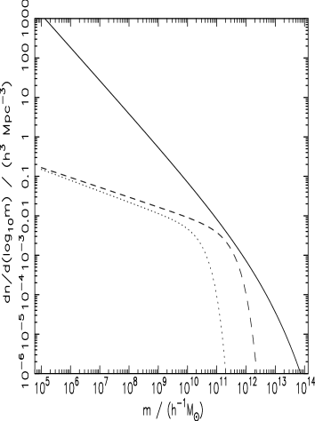
Figure 1: The mass function of halos in the standard CDM cosmology (solid line) compared with the observed luminosity function of galaxies (dashed line) assuming $m/L=15\,h\,\hbox{$\rm\thinspace M_{\odot}$}/\hbox{$\rm\thinspace L_{\odot}$}$. Also shown is the Hi content of normal galaxies (dotted line).

It is apparent that the model predicts approximately the correct number density of normal ($L\sim L_{*}$) galaxies. However, it gives far too many halos at both higher and lower masses. The reason for the former discrepancy was first explained by Rees & Ostriker (1977) and by Silk (1977). They compared the ratio of the cooling time of the gas in proto-galactic halos to the dynamical time of the halo. In small objects the cooling time is always shorter than the dynamical time, thus gas can cool to form stars and hence a visible galaxy. In larger systems, however, the cooling time exceeds the dynamical time. Then mergers may shock-heat the gas before it has time to cool, thus preventing significant star-formation. For this reason clusters of galaxies have little on-going star-formation except perhaps in a cooling flow deep within the cluster core. The dividing mass between these two regimes is highly sensitive to the gas fraction and cooling function but covers the range corresponding to the exponential cut-off in the luminosity function.

The predicted excess of low-mass halos is harder to explain. It would seem that not all the cooled gas in proto-galaxies has formed visible stars. Until I researched this paper, it seemed possible to me that the missing gas resided inside the halos of low-mass galaxies in the form of Hi. The Hi content of normal spiral galaxies is insufficient (see, for example, the mass function shown by the dotted line in Figure 1 which is taken from the model in Briggs 1990) but I thought it possible that there may be a significant population of gas-rich dwarfs. However, the observations of the number counts of Hi clouds, described below, seem to rule this out. This is consistent with the optical luminosity function which, although it may miss many low-surface-brightness, predominantly low-mass galaxies is unlikely to have a faint-end slope as steep as the required value of $\alpha\approx-1.8$. A more realistic explanation for the missing gas is that much of the proto-galactic interstellar medium was heated by an early generation of supernovae (and/or strong galactic winds) and expelled from the halo. If only a small fraction of Hi remains, however, or if it has fallen back into the galaxy, then it should be visible with the Multibeam Survey.

Figure 2 shows the observed number density of Hi clouds in various surveys. The solid data points are taken from Briggs (1990). They all come from pointed observations towards different clusters, but including different proportions of foreground and background objects: solid squares, Leo group (Schneider et al. 1989); circles, Virgo (Hoffman et al. 1989); triangle, Hercules (Salpeter & Dickey 1985). Unfortunately these surveys are all highly biased. The only blind survey for Hi clouds which I know of is that of Kerr & Henning (1987) which has recently been analysed by Henning (1985). That gives a lower space-density as shown by the open squares in the figure. A realistic estimate of the true space-density is probably given by the lower locus of the points in the figure, some one to two orders-of-magnitude below the predicted curve if all the missing matter were in the form of Hi. As the observations must be shifted by about two orders-of-magnitude to the right to give good agreement with the predictions, this suggests that about one percent of the original baryonic mass of the halo persists in the form of Hi.

Figure 2: The detected density of Hi clouds (i.e. galaxies) of different mass, together with the expected sensitivity from the Multibeam Survey. For details see the text.

The dashed line in Figure 2 shows the space density of Hi clouds at which the Multibeam Survey will detect 10 objects of a given mass. The sensitivity is almost three orders-of-magnitude higher than any previous survey thanks mainly due to the large volume of space which is covered. In making this prediction I have have assumed that for a 5 sigma detection

$$m_{\rm H{\sc i}}\geq 2.6\times 10^{7}\hbox{$\rm\thinspace M_{\odot}$}\,\left(D\over 10\,{\rm Mpc}\right)^{2}\left(\Delta v\over 100\,{\rm km}\,{\rm s}^{-1}\right)^{0.5},$$ (4)

where the data have been binned to match the velocity width, $\Delta v$, of the cloud. Supposing one per cent of the baryons to be in the form of Hi, then the Tully-Fisher relation is

$$\Delta v\approx 440\,\left(m_{\rm H{\sc i}}\over 1.5\times 10^{9}h^{-1}\hbox{$\rm\thinspace M_{\odot}$}\right)^{0.22}{\rm km}\,{\rm s}^{-1}.$$ (5)

which gives a minimum density for the detection of $N$ clouds of

$$\phi\geq 1.1\times 10^{-3}\left(N\over 10\right)\left(m_{\rm H{\sc i}}\over 10^{8}h^{-2}\hbox{$\rm\thinspace M_{\odot}$}\right)^{-1.335}h^{0.165}h^{3}\,{\rm Mpc}^{-3}.$$ (6)

The flat part of the sensitivity curve arises for Hi clouds which are detectable to the survey limit of 13 500 km s^-1.

On the basis of Figure 2, I predict that the Multibeam Survey will detect several hundred Hi clouds per decade of mass. I would expect most of these to be associated with dwarf galaxies, but there may be a few truly intergalactic gas clouds. The mass and spatial distribution of these objects will be a major constraint on models of galaxy formation.

2 Numerical simulations of Hi clouds

The formation of bound objects by the growth and collapse of small density fluctuations in the early Universe is a highly complicated process. Although the Press-Schechter formalism, described above, gives a good estimate of the number density of objects, it tells us little about their spatial distribution or their internal structure. For this we have to rely on N-body simulations. Recently there has been a great improvement in the power of such simulations resulting primarily from two causes: firstly the introduction of massively parallel computers consisting of a large number of processors (typically a few hundred) each with their own memory and linked together by high-speed data channels, and secondly the development of sophisticated numerical algorithms able to take advantage of the new machines. Consequently pure N-body simulations (i.e. gravity only, or dark matter only) of a few tens of million particles and N-body, hydrodynamical simulations (i.e. a mixture of gas and dark matter) of a few million particles are now practicable.

Studies of absorption lines in quasar spectra show that the high-redshift Universe is full of Ly$\alpha$ clouds, i.e. clouds of neutral hydrogen. Katz et al. (1995) simulate the production of these clouds in the standard CDM cosmology using parameters similar to those described above. They use 64³ each of dark matter and gas particles with a gas particle mass of $7.75\times 10^{7}h^{-1}\hbox{$\rm\thinspace M_{\odot}$}$. The comoving volume of the box is $11.11\,h^{-1}$Mpc and the box is evolved to a redshift of 2. A uniform photo-ionizing background is assumed to be present since a redshift of 6. Their paper contains a beautiful picture of the surface density of neutral hydrogen at the final time. It shows a dense network of interconnected filamentary structures studded with bright knots representing large concentrations of cold gas. They calculate the optical depth to Hi absorption as a function of frequency for a variety of lines-of-sight through the box. The resultant spectra are then analysed in a similar manner to quasar spectra to produce a histogram of absorption-line equivalent-widths. They are able to to reproduce the general form of the observed distribution over a wide range of equivalent widths, from $10^{14}$–$10^{22}$cm^-2. The low-equivalent-width systems arise from the filaments themselves and from velocity caustics of the gas which is falling onto them. However, the high-equivalent-width systems, $N_{\rm H{\sc i}}\geq 10^{17}$cm^-2, shown in Figure 3, occur when the line-of-sight passes through a lump of collapsed gas, i.e. a galaxy (or more accurately a proto-galaxy as there is no star formation in the code). It can be seen from the figure that the model predicts too few absorption-line systems. This may point to a deficiency in the standard CDM model, but is of little concern to us here.

Figure 3: A histogram of the frequency distribution of Ly$\alpha$ absorbing clouds per line-of-sight ($f(N)=$d${}^{2}N/$d$N_{\rm H{\sc i}}$d$z$) in the numerical simulation of Katz et al. (1995). Error crosses and diagonal boxes show the observational constraints from damped Ly$\alpha$ and Lyman limit systems, respectively.

High-resolution simulations of this kind are very time-consuming and it is impractical to carry them forward beyond a redshift of 2 to the present day. Nor would it be sensible to do so because of all the uncertainties in the physics of the intergalactic medium. However, the Multibeam Survey will anyway only be sensitive to column densities in excess of about $10^{18}$cm^-2 and we have just seen that these are associated with galaxies whose distribution can be determined in simulations of much lower resolution. This is one of the goals of the Virgo Consortium, a collaboration of mainly UK astronomers to carry out cosmological N-body hydrodynamical simulations of the formation of structure. We have been awarded time on the Cray T3D supercomputer at Edinburgh that consists of 512 Dec alpha chips (of which 256 are usable at one time) each with 64 Mb of memory. We use the Hydra code developed by Couchman, Thomas & Pearce (1995) and available from http://coho.astro.uwo.ca/pub/hydra/hydra.html. Currently we are carrying out dark matter simulations with 17 million particles and dark matter plus gas simulations with 4 million particles. Only the latter are of relevance for this paper.

Figure 4 shows the distribution of cold gas ($T<10^{5}$K) in one of our simulations at $z=0$. It is a slice $7\,h^{-1}$Mpc thick through a box $70\,h^{-1}$Mpc in width. The cosmological parameters are again similar to those given above, but the particle mass is now $1.4\times 10^{9}h^{-1}\hbox{$\rm\thinspace M_{\odot}$}$. The box-size is well-matched to the size of the Multibeam Survey, although the mass-resolution is poorer than one would like and allows us to model the distribution of only the more massive galaxies. However, I would expect an improvement of a factor of eight in mass-resolution within a couple of years. If one looks carefully then one can see numerous lumps of cold gas spaced along and at the intersection of filaments: these we associate with galaxies. It should be noted, however, that we have deliberately kept the physics in these simulations to a minimum. In particular, we have not attempted to form stars with all the associated feedback of energy into the interstellar medium. For this reason the Hi mass in the simulations is not representative of that in real galaxies.

One of the main purposes of including gas in the simulations is to test the bias in the relative distributions of galaxies and dark matter. The former are more highly-correlated in space and are also moving more slowly than the latter. Moreover, the degree of biasing is dependent upon the mass of the galaxies, being larger for more massive systems. As an illustration of this, Figure 5 shows the relative distributions of moderate and high-mass galaxies in a test simulation. It will be very interesting to see from the Multibeam Survey whether there is a large population of dwarf galaxies filling the voids in the bright galaxy distribution.

Figure 5: Projections of the galaxy distribution in a test simulation: (a) $m<0.5M_{*}$, (b) $m>0.5M_{*}$, where $M_{*}=1.5\times 10^{11}h^{-1}\hbox{$\rm\thinspace M_{\odot}$}$.

The degree of biasing is a major bug-bear of cosmology because it confuses the link between observations and theory: we see the galaxies, but the models predict only the overall distribution of matter. For example, one of the best ways to estimate the density parameter, $\Omega_{0}$, is to measure the peculiar velocities of galaxies relative to the uniform Hubble expansion. The expected motions are proportional to $\Omega_{0}^{0.6}$ and also to the overdensity of matter, that is $1/b$ times the overdensity of light where $b$ is the bias parameter. The Multibeam Survey will be an ideal database for peculiar motion studies. As well as detecting all large spiral galaxies out to more than $100\,h^{-1}$Mpc, it will also measure their redshift and their Hi velocity width. When combined with infra-red photometry, this latter quantity will enable accurate Tully-Fisher distances and hence peculiar velocities.

Figure 6 shows ‘wedge diagrams’ for the real and velocity space distribution of galaxies drawn from an N-body simulation with $\Omega=0.3$ and extent similar to the Multibeam Survey. The high density of galaxies which is expected in the Multibeam Survey provides an advantage over other sparser surveys: if one can find a well-defined void similar to those seen in the figure, then one can obtain a constraint on $\Omega_{0}$ which is independent of the bias parameter. This is because the underdensity in a void can never be greater than unity (whereas the overdensity in a cluster can in principle be anything).

Figure 6: ‘Wedge diagrams’ for the galaxy distribution in a simulation of spatial extent similar to the Multibeam Survey: (a) redshift space, (b) real space.

3 Conclusions

1. The Parkes Multibeam Hi Southern Sky Survey will determine the mass function of Hi clouds in the local Universe. This will provide a strong constraint on models of galaxy formation.

2. The spatial distribution of Hi clouds of differing mass will test ideas about biasing in the galaxy distribution.

3. A complete survey of high-mass galaxies, plus Tully-Fisher estimates of distances and hence peculiar velocities, will provide strong constraints on the density parameter.

Acknowledgments

I would like to acknowledge the support of a Nuffield Foundation Science Research Fellowship and the hospitality of the University of Melbourne where the preparation of this paper was undertaken. Thanks also to David Weinberg for supplying me with a copy of Figure 3.

Bond J. R., Cole S., Efstathiou G., Kaiser N., 1992, ApJ, 379, 440

Briggs F. H., 1990, AJ, 100, 999

Couchman H. M. P., Thomas P. A., Pearce, F. R., 1995, 452, 797

Henning P. A., 1995, ApJ, 450, 578

Hoffman G. L., Lewis B. M., Helou G., Salpeter E. E., Williams H. L., 1989, ApJS, 69, 65

Katz N., Weinberg D. H., Hernquist L., Miralda-Escudé J. M., 1995, preprint, astro-ph/9506106

Kerr F. J., Henning P. A., 1987, 320, L99

Lacey C. G., Cole S., 1994, MNRAS, 271, 676

Press W. H., Schechter P. G., 1974, ApJ, 187, 425

Rees M. J., Ostriker J. P., 1977, MNRAS, 179, 541

Salpeter E. E., Dickey, J. M., 1985, ApJ, 292, 426

Schneider S. E. et al. , 1989, AJ, 97, 666

Silk, J., 1977, ApJ, 211, 638