The shape of the ionizing UV background at $z\sim 3.7$ from the metal absorption systems of Q$0000-2619$

Abstract

Spectra of the $z_{em}$$=4.12$ quasar Q$0000-2619$ have been obtained in the range $\lambda\lambda=4880-8115$ Åwith a resolution of 13 kms^-1and signal–to–noise ratio of $s/n=15-60$ per resolution element. The list of the identified absorption lines is given together with their fitted column densities and Doppler widths. The mode of the distribution of the Doppler parameters for the Ly$\alpha$lines is $\simeq 25$ kms^-1. The fraction of lines with $10<b<20$ kms^-1is 17%. The Doppler values derived from uncontaminated Ly$\beta$lines are smaller than those obtained from the corresponding Ly$\alpha$ lines, indicating the contribution of non saturated, non resolved components in the Ly$\alpha$profiles.

The integrated UV background estimated from the proximity effect is found to be $J\sim 7\times 10^{-22}$ erg s^-1 cm^-2 Hz^-1 sr^-1. This value is consistent with previous estimates obtained at a lower $z$, implying no appreciable redshift evolution of the UVB up to $z=4$.

13 metal systems are identified, five of which previously unknown. The analysis of the associated metal systems suggests abundances generally below the solar value with an average [C/H] $\sim-0.5$. This value is about one order of magnitude higher than that found in intervening systems at about the same redshift.

The analysis of the intervening metal line systems has revealed in particular the presence of three optically thin systems with $\log N_{HI}\sim 15$ showing associated CIV and SiIV absorptions. In order to make the observed column densities consistent with [Si/C] ratios lower than 10 times the solar value, it is necessary to assume a large jump in the spectrum of the ionizing UV background beyond the HeII edge ($J_{912}/J_{228}\ \raise-2.0pt\hbox{\hbox to0.0pt{\hbox{$\sim$}\hss}\raise 5.0pt\hbox{$>$}\ }1000$). This result, if confirmed in other spectra at the same redshift is suggestive of a possible dominance of a stellar ionizing emissivity over the declining quasar one at $z>3$.

Key words: Galaxies: formation of – general: intergalactic medium – quasars: Q$0000-2619$

1 Introduction

Table 1.: Log of the observations.

setup	No.	date	range	FWHM	grating	CD	slit	exposure
	of spectra		(Å)	(Å)		grism	width	(s)
E1	2	15/10/90	$4700-6452$	0.2	10	#5	1.2”	5400/6600
E2	2	18/10/90	$5830-8550$	0.3	10	#4	1.2”	4200/5100
E3	3	24-25/11/94	$4820-8450$	0.3	10	#3	1.25”/1.25”/1.3”	5000/5600/5000
G1	2	26-27/11/95	$4000-10000$	10	–	#1	5”/1.5”	900/900

The Ly$\alpha$forest detected in the blue side of the quasar Ly$\alpha$emission is generally ascribed to an intergalactic population of hydrogen clouds. Ly$\alpha$clouds are present at all the observed redshifts from the largest to the present epoch, (e.g. Carswell 1995; Bahcall et al. 1996; Giallongo et al. 1996), covering a substantial fraction of the total age of the universe. The origin and evolution of the clouds are intimately linked with the physical conditions and evolution of the universe (Miralda-Escudé et al. 1996). While the strongest Ly$\alpha$clouds showing associated metals are thought to be associated with intervening galaxy halos (Bergeron & Boissé 1991; Bergeron et al. 1992; Steidel et al. 1994), the environment of the optically thin ones is less clear. At least at low redshift some Ly$\alpha$with column densities $\ \raise-2.0pt\hbox{\hbox to0.0pt{\hbox{$\sim$}\hss}\raise 5.0pt\hbox{$>$}\ }10^{14}$ cm^-2 have been associated with the external parts of galaxy halos (Lanzetta et al. 1995).

There are however recent observational suggestions indicating a continuity scenario between Ly$\alpha$lines with $\log N_{HI}\ \raise-2.0pt\hbox{\hbox to0.0pt{\hbox{$\sim$}\hss}\raise 5.0pt\hbox{$>$}\ }14$ and the stronger metal line systems. Clustering of the Ly$\alpha$clouds has been found up to scales of 300 kms^-1(Cristiani et al. 1995,1996; Chernomordik 1995; Hu et al. 1995; Fernandez–Soto et al. 1996) with an amplitude increasing with $N_{HI}$. In particular, Cristiani et al. 1996 found that an extrapolation of this trend to $\log N_{HI}\sim 17$ is consistent with the corresponding estimate derived from the CIV metal systems by Petitjean & Bergeron 1994.

Weak CIV lines have been found to be associated with Ly$\alpha$lines with $\log N_{HI}=14.5\sim 15$ (Cowie et al. 1995; Tytler et al. 1995) with abundances similar to that of the metal line systems.

Disentangling between different scenarios for the cloud structure and their cosmological evolution requires a large database of high resolution spectra. The sample available in literature is still limited, but new impulse in the field has come from the observations with the HIRES spectrograph at the Keck telescope (Cowie et al. 1995; Hu et al. 1995)

Within an ESO Key Project on intergalactic matter at high redshift, we have obtained at the 3.5m NTT high resolution spectra of several QSOs at redshift larger than 3 (Giallongo et al. 1996). We present and discuss here in detail data on the Ly$\alpha$forest and the metal systems of the QSO $0000-26$ ($m_{R}=17.5$, $z_{em}=4.12$). The spectra cover the range 4880 to 8115 Åat a resolution of 13 kms^-1. A preliminary investigation of the spectrum of Q$0000-26$ in the range 4700 to 6600 Å at a resolution of 30 kms^-1has been reported by Webb et al. 1988. A first discussion of the metal systems in Q$0000-26$, based mainly on the data in the spectral region around the Ly$\alpha$ emission and to the red of it, has been given by Savaglio et al. 1994, while a detailed study of the metallicity of the damped Ly$\alpha$system at $z=3.39$ has been reported by Molaro et al. 1995.

In this paper we present in section 2 the observations, the data reduction procedure and the list of the Ly$\alpha$lines and identified metal lines with the fitting parameters column density, Doppler width and redshift. The result of the statistical analysis of the Ly$\alpha$forest is presented in section 3. The metal line systems are discussed in section 4.

2 Observations and data extraction

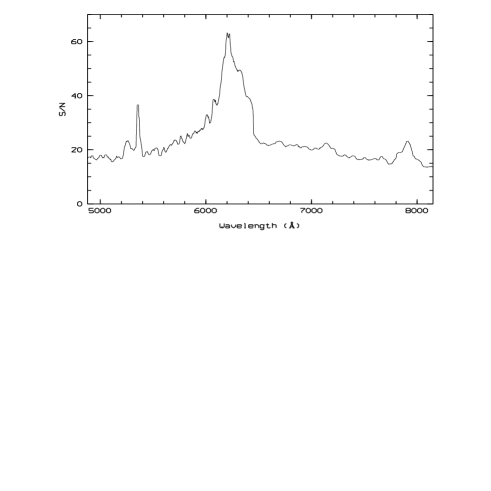
Fig. 1.: Signal–to–noise ratio per resolution element as function of wavelength in the spectrum of Q$0000-26$.

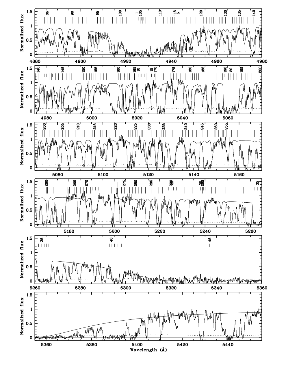
Fig. 2.: Absorption lines of Q$0000-26$. The normalized spectrum is shown as full line, the fit as thin line and the noise per pixel as dashed line. Long ticks correspond to Ly$\alpha$and Ly$\beta$lines, short ticks correspond to metal lines. For $\lambda<5260$ Åthe Ly$\beta$lines are indicated with the same number as the corresponding Ly$\alpha$lines.

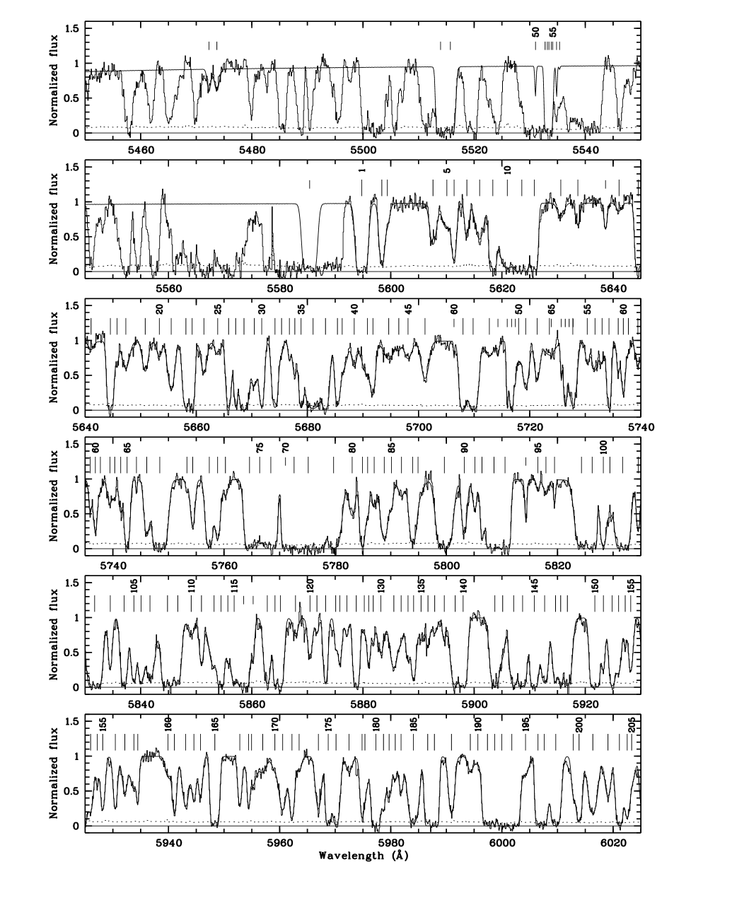
Fig. 2.: – Continued

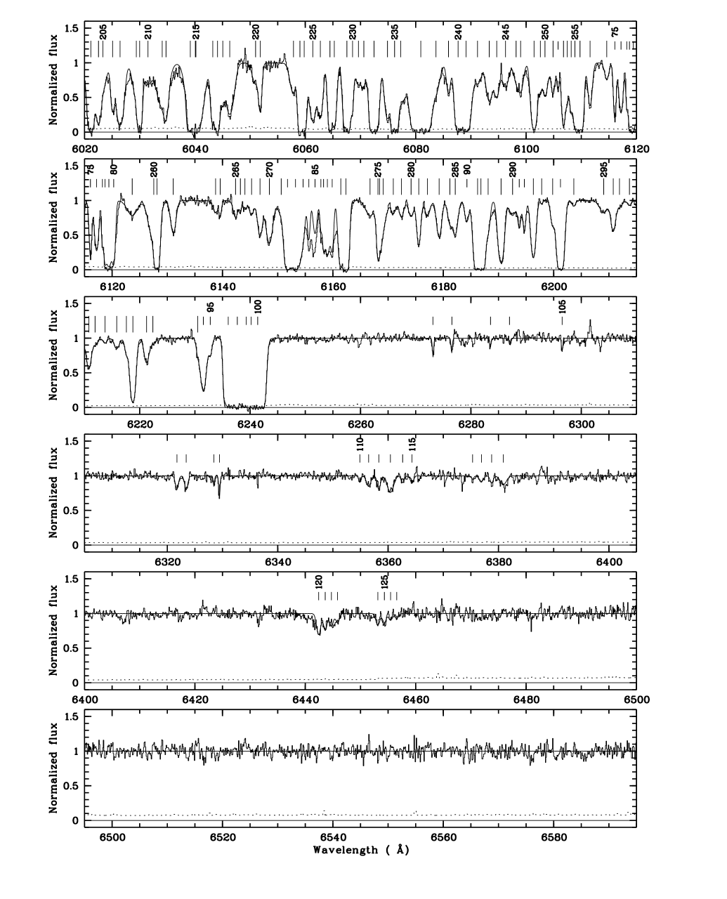
Fig. 2.: – Continued

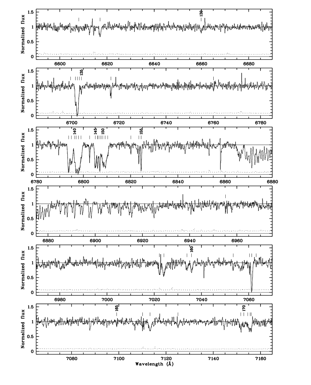
Fig. 2.: – Continued

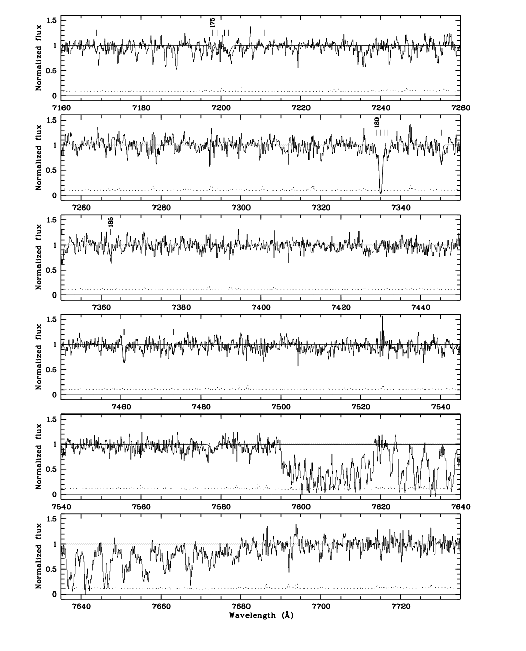
Fig. 2.: – Continued

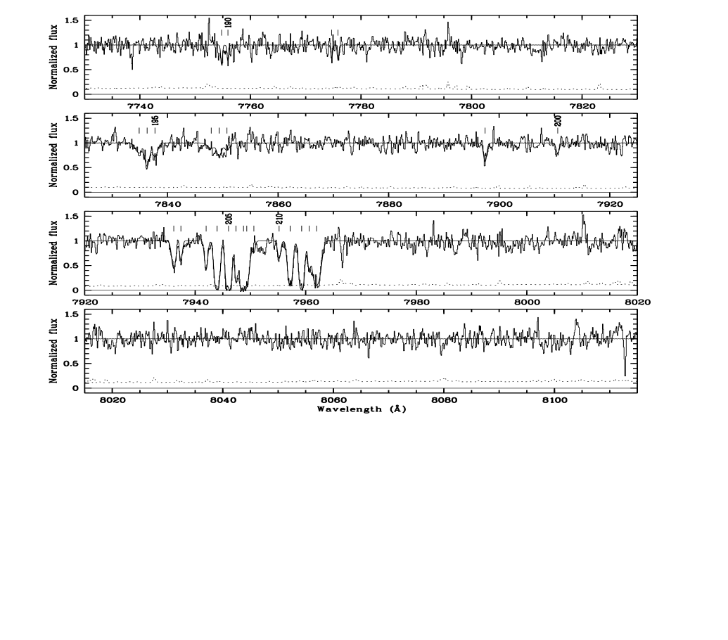
Fig. 2.: – Continued

The echelle observations of Q$0000-2619$ presented here were obtained with the EMMI instrument (D’Odorico 1990) at the ESO NTT telescope in October 1990 and November 1994. The log of the observations is given in Table 1. The second column gives the number of individual spectra obtained with each setting. The seeing during the observations was typically between 0.8 and 1.2 arcsec.

The absolute flux calibration was carried out by observing of the standard stars Feige 110 (Stone 1977), LTT7987 (Stone and Baldwin 1983 and Stone and Baldwin 1984) and HD49798 (Walsh 1992).

The echelle data were reduced with the ECHELLE software package available in the MIDAS software. The wavelength calibration spectra of the Thorium-Argon lamp were extracted in the same way and used to establish the wavelength scale. Wavelengths have been corrected to vacuum heliocentric values. The weighted mean of the spectra has been obtained at the resolution of about $R=24000$. The variance spectrum was obtained by propagation of the photon statistics of the object and sky spectra, and from the detector read–out–noise. The final signal–to–noise ratio per resolution element is shown in Fig.1.

The normalized spectrum is plotted in Fig.2 in the wavelength interval $\lambda\lambda=4880-8115$ Å. The dedicated software FITLYMAN (Fontana & Ballester 1995) in the MIDAS package was used to derive the redshift $z$, the Doppler parameter $b=\sqrt{2}\sigma$ and the column density $N$ of the absorption lines. The line fitting has been performed by a $\chi^{2}$ minimization of Voigt profiles, after deconvolution with the instrumental profile.

Despite the high resolution, most of the features appears to be strongly blended, contrary to what is found in lower $z$ QSOs, where the lines are typically isolated. As in previous similar analyses (e.g.Giallongo et al. 1993), complex structures have been fitted with the minimum number of components required to give a probability of random deviation $P>0.05$.

We performed the fitting of all the line complexes in the region with $s/n\ \raise-2.0pt\hbox{\hbox to0.0pt{\hbox{$\sim$}\hss}\raise 5.0pt\hbox{$>$}\ }20$, i.e. from $z=3.602$, to the quasar Ly$\alpha$emission line ($\lambda\lambda=5590-6240$ Å).

The parameter list for about 300 Ly$\alpha$lines is reported in Table 2, while Table 3 lists the metal lines. Only the fitted lines appear in the tables.

The position of fitted lines is marked on the top of Fig.2 with the numbering as given in Table 2 and 3. Long ticks show Ly$\alpha$lines (Table 2) and with the same numbering the associated Ly$\beta$lines in the wavelength range $4880-5260$ Å. Short ticks are metal absorption lines (Table 3).

The Ly$\alpha$forest is contaminated by the metal lines of two damped Ly$\alpha$systems and other 11 metal systems, 4 of which with $z_{abs}$$\approx$ $z_{em}$. In Table 3 the Ly$\alpha$lines associated with metal systems are indicated as “MLy$\alpha$” and taken off from the sample used for Ly$\alpha$analysis and statistics.

A low resolution ($R=280$) spectrum of Q$0000-26$, covering the range $\lambda\lambda=4000-10000$ Å, has been obtained in the long slit mode of EMMI at the NTT in November 1995 (see Table 1). The absolute flux calibration was carried out observing the standard star Feige 110.

3 The Ly$\alpha$forest

Clues on the physical nature of Ly$\alpha$clouds may be obtained from the statistical distributions of their parameters (redshift, Doppler width and column density) obtained through line profile fitting.

The present data, covering a wide redshift range with good signal–to–noise, are especially suited to address the issue of the Doppler parameter distribution and to study the UV background at $z\sim 3.5-3.8$. The redshift evolution and column density distribution of the Ly$\alpha$clouds have been already discussed using a larger data base in Giallongo et al. (1996).

3.1 The Doppler parameter distribution

While it is generally agreed that “typical” Ly$\alpha$clouds have Doppler parameters of the order of $b\sim 25$ kms^-1, the actual fraction of narrow ($b<20$ kms^-1) and broad ($b>50$ kms^-1) lines is more difficult to determine, because of the possible systematic effects involved.

Large $b$ values may be a result of the intrinsic difficulty in finding out sub-components in blends, while noise effects and the contamination of unrecognized metal lines may increase the fraction of narrow lines (Rauch et al. 1993).

The strong biases in the detection and measure of the narrow lines can be minimized with high quality data on an extended redshift range, as in the present spectrum. As shown in Fig.3, low $b$ values are not correlated with the wavelength and consequently with the $s/n$ (see also Fig.1).

The Doppler parameter distribution has been obtained by selecting all the lines out of 8 Mpc from the QSO, not affected by the proximity effect, and is shown in Fig.4.

As usual, the distribution appears skewed towards large $b$ values. The mode of the distribution is 25 kms^-1and 17% of the lines have $10<b<20$.

To estimate the intrinsic dispersion of the distribution we calculate iteratively the mean $b$ value excluding lines with 2$\sigma$ beyond the mean. In this way we avoid large, possible spurious $b$ deriving a mean value $\langle b\rangle=26$ kms^-1and $\sigma_{b}=8$ kms^-1. The distribution of measurement errors has a median value $\simeq 3$ kms^-1so does not affect appreciably the observed $b$ dispersion. After subtraction in quadrature we obtain $\sigma_{b}=7$ kms^-1.

Of course any intrinsic $b$ distribution with an artificial cutoff at the low end produces a low$-b$ tail due to measurement errors (Hu et al. 1995). A very large statistics with low measurement errors is needed to deconvolve the intrinsic distribution from the observed one. Without a very large Ly$\alpha$sample, the problem of the intrinsic fraction of narrow lines remains an open question although photoionization models (Giallongo & Petitjean 1994; Ferrara & Giallongo 1996) and recent cosmological models for the Ly$\alpha$clouds (Hernquist et al. 1996; Miralda–Escudé et al. 1996) are able to produce $b$ values as low as $b\sim 15$ kms^-1.

3.2 The Ly$\beta$forest and the $b$ values

Fig. 3.: The Doppler parameter $b$ as function of wavelength.

Table 2.: Absorption line parameters of the Ly$\alpha$forest. Lines marked with an asterisk have been fitted using simultaneously the observed Ly$\alpha$and Ly$\beta$profile.

Table 2.: – Continued

Table 3.: Absorption line parameters of the metal systems.

Table 3.: – Continued

The line parameters derived from Ly$\alpha$fitting have been compared with the corresponding Ly$\beta$lines. In general the Ly$\beta$forest is mixed with the Ly$\alpha$forest at lower $z$, but in several cases we found isolated absorptions in correspondence of the position of the expected Ly$\beta$. For these systems we tried a simultaneous fit for the Ly$\alpha$and Ly$\beta$components of the same cloud. Since the Ly$\beta$line in these cases is less saturated than the corresponding Ly$\alpha$, a more accurate estimate of $N_{HI}$ and $b$ is obtained. In Fig.5 we show a sub-sample for which the Ly$\alpha$+Ly$\beta$fit gives a significantly different result from the fit with only the Ly$\alpha$component. In general the high column density Ly$\alpha$lines tend to split in more components: the initial 13 lines become 22 after decomposition. These 22 lines are marked with an asterisk in Table 2. Besides the $b$ mean value goes from 43 kms^-1to 28 kms^-1in better agreement with the $b$ distributions derived in Sect 3.1 and by Hu et al. (1995).

While a firm statistical conclusion cannot be drawn with these few cases, they suggest that at least some of the lines with large $b$ are due to blends of several components. In this way the tendency of lines with larger $b$ to show larger column densities is strongly reduced.

3.3 The UV background at $z\ \raise-2.0pt\hbox{\hbox to0.0pt{\hbox{$\sim$}\hss}\raise 5.0pt\hbox{$<$}\ }4$

Fig. 4.: The Doppler parameter distribution, with a median value of about 27.8 kms^-1. The lines are those not affected by the proximity effect.

Fig. 5.: Plot of the Doppler parameter $b$ versus $\log N_{HI}$ for a subsample of absorption lines. Solid dots are parameters obtained from a fit of the Ly$\alpha$only, the squares show the result of the fit when Ly$\beta$is also considered. One can note a splitting of the higher column density lines and a lowering of the $b$ values.

Fig. 6.: $\partial n/\partial X_{\gamma}$ as function of $\log\omega$ for lines with $\log N_{HI}\geq 13.8$ and for the UV background radiation $J\simeq 7\times 10^{-22}$ erg s^-1 cm^-2Hz^-1 sr^-1.

The reduction of the number density of the absorption lines along the wing of the quasar Ly$\alpha$emission is interpreted as due to the enhancement of the ionization of the gas cloud by the UV emission of the nearby quasar which is superimposed to the general UV background (Bajtlik et al. 1988). This proximity effect allows a statistical estimate of the UVB as a function of redshift.

Following the Bajtlik et al. model, the line distribution per unit column density can be represented in the proximity of the QSO by (the subscript HI is omitted for simplicity):

$$\frac{\partial^{2}n}{\partial z\partial N}=A(1+z)^{\gamma}N^{-\beta}(1+\omega)^{(1-\beta)}\penalty 10000\kern 3.0pt.$$ (1)

where $\omega$ is the ratio of the quasar Lyman limit flux to the background flux received by any cloud at its redshift.

Assuming a power law spectrum $f_{\nu}\propto\nu^{-\alpha}$, with $\alpha=0.72$ (Schneider et al. 1989) and the continuum flux estimated at the minimum between SiIV and CIV emissions from the spectrum of Schneider et al. 1989, the flux at 912 Åis $f_{912}=2.5\times 10^{-27}$ erg s^-1 cm^-2Hz^-1. Uncertainties in the calculation of $\omega$ depend mainly on the estimate of the systemic emission redshift of the quasar. As shown by Espey et al. (1993), the best estimate of the actual redshift is given by the low ionization lines, as for example the MgII doublet. We adopted the value $z_{em}=4.126$ as we derived from the fit to the OI(1302) emission line.

We have considered the sample of Ly$\alpha$lines not associated with metal systems with $z\geq 3.60$ and $\log N_{HI}\geq 13.8$. The high threshold adopted for the column density of the sample avoids the bias in the redshift distribution of the weaker lines due to the blanketing effect produced by the stronger ones.

In Fig.6 the predicted distribution of the line density in the coevolving redshift interval $dX_{\gamma}=(1+z)^{\gamma}$ is shown together with the data points binned as in Bajtlik et al. (1988). The best fit gives $J=J_{-22}\times 10^{-22}$ erg s^-1 cm^-2Hz^-1 sr^-1 with $J_{-22}\simeq 7$ assuming an intrinsic line distribution with $\gamma=2.89$, $\beta=1.79$ and $A=10^{11.22}$, as derived from the statistical analysis of the data sample used by Giallongo et al. (1996) for lines with $\log N_{HI}\geq 13.8$. Only values $J_{-22}<4$ and $J_{-22}>18$ are excluded at more than 2$\sigma$ level. This result is consistent with the value $J_{-22}=6$ derived from a large data sample (including this spectrum) by Giallongo et al. (1996) without correction for line blanketing. Including line blanketing corrections in the large sample reduces the UVB from $J_{-22}=6$ to $J_{-22}=5$. At higher redshift, $z\sim 4.5$, Williger et al. (1994), have measured the proximity effect in the forest of BR$1033-03$ obtaining a value $J_{-22}\sim 3$. This might imply a possible evolution of the UVB at $z>4$, which is to be confirmed by a larger data set.

The value derived from the proximity effect in Q$0000-26$ is not far from that predicted for the quasar population at the same redshift $J_{-22}\sim 1-2$ (Haardt & Madau 1996), although there is room for a contribution by other kind of ionizing sources like primeval galaxies.

Disentangling between these two possibilities requires the knowledge of the shape of the UV background around the HeII edge at 4 Rydberg (228 Å). This can be done either through the direct measure of the quasar flux at 4 $Ryd$ in the few cases where the quasar spectrum can be observed in this region (Jakobsen et al. 1994; Davidsen et al. 1995) or in an indirect way through the measure of the relative abundances of ions like CIV and SiIV whose ionization potentials are near the HeII edge (Miralda-Escudé & Ostriker 1990). In the next section we derive constraints on the shape of the UVB and on the nature of the ionizing sources from the study of three optically thin Ly$\alpha$absorption systems at $z\ \raise-2.0pt\hbox{\hbox to0.0pt{\hbox{$\sim$}\hss}\raise 5.0pt\hbox{$>$}\ }3.5$.

4 The metal systems

The metal systems of $0000-26$ have been already studied in Savaglio et al. (1994). In this work, the new data allow to confirm the old metal systems (except one) and to identify five new ones, with relatively low HI column density. Table 4 lists the two low redshift metal systems containing the MgII absorption doublet. Table 5 shows the CIV high-redshift systems with $z_{em}-z_{abs}>5000$ kms^-1, considered to be intervening. Table 6 lists the CIV systems with $z_{em}-z_{abs}<5000$ kms^-1, considered to be associated. All the high-redshift systems show CIV doublet together with the Ly$\alpha$line.

For all the systems we looked for metal lines of cosmological relevance falling in the observed range. For most of these, we give upper limits to the column density assuming a $b$ value as reported in the Tables. Statistical errors of the line parameters are given as a result of the line fitting procedure adopted.

4.1 Ionization in the intervening systems

Table 4.: Low redshift metal systems of Q$0000-26$. Upper limits to column densities are obtained for $b$ values between brackets.

$z_{abs}$	FeII		MgII		MgI
	$\log N$	$b$	$\log N$	$b$	$\log N$	$b$
1.4326	$13.47\pm 1.47$	$0.9\pm 0.4$	$12.50\pm 0.08$	$4.5\pm 1.5$	$<12.0$	(5)
1.4342	$12.77\pm 0.13$	$1.7\pm 0.5$	$14.93\pm 0.40$	$3.0\pm 0.4$	$<11.7$	(5)
1.4338	$11.97\pm 1.21$	$1.3\pm 1.1$	$15.36\pm 0.75$	$1.1\pm 5.7$	$<11.4$	(5)
1.7732	$<12.7$	(10)	$12.43\pm 0.25$	$2.4\pm 2.5$	$<11.6$	(10)
1.7736	$<12.5$	(10)	$13.50\pm 1.79$	$1.6\pm 0.7$	$<11.6$	(10)

Table 5.: Intervening metal systems. Upper limits to column densities are obtained for $b$ values between brackets. Detections reported with an asterisk are doubtful because in the Ly$\alpha$forest or very weak. The reported redshifts are referred to the CIV doublet.

Table 6.: Associated metal systems. Upper limits to column densities are obtained for $b$ values between brackets. Detections reported with an asterisk are doubtful because in the Ly$\alpha$forest or very weak. The reported redshifts are referred to the CIV doublet.

QSO absorption systems showing metal lines are interpreted as originating in intervening galaxies and thus represent an important tool for the study of the chemical evolution of their gaseous content. The conversion of the observed column densities to the metal content of an optically thin gas cloud is not straightforward, since it depends on poorly known parameters, mainly the ionizing UV radiation and the cloud geometry and density. An extensive discussion on the chemical evolution of galaxies can be found in Timmes et al. (1995). Abundance determinations are traditionally reported in terms of an element abundance relative to iron, [X/Fe], as a function of the iron–to–hydrogen ratio [Fe/H]. The [Fe/H] ratio represents a chronometer in that the accumulation of iron in the interstellar medium increases monotonically with time. Unfortunately in the high redshift metal absorption systems iron is generally not observable, and abundances are derived respect to carbon and silicon.

Timmes et al. show that the [C/Fe] ratio is about constant within a large range of metallicity. Observations of halo Galactic stars give [C/Fe] $\sim 0$ down to [Fe/H] $=-2$ (Wheeler et al. 1989). For this reason carbon can be used, neglecting any depletion by dust, as a tracer of the chemical evolution of the absorbing clouds. Silicon is expected to be overabundant with respect to carbon by a factor not higher than [Si/C] $=0.5-1\penalty 10000\kern 3.0ptdex$ as a result of nucleosynthesis of massive metal poor stars. Relative silicon determinations in the interstellar medium have been presented by Lu et al. (1996) for a sample of Damped Ly$\alpha$systems. They found that in the range of metallicity $-2.6<$ [Fe/H] $<-0.7$, there is a silicon overabundance respect to iron in the range [Si/Fe] $\sim 0.2-0.6$.

Fig. 7.: SiIV, CIV and HI absorption for three intervening systems, one of which with two components.

In this work we focus our attention to the metal systems which are optically thin in hydrogen, similar to those studied by Cowie et al. (1995), with HI column densities $\sim 10^{15}$ cm^-2.

In three cases we detected SiIV together with CIV absorption (Fig.7). Their ratio provides an important information about the shape of the ionizing UV background and the sources responsible for it (Miralda-Escudé & Ostriker 1990). In particular the ratio depends on the average slope of the UVB around the HeII edge at 4 $Ryd$. Both model predictions and observations of far UV quasar spectra suggest that the UVB shape beyond 1 $Ryd$ is more complex than a simple power law because of HI and HeII absorption by the intergalactic medium (Madau 1992). An intrinsic steepening of the UVB at the HeII edge could be also present if the ionizing sources are of stellar origin.

In this discussion we considered all absorption lines in every metal component having origin in a single–phase gas cloud, with a uniform density and ionization state.

We assumed that the UV background radiation is the only ionizing source. Thus the large $b$ values found in some system suggest the presence of additional broadening mechanisms, like turbulent broadening or the presence of several components, which cannot be constrained given the limited $s/n$ and resolution. Nevertheless, we have verified that adding components or a turbulent broadening does not change significantly the total CIV and SiIV column densities, as expected for unsaturated lines.

To estimate absolute and relative abundances for the three systems, we used the standard photoionization code CLOUDY (Ferland 1991) varying the most critical parameters like the intensity and shape of the UVB and the total density of the clouds.

We considered two values for the UV flux at 912 Å, $J_{-22}=1$ and 5. For each of the four components at $z_{abs}$= 3.5357, 3.5369, 3.7475 and 3.8190 we have computed the metallicity [C/H] and the relative abundance [C/Si] respect to solar values as a function of the total density assuming different UVB shapes. The HI column densities assumed are those derived from the fit of the Ly$\alpha$and/or Ly$\beta$shown in Fig.7. An upper limit can be estimated from the lack of the Lyman limit edge (Fig.9) to be $\log N_{HI}\ \raise-2.0pt\hbox{\hbox to0.0pt{\hbox{$\sim$}\hss}\raise 5.0pt\hbox{$<$}\ }16$.

Results are shown in Fig.8 for $J_{-22}=5$ and different assumptions on the jump at the HeII edge $S_{L}\equiv J(1Ryd)/J(4Ryd)$. In the first plots from the left the value $S_{L}=25$ is assumed according to the predicted shape of the UVB produced by quasars (Haardt & Madau 1996). In the other cases, progressively higher values are assumed as expected when stellar ionizing sources become the dominant contributors.

Fig. 8.: Metal content as function of the gas density for three intervening systems (one of which with two components) with HI, CIV and SiIV absorption. Here we assume $J_{-22}=5$ and varied $S_{L}$. Error bars for [C/H] due to the errors on the column densities of HI and CIV are of about $0.2\penalty 10000\kern 3.0ptdex$, $1\penalty 10000\kern 3.0ptdex$, $0.5\penalty 10000\kern 3.0ptdex$ and $0.3\penalty 10000\kern 3.0ptdex$ for the four systems at $z=3.5357,\penalty 10000\kern 3.0pt3.5369,\penalty 10000\kern 3.0pt3.7475,\penalty 10000\kern 3.0pt3.8190$ respectively. Error bars for relative abundances of [C/Si] are typically of $0.1\penalty 10000\kern 3.0ptdex$.

In all the systems shown in Fig.8 it appears that when $\log S_{L}<2$, the [C/Si] ratio can be maintained within acceptable values higher than $-1\penalty 10000\kern 3.0ptdex$, in agreement with prediction by chemical evolution models for galaxies (Timmes et al. 1995), only for $\log n_{H}\ \raise-2.0pt\hbox{\hbox to0.0pt{\hbox{$\sim$}\hss}\raise 5.0pt\hbox{$>$}\ }-2.5$. At such high densities the metallicity is relatively high [C/H] $=-1\sim-1.5$, while the cloud thickness is of only few hundreds of parsec. If we assume sizes at least one order of magnitude larger (few kpc) we are forced to lower the density of the systems to $\log n_{H}=-3$ resulting in an implausible overabundance of silicon over carbon by 100–1000 times the solar value.

However, if we assume a deeper UVB jump at the HeII edge we can obtain more consistent results. For $S_{L}\ \raise-2.0pt\hbox{\hbox to0.0pt{\hbox{$\sim$}\hss}\raise 5.0pt\hbox{$>$}\ }1000$ the silicon overabundance is within a factor of 10 in all the systems considered and the metallicities are about two orders of magnitude below the solar, while keeping the cloud size reasonably large.

Similar results hold also for $J_{-22}=1$, where we have in general higher values of [C/H] and [C/Si]. For $S_{L}\ \raise-2.0pt\hbox{\hbox to0.0pt{\hbox{$\sim$}\hss}\raise 5.0pt\hbox{$<$}\ }100$ we have [C/Si] $\sim-1$ for $\log n_{H}\sim-3$, but the sizes remain less than a kpc and the metallicities would be unusually high, [C/H]$\ \raise-2.0pt\hbox{\hbox to0.0pt{\hbox{$\sim$}\hss}\raise 5.0pt\hbox{$>$}\ }-1$, for these optically thin clouds.

Errors on the abundance determinations are mostly systematic and due to uncertainties on the model. However, uncertainties coming from the fitting procedure are dominated by errors on the HI column density, since these are much larger than for metal lines. We have verified that relative metal abundances do not change rescaling the HI column density according to the upper and lower limit given by the errors, while the metallicity do.

We notice that Songaila et al. (1995) have observed four metal systems in the spectrum of 2000–33 deriving an average $S_{L}\sim 70$ at $z=3.2$. Any further constraint on the shape of the UV flux coming from the ionization state of low column density Ly$\alpha$lines will be important for the investigation of the evolution with redshift or inhomogeneity of the ionizing UV population.

At this point we can only speculate that being the IGM highly ionized at the Lyman limit as derived by the Gunn-Peterson test in the spectra of the highest redshift quasars known (Giallongo et al. 1994), the UVB should maintain a high intensity level beyond 1 $Ryd$ up to $z=5$. Since the number density of quasars at redshift $z>3$ bends down (Pei 1995), a change in the kind of ionizing population could take place at these redshifts with a possible dominance of primeval galaxies. Given the strong spectral difference at the HeII edge of the two populations, an increasing jump at the HeII edge with increasing redshift should be expected.

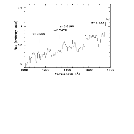
Fig. 9.: Portion of the long slit spectrum at low resolution. Ticks show the position of Lyman limits for some of the detected metal systems.

4.2 The associated systems

The abundances of the associated system have been determined in few cases and in all of them high ionization with high metal content has been derived (Møller et al. 1993; Wampler et al. 1993; Savaglio et al. 1994; Petitjean et al. 1994). In all these measurements different shapes have been assumed for the ionizing background, and this is presumably dominated by the flux of the QSO itself.

Indeed the distance of the cloud cannot be derived in a straightforward way because of the uncertainty in the measure of the systemic redshift and because of the importance of the cloud peculiar motions.

We found four associated systems, with a total of 11 components (Table 6). We estimate the metal abundances varying the intensity of the ionizing source using different values of the ionization parameter $U$. We assumed a simple power-law spectrum with spectral index $\alpha=1.5$ ($f_{\nu}\propto\nu^{-\alpha}$). Also a value $\alpha=0.72$ has been considered. The first value is a reasonable assumption for frequencies $\nu\geq 4\penalty 10000\kern 3.0ptRyd$ ($\lambda\leq 228$ Å), relevant for the considered ions, to keep the flux of the object at low values at X–ray frequencies. The second value is that used for the proximity effect and is more appropriate for $\nu\leq 1\penalty 10000\kern 3.0ptRyd$ ($\lambda\geq 912$ Å).

As for the intervening systems, all the absorption lines in every metal component are assumed to be originated in a single–phase gas cloud, with a uniform density and ionization state. The model results are shown in Fig.10 for five of the 11 measured components where the presence of silicon and/or nitrogen provides some constraints to the models.

For the strongest system at $z\sim 4.13$ the metal content of the third and fourth component is omitted because the relevant HI column densities are particularly uncertain due to the saturated and blended profile of the Ly$\alpha$lines. The Ly$\beta$lines fall in the blue wing of the damped Ly$\alpha$line at $z_{abs}$= 3.39, making the line fitting more complicated. The total HI column density is $\log N_{HI}\simeq 16.2$. From our grism spectrum we estimate an upper limit to the HI optical depth at 912 Å(Fig.9), corresponding to a total HI column density $\log N_{HI}\ \raise-2.0pt\hbox{\hbox to0.0pt{\hbox{$\sim$}\hss}\raise 5.0pt\hbox{$<$}\ }16$, consistent with the value found from our best fit. The OVI column densities reported in Table 6 are probably upper limits because of the confusion with the Ly$\alpha$forest and with the blue wing of the damped Ly$\alpha$line at $z_{abs}$= 3.39. For the three components considered in this analysis, results from the fit give ratios of the HI to OVI of $\log(N_{HI}/N_{OVI})\simeq-1.8,-3.9,-3.5$ respectively, suggesting the OVI contamination.

Concerning the other three systems at lower redshifts, only the first component of the system at $z\simeq 4.06$ shows SiIII and SiIV together with CIV. The SiIV line is observed also in the system at $z=4.1010$. For the system at $z=4.126$ we only give for the first component an upper limit to the SiIV abundance and a tentative SiIII identification in the Ly$\alpha$forest.

In Fig.10 we show CLOUDY results for the selected components of the associated systems. We report the metal abundances ([C/H]) and the relative abundance of nitrogen and silicon respect to carbon as a function of the ionization parameter $U$. The adopted gas density is $\log n_{H}=-2$ and the quasar spectral index is $\alpha=1.5$.

Fig. 10.: Metal content as function of the ionization parameter for five associated systems. We assume $\log n_{H}=-2$ and $\alpha=1.5$. Errors bars for [C/H] due to the errors on the column densities of HI and CIV are of about $0.2\penalty 10000\kern 3.0ptdex$, $0.06\penalty 10000\kern 3.0ptdex$, $0.3\penalty 10000\kern 3.0ptdex$, $1\penalty 10000\kern 3.0ptdex$ and $0.3\penalty 10000\kern 3.0ptdex$ for the five systems from the left to the right of the figure. Error bars for relative abundances of [C/Si] and [N/C] are typically of $0.1\penalty 10000\kern 3.0ptdex$.

Constraints to the model can be derived from the upper limits on CIII and from the detection of silicon. The upper limit to the column density of CIII gives a lower limit to the ionization parameter and an upper limit to the metallicity. The only exception is the $z=4.0606$ system for which we can only say that [C/Si] $>-1$ gives [C/H] $>-0.7$ and that the observed CIV can be reproduced only for $\log U>-2.4$

For the system at $z=4.1010$ the limits are $\log U>-2.3$ and [C/H] $<-0.3$. If we require a relative silicon abundance lower than 1 $dex$, the metallicity is [C/H] $\simeq-1$ and $\log U<-1.9$.

In the system at $z=4.1298$, the non detection of CIII implies $\log U>-1.9$ and consequently [C/H] $<-1.3$. The nitrogen relative abundance remains close to that solar.

In the system at $z=4.1311$, the upper limit to the CIII column density gives $\log U>-2.1$ and [C/H] $<-0.9$. The relative silicon abundance is lower than 1 $dex$ if [C/H] $>-1.5$. For $-1.5<$ [C/H] $<-0.9$, the relative nitrogen abundance is $-0.4<$ [N/C] $<-0.2$. In the last component, at $z=4.1342$, $\log U>-2.1$ and consequently [C/H] $<-0.3$. From the relative silicon abundance we derive [C/H] $>-0.9$. In this range of metallicity, the nitrogen abundance is $-0.3<$ [N/H] $<0.0$.

As for the intervening systems, errors on the HI column densities are much larger than for metal lines and relative metal abundances do not change rescaling the HI column density according to the upper and lower limit given by the errors, while the metallicity do.

From the analysis with $\alpha=1.5$, we conclude that in the detected metal systems the metallicity is undersolar, although values lower than [C/H] $\sim-1$ are unlikely. This value is about one order of magnitude higher than that found in intervening systems at about the same redshift. A silicon overabundance seems favoured, while the nitrogen abundance tends to be undersolar.

For $\alpha=0.72$, the values of [C/H] are higher with respect to the previous analysis, up to 0.2 $dex$ for the considered lower limit in the $\log U$ and of the order of 0.6 $dex$ for the upper limit of $\log U$. The [N/C] values are slightly lower, while the Silicon overabundance results much higher, being almost in all cases higher by 1 $dex$.

Savaglio et al. (1994) reported slightly higher values for the metallicity of the same associated systems. The greater wavelength coverage, the better $s/n$ of the present data and the new line fitting procedure adopted, allow a more accurate estimates of the line parameters. Moreover it was possible to detect new absorption lines and to infer more stringent upper limits to non–detected lines. In particular new upper limits on CIII absorptions have been used to derive upper limits on the metallicity. In this work we also used a more accurate photoionized code and we excluded the possibility of having silicon overabundances higher by 1 $dex$, lowering the upper limit to the metallicity. Finally, we have focused our attention on those systems for which we have reliable information only.

Metallicities derived for associated systems in $z_{em}=2-3$ quasars show nearly solar values and in some cases even higher than solar (Wampler et al. 1993; Petitjean et al. 1994; Møller et al. 1994). The lower metallicities derived for some systems at $z\simeq 4$ might be indicative of an evolution with redshift of the chemical abundances in the associated systems, which however needs confirmation with a larger sample of high quality data.

5 Summary

We have presented a list of absorption lines observed in the spectrum of the quasar Q$0000-2619$ ($z_{em}=4.126$) with a resolution of 13 kms^-1and a signal–to–noise ratio of $15-60$ per resolution element. The main results of the statistical analysis can be summarized as follows:

• The mode of the Doppler distribution for the Ly$\alpha$lines is $\simeq 25$ kms^-1with a dispersion of 7 kms^-1. The fraction of line with $10<b<20$ kms^-1is 17%. The Doppler values derived from uncontaminated Ly$\beta$lines are smaller than those obtained from the corresponding Ly$\alpha$, suggesting the contribution of non saturated, non resolved components in the Ly$\alpha$profiles.

• On the basis of the proximity effect in this spectrum the integrated UV background is estimated to be $J\sim 7\times 10^{-22}$ erg s^-1 cm^-2 Hz^-1 sr^-1, although only values of $J_{-22}<4$ and $J_{-22}>18$ are excluded at more than $2\sigma$ level. This value is consistent with previous estimates obtained at a lower $z$, implying no appreciable redshift evolution of the UVB up to $z=4$, in agreement with the absence of any Gunn-Peterson effect up to $z=5$.

• The analysis of the intervening metal line systems has revealed in particular the presence of three optically thin systems with $\log N_{HI}\sim 15$ showing associated CIV and SiIV absorptions. [Si/C] ratios lower than 10 times the solar value can be obtained only assuming a large jump in the spectrum of the ionizing UV background beyond the HeII edge ($J_{912}/J_{228}\ \raise-2.0pt\hbox{\hbox to0.0pt{\hbox{$\sim$}\hss}\raise 5.0pt\hbox{$>$}\ }1000$). This result, if confirmed in other spectra at the same redshift, is suggestive of a possible increase of the stellar ionizing emissivity over the declining quasar one for $z>3$.

• The analysis of the associated metal line systems suggests abundances generally below solar with typical values in the range $0<$ [C/H]$<-1$. The derived values are lower than those estimated for associated systems found in lower $z$ quasars.

Acknowledgements.

It is a pleasure to thank M.Limongi and G.Marconi for useful remarks on an early version of the paper. S.S. acknowledges the kind hospitality at the Osservatorio Astronomico di Roma where most of this work was done.

References

- 1986 Bahcall J.N., et al., 1996, ApJ, 457, 19.
- 1986 Bajtlik, S., Duncan, R. C., Ostriker, J. P. 1988, ApJ, 327, 570.
- 1986 Bergeron J., Boissé P., 1991, A&A, 243, 344.
- 1986 Bergeron J., Cristiani S., Shaver, P.A., 1992, A&A, 257, 417.
- 1986 Carswell R.F., 1995, Proceedings of the ESO Workshop on Quasars Absorption Lines, ed.G.Meylan, p313.
- 1986 Charlton J.C., 1995, Proceedings of the ESO Workshop on Quasars Absorption Lines, ed.G.Meylan, p405.
- 1986 Chernomordik V.V., 1995, ApJ, 440, 431.
- 1986 Cowie L.L., Songaila A., Kim T.-S., Hu E. M., 1995, AJ, 109, 1522.
- 1986 Cristiani S., D’Odorico S., D’Odorico V.,Fontana A., Giallongo E., Savaglio S., 1996, MNRAS, submitted.
- 1986 Cristiani, D’Odorico, S., Fontana, A, Giallongo, E., Savaglio, S., 1995, MNRAS, 273, 1016.
- 1986 Davidsen A.F., Kriss G.A., Zheng W., 1996, Nat, 380, 47.
- 1986 D’Odorico, S. 1990, ESO The Messenger, 61, 51.
- 1986 Espey, B. R. 1993, ApJL, 411, 59.
- 1986 Ferland G.J., 1991, OSU Astronomy Dept.Internal Rept., 91-01
- 1986 Fernández–Soto A., Lanzetta K.M., Barcons X., Carswell R.F., Webb J.K., Yahil A., 1996, ApJ, 460, L85.
- 1986 Ferrara A., Giallongo E., 1996, MNRAS, in press.
- 1986 Fontana A., Ballester P., 1995, ESO The Messenger, 80, 37.
- 1986 Giallongo E., Cristiani, S., D’Odorico S., Fontana A., Savaglio S., 1996, ApJ, in press.
- 1986 Giallongo, E., Cristiani, S., Fontana, A., Trevese, D. 1993, ApJ, 416, 137.
- 1986 Giallongo, E., D’Odorico, S., Fontana, A., McMahon, R. G., Savaglio, S., Cristiani, S., Molaro, P., Trevese, D. 1994, ApJL, 425, L1.
- 1986 Giallongo E., Petitjean P., 1994, ApJ, 426, L61.
- 1986 Haardt F., Madau P., 1996, ApJ, 461, 20.
- 1986 Hernquist L., Katz N., Weinberg D..H., Miralda–Escudé J., 1996, ApJ, 457, L51.
- 1986 Hu E.M., Kim T.-S., Cowie L.L., Songaila A., Rauch M., 1995, AJ, 110, 1526.
- 1986 Jakobsen P., Boksenberg A., Deharveng J.M., Greenfield P., Jedrzejewski R., Paresce F., 1994, Nat, 370, 35.
- 1986 Lanzetta, K.M., Bowen, D.V., Tytler, D., Webb, J.K., 1995, ApJ, 442, 538.
- 1986 Lu L., Sargent W.L.W., Barlow T.A., 1996, Contribution to ”Cosmic Abundances”, the proceedings of the 6th Annual October Astrophysical Conference in Maryland, in press.
- 1986 Madau P., 1992, ApJ, 389, L1.
- 1986 Miralda–Escudé J., Ostriker J.P., 1990, ApJ, 350, 1.
- 1986 Miralda–Escudé J., Cen R., Ostriker J.P., Rauch M., 1996, ApJ, submitted.
- 1986 Molaro, P., D’Odorico, S., Fontana, A., Savaglio, S., Vladilo, G., 1995, A&A, 308, 1.
- 1986 Møller P., Jakobsen P., Perryman M.A.C., 1993, A&A, 287, 719.
- 1986 Pei Y.C., 1995, ApJ, 438, 623.
- 1986 Petitjean P., Bergeron J., 1994, A&A, 283, 759.
- 1986 Petitjean P., Rauch M., Carswell R.F., 1994, A&A, 291, 29.
- 1986 Rauch M., Carswell R.F., Webb J.K., Weymann R.J., 1993, MNRAS, 260, 589.
- 1986 Savaglio S., D’Odorico S., Møller P., 1994, A&A, 281, 331.
- 1986 Schneider, D.P., Schmidt, M., Gunn, J.E., 1989, AJ, 98, 1507.
- 1986 Songaila A., Hu E.M., Cowie L.L., 1995, Nat, 375, 124.
- 1986 Steidel C.C., Dickinson M., Persson S.E., 1994, ApJ, 437, L75.
- 1986 Stone, R. P. S. 1977, Ap. J., 218, 767.
- 1986 Stone, R. P. S., Baldwin, J. A. 1983, MNRAS, 204, 347.
- 1986 Stone, R. P. S., Baldwin, J. A. 1984, MNRAS, 206, 241.
- 1986 Timmes F.X., Woosley S.E., Weaver T.A., 1995, ApJS, 98, 617.
- 1986 Tytler D., Fan X.-M., Burles S., Cottrell L., Davis C., Kirkman D., Zuo L., 1995, Proceedings of the ESO Workshop on Quasars Absoon Lines, ed.G.Meylan, p289.
- 1986 Wheeler J.C., Sneden C., Truran J.W., 1989, ARA&A, Vol.27, ed.G.Burbidge (Palo Alto: Annual Reviews), 279.
- 1986 Walsh J.R., 1992, HST and New Oke Spectrophotometric Standard Stars–Flux Tables and Finding Charts.
- 1986 Wampler E.J., Bergeron J., Petitjean P., 1993, A&A, 273, 15.
- 1986 Webb J.K., Parnell H.C., Carswell R.F., McMahon R.G., Irwin M.J., Hazard C., Ferlet R., Vidal–Madjar A. 1988, The ESO Messenger, 51, 15.
- 1986 Williger G.M., Baldwin J.A., Carswell R.F., Cooke A.J., Hazard C., Irwin M.J., McMahon R.G., Storrie–Lombardi L., 1994, ApJ, 428, 574.