GRAVITATIONAL MICROLENSING IN THE LOCAL GROUP

Abstract

The status of searches for gravitational microlensing events of the stars in our galaxy and in other galaxies of the Local Group, the interpretation of the results, some theory, and prospects for the future are reviewed. The searches have already unveiled $\sim 100$ events, at least two of them caused by binaries, and have already proven to be useful for studies of the Galactic structure. The events detected so far are probably attributable to the effects of ordinary stars, and possibly to sub-stellar brown dwarfs; however a firm conclusion cannot be reached yet because the analysis published to date is based on a total of only 16 events. The current searches, soon to be upgraded, will probably allow determination of the mass function of stars and brown dwarfs in the next few years; these efforts will also provide good statistical information about binary systems, in particular their mass ratios. They may also reveal the nature of dark matter and allow us to detect planets and planetary mass objects.

1 Introduction

The topic of gravitational lensing has a long history, as described for example in the first book entirely devoted to the subject (Schneider et al. 1992). The first known theoretical calculation of a light ray bending by massive objects was published by Soldner (1801), who used Newtonian mechanics, and determined that the deflection angle at the solar limb should be $0.^{\prime\prime}84$, half the value calculated with the general theory of relativity (Einstein 1911, 1916). The first observational detection of this effect came soon afterwards (Dyson et al. 1920). Zwicky (1937) pointed out that distant galaxies may act as gravitational lenses. Almost all essential formulae used today to analyze gravitational lensing were derived by Refsdal (1964). The first case of a double image created by gravitational lensing of a distant source, the quasar 0957+561, was discovered by Walsh et al. (1979). Arc–like images of extended sources, the galaxies, were first reliably reported by Lynds & Petrosian (1989). In these three cases the sun, a galaxy, and a cluster of galaxies, were acting as gravitational lenses. There are many recent review articles (Blandford & Narayan 1992, Refsdal & Surdej 1994, Roulet & Mollerach 1996) and international conferences (Moran et al. 1989, Mellier et al. 1990, Kayser et al. 1992, Surdej et al. 1993, Kochanek & Hewitt 1996) on the subject of gravitational lensing. A review of gravitational microlensing experiments has been published by Ansari (1995).

The effect of double imaging of a distant source by a point mass located close to the line of sight, and acting as a gravitational lens, has been proposed many times over. Chang and Refsdal (1979) and Gott (1981) noted that even though a point mass in a halo of a distant galaxy would create an unresolvable double image of a background quasar, the time variation of the combined brightness of the two images could be observed. This way the effect of non-luminous matter in a form of brown dwarfs or Jupiters could be detected. The term “microlensing” was proposed by Paczyński (1986a) to describe gravitational lensing which can be detected by measuring the intensity variation of a macro–image made of any number of unresolved micro–images.

Paczyński (1986b) suggested that a massive search of light variability among millions of stars in the Large Magellanic Cloud could be used to detect dark matter in the galactic halo. Luckily, the technology needed for such a search became available soon afterwards, and the 1986 paper is credited with triggering the current microlensing searches: EROS (Aubourg et al. 1993), MACHO (Alcock et al. 1993), OGLE (Udalski 1992), and DUO (Alard 1996b, Alard et al. 1995a). Griest (1991) proposed that objects responsible for gravitational microlensing be called massive astrophysical compact halo objects (MACHO). The name became very popular and it is commonly used to refer to all objects responsible for the observed microlensing events, no matter where they are located and what their mass may be.

It is not possible to discuss all theoretical and observational papers related to microlensing in the Local Group within the modest volume of this article. The selection of references at the end of this review is limited, and I apologize for all omissions, and for the way I made the selection. Let us hope that somebody will write a more careful historical review before too long. Fortunately, there is a bibliography of over one thousand papers that are related to gravitational lensing, and it is available electronically. This bibliography has been compiled, and it is continuously updated, by J. Surdej and by A. Pospieszalska. It can be found on the World Wide Web at:

http://www.stsci.edu/ftp/stsci/library/grav_ lens/grav_ lens.html

The MACHO and the OGLE collaborations provide up-to-date information about their findings and a complete bibliography of their work on the World Wide Web and by anonymous ftp. The photometry of OGLE microlensing events, their finding charts, as well as a regularly updated OGLE status report, including more information about the “early warning system”, can be found over Internet from the host:

sirius.astrouw.edu.pl      (148.81.8.1) ,

using “anonymous ftp” service (directory “ogle”, files “README”, “ogle.status”, “early.warning”). The file “ogle.status” contains the latest news and references to all OGLE related papers, and PostScript files of some publications. These OGLE results are also available over World Wide Web at:

http://www.astrouw.edu.pl          (Europe).

A duplicate of this information is available at

http://www.astro.princeton.edu/~ogle/          (North America).

A complete information about MACHO results is available at:

http://wwwmacho.mcmaster.ca/          (North America)

with a duplicate at

http://wwwmacho.anu.edu.au/          (Australia).

The information about MACHO alerts is to be found at:

http://darkstar.astro.washington.edu/

No doubt other groups will provide similar information before too long. The main weakness of this electronic information distribution is the frequent change of address and mode of access. I shall do my best to keep a guide to this information as part of the OGLE home page on the WWW.

In the following section a simple model of lensing by an isolated point mass is presented – this is all theory one needs to understand most individual microlensing events. The third section presents a model for the space distribution and kinematics of lensing objects in order to provide some insight into problems in relating the observed time scales of microlensing events to the masses of lensing objects. The fourth section provides a glimpse of diversity of light curves due to lensing by double objects, like binary stars or planetary systems. Some of the special effects which make microlensing more complicated than originally envisioned are described in the fifth section. The most essential information about the current searches for microlensing events, and some of the results as well as problems with some results, are presented in section six. The last section is a rather personal outline of the prospects for the future of microlensing searches.

2 Single point mass lens

Let us consider a single point mass $M$ (a deflector) at a distance $D_{d}$ from the observer, and a point source $S$ at a distance $D_{s}$ from the observer, as in Figure 1. Let there be two planes perpendicular to the line of sight, at the deflector and the source distances, respectively. The deflector has angular coordinates $(x_{m},y_{m})$ in the sky, as seen by the observer. This projects into points $M$ and $M_{s}$ in the two planes, with the corresponding linear coordinates:

Figure 1: The geometry of gravitational lensing is shown. The observer, the lensing mass, and the source are located at the points $O$, $M$, and $S$, respectively. The light rays are deflected near the lensing mass by the angle $\alpha$, and the image of the source appears to be located at the point $I$, not at $S$. The distances from the observer to the lens (deflector) and to the source are indicated as $D_{d}$ and $D_{s}$, respectively.

Figure 2: The geometry of gravitational lensing is shown. The lensing mass, the small circular source, and the two images are marked with $M$, $S$, $I_{1}$, and $I_{2}$, respectively. Of course, in the presence of mass $M$ the source is not seen at $S$ but only at $I_{1}$ and $I_{2}$. The Einstein ring is shown as a dashed circle. A typical radius of the circle is $\sim 1$ milli arc second for microlensing by stars in our galaxy.

$$X_{M}=x_{m}D_{d},\hskip 28.45274ptY_{M}=y_{m}D_{d},$$

$$X_{M,s}=x_{m}D_{s},\hskip 28.45274ptY_{M,s}=y_{m}D_{s}.$$

Let the observer, located at point $O$, look at the sky in the direction with angular coordinates $(x,y)$. The line of sight intersects the deflector plane at point $A$ with coordinates:

$$X_{A}=xD_{d},\hskip 28.45274ptY_{A}=yD_{d}.$$

If there was no deflection of light by the massive object then the line of sight would intersect the source plane at point $I$ with coordinates:

$$X_{I}=xD_{s},\hskip 28.45274ptY_{I}=yD_{s}.$$

In fact the light ray passes the deflector at a distance

$$R=\left[\left(X_{A}-X_{M}\right)^{2}+\left(Y_{A}-Y_{M}\right)^{2}\right]^{1/2}.$$

As a consequence of general relativity the light ray is deflected by the angle

$$\alpha={4GM\over Rc^{2}},$$

with the two components:

$$\alpha_{x}=\alpha{X_{A}-X_{M}\over R},\hskip 28.45274pt\alpha_{y}=\alpha{Y_{A}-Y_{M}\over R}.$$

The deflected light ray intersects the source plane at the point $S$ with the coordinates:

$$X_{S}=X_{I}-\alpha_{x}(D_{s}-D_{d}),\hskip 28.45274ptX_{S}=Y_{I}-\alpha_{y}(D_{s}-D_{d}),$$

Passing through three points: $O$, $A$ , and $S$, the light ray defines a plane. The lensing mass $M$, and the point $I$ are also located in the same plane, as shown in Fig. 1. If there was no effect of the mass $M$ on the light rays then the source of light would be seen at the point $S$, at the angular distance $R_{s}/D_{d}$ from the point $M$. However, as the light rays are deflected by $M$ the image of the source appears not at S but at the point $I$, at the angular distance $R/D_{d}$ from the point $M$. It is clear that the distance $(R+R_{s})$ in the deflector plane is proportional to the distance between $I$ and $S$ in the source plane, and the latter can be calculated with the eqs. (6). Combining this with the eqs. (5) and (4) we obtain:

$$R+R_{s}=\left[\left(X_{S}-X_{I}\right)^{2}+\left(Y_{S}-Y_{I}\right)^{2}\right]^{1/2}{D_{d}\over D_{s}}=\alpha\left(D_{s}-D_{d}\right){D_{d}\over D_{s}}={4GM\over Rc^{2}}{\left(D_{s}-D_{d}\right)D_{d}\over D_{s}}.$$

This equation may be written as

$${R_{\rm s}\over R_{\rm E}}=-{R\over R_{\rm E}}+{R_{\rm E}\over R},\hskip 28.45274ptR^{2}+R_{\rm s}R-R_{\rm E}^{2}=0,$$

where

$$R_{E}^{2}\equiv 2R_{g}D,\hskip 28.45274ptR_{g}\equiv{2GM\over c^{2}},\hskip 28.45274ptD\equiv{\left(D_{s}-D_{d}\right)D_{d}\over D_{s}},$$

and $R_{E}$, $R_{g}$, and $D$ are called the linear Einstein ring radius of the lens, the gravitational radius of the mass $M$, and the effective lens distance, respectively.

The equation (8a) has two solutions:

$$R_{+,-}=0.5\left[R_{s}\pm\left(R_{s}^{2}+4R_{E}^{2}\right)^{1/2}\right].$$

These two solutions correspond to the two images of the same source, located on the opposite sides of the point $M$, at the angular distances of $R_{+}/D_{d}$ and $R_{-}/D_{d}$, respectively. The appearance of a small circular source (in the absence of lensing) and its two distorted two images in a telescope with very high resolving power is shown in Fig. 2. As any lensing conserves surface brightness (cf. Schneider et al. 1992, section 5.2), the ratio of the image to source intensity is given by the ratio of their areas. With the geometry shown in Fig. 2 this ratio can be calculated as

$$A_{+,-}=\left|{R_{+,-}\over R_{s}}~{}{dR_{+,-}\over dR_{s}}\right|={u^{2}+2\over 2u\left(u^{2}+4\right)^{1/2}}\pm 0.5,\hskip 28.45274ptu\equiv{R_{s}\over R_{E}},$$

assuming that the source is very small. The quantity $A$ is called magnification or amplification. The term magnification will be used throughout this paper, as it better describes the lensing process. The total magnification of the two images can be calculated as

$$A=A_{+}+A_{-}={u^{2}+2\over u\left(u^{2}+4\right)^{1/2}}.$$

It is interesting to note that this is always larger than unity. It is also interesting that the difference in the magnification of the two images is constant:

$$A_{+}-A_{-}=1.$$

Let us consider a typical galactic case, with a lens of $\sim 1~{}M_{\odot}$ mass at a distance of a few kiloparsecs, and the source at a larger distance. The angular Einstein ring radius, $r_{{}_{E}}$, can be calculated with the eqs. (8b) to be

$$r_{{}_{E}}\equiv{R_{E}\over D_{d}}=\left[\left({4GM\over c^{2}}\right)~{}\left({D_{s}-D_{d}\over D_{s}D_{d}}\right)\right]^{1/2}=$$

$$=0.902~{}mas~{}\left({M\over M_{\odot}}\right)^{1/2}\left({10~{}kpc\over D_{d}}\right)^{1/2}\left(1-{D_{d}\over D_{s}}\right)^{1/2}.$$

With the image separation $\sim 2r_{{}_{E}}$, i.e. of the order of a milliarcsecond (mas), we can only see the combined light intensity, rather than two separate images because of the limited resolution of optical telescopes. Fortunately, all objects in the galaxy move, and we may expect a relative proper motion to be

$$\dot{r}={V\over D_{d}}=4.22~{}mas~{}yr^{-1}~{}\left({V\over 200~{}km~{}s^{-1}}\right)\left({10~{}kpc\over D_{d}}\right),$$

Figure 3: The geometry of gravitational lensing is shown. The lensing mass is indicated with a dot at the center of the Einstein ring, which is marked with a dashed line. The source positions are shown with a series of small open circles. The locations and the shapes of the two images are shown with a series of dark ellipses. At any instant the two images, the source and the lens are all on a single line, as shown in the figure for one particular instant.

where $V$ is the relative transverse velocity of the lens with respect to the source. Combining the last two equations we can calculate the characteristic time scale for a microlensing phenomenon as the time it takes the source to move with respect to the lens by one Einstein ring radius:

$$t_{0}\equiv{r_{{}_{E}}\over\dot{r}}=0.214~{}yr~{}\left({M\over M_{\odot}}\right)^{1/2}\left({D_{d}\over 10~{}kpc}\right)^{1/2}\left(1-{D_{d}\over D_{s}}\right)^{1/2}\left({200~{}km~{}s^{-1}\over V}\right).$$

This definition is almost universally accepted, with one major exception: the MACHO collaboration multiplies the value of $t_{0}$ as given with the eq. (15) by a factor 2.

Figure 4: The geometry of gravitational lensing is shown. The lensing mass $M$ is located at the center of the Einstein ring, which is marked with a dashed line. The twelve horizontal lines represent relative trajectories of the source, labeled with the value of dimensionless impact parameter $p$.

Figure 5: The variation of the magnification due to a point gravitational lensing is shown in stellar magnitudes as a function of time. The unit $t_{0}$ is defined as the time it takes the source to move a distance equal to the Einstein ring radius, $r_{E}$. The six light curves correspond to the six values of the dimensionless impact parameter: $p=0.1,~{}0.3,~{}0.5,~{}0.7,~{}0.9,~{}1.1$.

While the lens moves with respect to the source the two images change their position and brightness, as shown in Fig. 3. When the source is close to the lens the images are highly elongated and their proper motion is much higher than that of the source. Note, that for each source position the two images, the source and the lens are all located on a straight line which rotates around the lens. Unfortunately, none of this geometry can be observed directly for the stellar mass lenses, as the angular scale is of the order of a milli arcsecond. The total light variations can be observed, and the light curve can be calculated with the eq. (11). The variable $u$ can be determined as

$$u=\left[p^{2}+\left({t-t_{max}\over t_{0}}\right)^{2}\right]^{1/2},$$

where $p$ is the dimensionless impact parameter: the smallest angular distance between the source and the lens measured in units of Einstein ring radius, and $t_{max}$ is the time of the maximum magnification by the lens. The geometry of lensing for six values of impact parameter, and the corresponding time variability expressed in stellar magnitudes: $\Delta m\equiv 2.5\log A$, are shown in Figs. 4 and 5.

It is customary to define the cross section for gravitational microlensing to be equal to the area of the Einstein circle. The combined magnification of the two images of a source located within that circle is larger than

$$A\geq{3\over 5^{1/2}}=1.3416,\hskip 28.45274pt\Delta m\geq 0.3191~{}mag,\hskip 28.45274pt(u\leq 1),$$

(cf. eq. 11) i.e. it is easy to detect such intensity variation with a reasonably accurate photometry.

Let there be many lensing objects in the sky. The fraction of solid angle covered with their Einstein rings is called the optical depth to gravitational microlensing. Let all lensing objects have identical masses $M$. In a thin slab at a distance $D_{d}$ and a thickness $\Delta D_{d}$, there is, on average, one lens per surface area $\pi R_{M}^{2}=M/(\rho\Delta D_{d})$, where $\rho$ is the average mass density due to lenses in the volume $\pi R_{\rm M}^{2}\Delta D_{\rm d}$. Each lens has a cross section $\pi R_{E}^{2}$, with the Einstein ring radius $R_{E}$ given with the eqs. (8b). The slab contribution to the optical depth is given as

$$\Delta\tau={\pi R_{E}^{2}\over\pi R_{M}^{2}}=\left[{4\pi G\rho\over c^{2}}~{}{D_{d}\left(D_{s}-D_{d}\right)\over D_{s}}\right]\Delta D_{d}.$$

The total optical depth due to all lenses between the source and the observer can be calculated as

$$\tau=\int_{0}^{D_{s}}{4\pi G\rho\over c^{2}}~{}{D_{d}\left(D_{s}-D_{d}\right)\over D_{s}}~{}dD_{d}={4\pi G\over c^{2}}D_{s}^{2}\int_{0}^{1}\rho(x)~{}x(1-x)~{}dx,$$

where $x\equiv{D_{d}/D_{s}}$. Note that the optical depth $\tau$ depends on the total mass in all lenses, but it is independent of the masses of individual lenses, $M$. If the density of matter is constant then we have

$$\tau={2\pi\over 3}~{}{G\rho\over c^{2}}~{}D_{s}^{2}.$$

If the system of lenses is self-gravitating, then a crude but very simple estimate of the optical depth can be made. Let us suppose that the distance to the source $D_{s}$ is approximately equal to the size of of the whole system, a galaxy of lenses. The virial theorem provides a relation between the velocity dispersion $V^{2}$, the density $\rho$, and the size $D_{s}$:

$${GM_{tot}\over D_{s}}\approx{G\rho D_{s}^{3}\over D_{s}}\approx V^{2}.$$

Combining eqs. (20) and (21) we obtain

$$\tau\approx{V^{2}\over c^{2}}.$$

A more accurate estimate of the optical depth can be obtained by evaluating the integral in eq. (19) for any distribution of mass density along the line of sight.

3 The event rate and the lens masses

We now proceed to the estimate of the number of microlensing events $N$ that may be expected if $n$ sources are monitored over a time interval $\Delta t$. We consider only those microlensing events which have peak magnification in excess of $3/\sqrt{5}$, i.e. their dimensionless impact parameters are smaller than unity (cf. Figures 4 and 5). We begin with the simplest case: all lensing objects have the same mass $M$, and all have the same 3-dimensional velocity $V$. We also assume that the velocity vectors have a random but isotropic distribution, the source located at the distance $D_{s}$ is stationary, and the number density of lensing objects is statistically uniform between the observer and the source.

The time scale of a microlensing event is given as

$$t_{0}={r_{{}_{E}}\over\dot{r}}={R_{E}\over V_{t}}={R_{E}\over V\sin i},$$

(cf. eq. 15) where $i$ is the angle between the velocity vector and the line of sight, and $V_{t}=V\sin i$ is the transverse velocity of the lens. If all events had identical time scales, then the number of microlensing events expected in a time interval $\Delta t$ would be given as

$$N={2\over\pi}~{}n\tau~{}{\Delta t\over t_{0}},$$

for $t_{0}=const$, where $2/\pi$ is the ratio of Einstein ring diameter to its area, in dimensionless units, and $\tau$ is the optical depth.

In fact there is a broad distribution of event time scales as lenses (all with the same mass $M$ and the same space velocity $V$) have transverse velocities in the range $0\leq V_{t}\leq V$, and distances in the range $0\leq D_{d}\leq D_{s}$. Straightforward but tedious algebra leads to the equation

$$N={3\pi\over 16}~{}n\tau~{}{\Delta t\over t_{m}}=\int_{0}^{\infty}N^{\prime}(t_{0})~{}dt_{0},$$

where

$$t_{m}\equiv\left({R_{E}\over V}\right)_{D_{d}=0.5D_{s}}=\left({GMD_{s}\over c^{2}}\right)^{1/2}{1\over V},$$

is the time scale for a microlensing event due to a lens located half way between the source and the observer, and moving with the transverse velocity $V$. A detailed analysis is given by Mao & Paczyński (1996).

The probability distribution of event time scales is very broad. It can be shown to have power-law tails for very short and for very long time scales:

$$P(t_{0}\leq t^{\prime})={128\over 45\pi^{2}}\left(t^{\prime}\over t_{m}\right)^{3},\hskip 28.45274pt{\rm for}\hskip 14.22636ptt^{\prime}\ll t_{m},$$

$$P(t_{0}\geq t^{\prime})={128\over 45\pi^{2}}\left(t_{m}\over t^{\prime}\right)^{3},\hskip 28.45274pt{\rm for}\hskip 14.22636ptt^{\prime}\gg t_{m}.$$

Note that the power law tails in the distribution of event time scales are generic to almost all lens distributions ever proposed. The very short events are due to lenses which are either very close to the source or very close to the observer, while the very long events are caused by the lenses which move almost along the line of sight. Also note that only the first two moments of the distribution are finite; the third and higher moments diverge. Therefore, it is convenient to use a logarithmic probability distribution defined as

$$p(\log t_{0})~{}d\log t_{0}=\left({\ln 10\over N}\right)~{}t_{0}~{}N^{\prime}(t_{0})~{}d\log t_{0},$$

as all moments of this distribution are finite.

De Rújula et al. (1991) proposed to use the moment analysis to deduce the distribution of lens masses. We shall carry on such an analysis, but first we have to make our model more realistic. As most astrophysical objects have a broad range of velocities, we adopt a 3-dimensional gaussian distribution:

$$p(V)~{}{dV\over V_{rms}}=3\left(6\over\pi\right)^{1/2}~{}\exp\left(-{3V^{2}\over 2V_{rms}^{2}}\right)~{}{V^{2}~{}\over V_{rms}^{2}}~{}{dV\over V_{rms}},\hskip 28.45274pt{\rm for}\hskip 14.22636pt0\leq V<\infty.$$

where the 3–dimensional rms velocity $V_{rms}$ is defined as

$$V_{rms}^{2}\equiv\int_{0}^{\infty}V^{2}p(V)~{}{dV\over V_{rms}},$$

We also adopt a general power law distribution of the number of lensing masses:

$$n(M)~{}dM\sim M^{\alpha}~{}dM,\hskip 28.45274pt{\rm for}\hskip 14.22636ptM_{min}\leq M\leq M_{max},$$

or, in a logarithmic form:

$$n(\log M)~{}d\log M=\left[{(\alpha+1)\ln 10\over M_{max}^{\alpha+1}-M_{min}^{\alpha+1}}\right]~{}M^{\alpha+1}~{}d\log M,\hskip 28.45274pt{\rm for}\hskip 14.22636pt\alpha\neq-1,$$

$$n(\log M)~{}d\log M=\left[{\ln 10\over\ln\left(M_{max}/M_{min}\right)}\right]~{}d\log M,\hskip 28.45274pt{\rm for}\hskip 14.22636pt\alpha=-1.$$

The case $\alpha=-2$ corresponds to equal total mass per decade of lens masses, i.e. each decade has the same contribution to the optical depth. The case $\alpha=-1.5$ corresponds to equal rate of microlensing events per decade of lens masses. If the mass function is very broad, i.e. $M_{max}/M_{min}\gg 1$, then the distribution of event rate will be flat in this case, with equal number of events per logarithmic interval of $t_{0}$, with power law tails (cf. eqs. 27 and 28). If $\alpha=-1$ then there is equal number of lenses per logarithmic interval of their masses.

A characteristic mass scale for the lenses can be related to the first moment of the $t_{0}$ distribution:

$$M_{0}\equiv{c^{2}V_{rms}^{2}\over GD_{s}}~{}t_{0,av}^{2},\hskip 28.45274pt{\rm where}\hskip 14.22636pt\log t_{0,av}\equiv\langle\log t_{0}~{}\rangle,$$

(cf. eqs. 26, 30). The value of $M_{0}$ is indicative of the most common lens mass. However, for $\alpha\ll-1.5$ the mass spectrum is dominated by low mass objects, the event time scales have a small effective range, and the events are mostly due to lenses with $M\approx M_{min}$. In the opposite case, with $\alpha\gg-1.5$, the microlensing events are dominated by lenses with $M\approx M_{max}$.

For a given mass range the standard deviation of $\log t_{0}$ is the largest for $\alpha=-1.5$, and it can be estimated analytically. First, imagine that there is a unique relation between the lens mass $M$ and the event time scale $t_{0}$. The exponent $\alpha=-1.5$ implies a uniform distribution of event time scales in $\log t_{0}$ over the range $\log t_{min}\leq\log t_{0}\leq\log t_{max}$, with $\log~{}(t_{max}/t_{min})=0.5\log~{}(M_{max}/M_{min})=0.5\Delta\log M$. This distribution would have a standard deviation $\sigma_{\log t_{0}}=(\Delta\log M)^{2}/48$. However, there is no unique relation between the lens mass and the corresponding time scale $t_{0}$ in our model. Even if all lenses had the same mass the standard deviation would be $\sigma_{0}=0.268$, according to numerical calculations. Therefore, the following formula can be used to calculate the second moment:

$$\sigma_{\log t_{0}}=\left[\sigma_{0}^{2}+{(\Delta\log M)^{2}\over 48}\right]^{1/2},\hskip 14.22636pt\sigma_{0}=0.268,\hskip 28.45274pt{\rm for}\hskip 14.22636pt\alpha=-1.5.$$

There is another serious problem affecting the relation between the observed event time scales and the lens masses. In general we do not know which model should be adopted for the space distribution of lenses and for their kinematics. For the purpose of our exercise we adopted a uniform space density and a uniform velocity distribution, all the way from the source to the observer. Unfortunately, there is no consensus yet on the distribution and the kinematics of the dominant lensing component towards the galactic bulge and towards the LMC. To reach a consensus it will be necessary to determine observationally the variation of optical depth to microlensing with the galactic coordinates, and to use this information to determine the space distribution of the dominant lens population. Next, a model of the galactic gravitational potential will have to be used to estimate the kinematics of the dominant lens population. In order to have confidence that the observed distribution of event time scales is not truncated by instrumental effects the power law tails, like those given with the eqs. (27) and (28), will have to be well sampled. When all this work is done a relation between the distribution of event time scales and the distribution of lens masses will be sound.

4 Double lenses and planets

Let us consider now a large number of point mass lenses, all located at the same distance $D_{d}$, in front of a point source at $D_{s}$. Let a lens number “i” has a mass $M_{i}$ located at $(X_{i},Y_{i})$. A light ray crossing the deflector’s plane at $(X,Y)$ would pass at a distance $R_{i}$ from the lens “i”:

$$R_{i}=\left[\left(X-X_{i}\right)^{2}+\left(Y-Y_{i}\right)^{2}\right]^{1/2},$$

(cf. eq. 3). The contribution to the light ray deflection by the mass “i” is given by the angle

$$\alpha_{i}={4GM_{i}\over R_{i}c^{2}},$$

with the two components:

$$\alpha_{x,i}=\alpha_{i}~{}{X-X_{i}\over R_{i}},\hskip 28.45274pt\alpha_{y,i}=\alpha_{i}~{}{Y-Y_{i}\over R_{i}},$$

(cf. eqs. 4 and 5). As a result the combined deflection by all lensing masses the light ray will cross the source plane at $(X_{S},Y_{S})$:

$$X_{S}=X{D_{s}\over D_{d}}-\sum_{i}\alpha_{x,i}(D_{s}-D_{d}),\hskip 28.45274ptY_{S}=Y{D_{s}\over D_{d}}-\sum_{i}\alpha_{y,i}(D_{s}-D_{d}),$$

(cf. eq. 6). Note that $X,~{}Y,~{}X_{i},~{}Y_{i},$ and $R_{i}$ are all measured in the deflector plane, while $X_{s}$ and $Y_{s}$ are measured in the source plane.

Combining eqs. (38–40) we obtain

$$x_{s}=x-{(D_{s}-D_{d})\over D_{s}D_{d}}~{}\sum_{i}{4GM_{i}\over c^{2}}~{}{(x-x_{i})\over r_{i}^{2}},$$

$$y_{s}=y-{(D_{s}-D_{d})\over D_{s}D_{d}}~{}\sum_{i}{4GM_{i}\over c^{2}}~{}{(y-y_{i})\over r_{i}^{2}},$$

where the angles are defined as

$$x_{s}={X_{S}\over D_{s}},\hskip 14.22636pty_{s}={Y_{S}\over D_{s}},$$

and

$$x={X\over D_{d}},\hskip 14.22636pty={Y\over D_{d}},\hskip 14.22636ptx_{i}={X_{i}\over D_{d}},\hskip 14.22636pty_{i}={Y_{i}\over D_{d}},\hskip 14.22636ptr_{i}={R_{i}\over D_{d}}.$$

With dimensionless masses $m_{i}$ defined as

$$m_{i}={(D_{s}-D_{d})\over D_{s}D_{d}}~{}{4GM_{i}\over c^{2}},$$

the eqs. (41–42) may be written as

$$x_{s}=x-~{}\sum_{i}~{}{m_{i}(x-x_{i})\over r_{i}^{2}},$$

$$y_{s}=y-~{}\sum_{i}~{}{m_{i}(y-y_{i})\over r_{i}^{2}}.$$

All these are angles as seen by the observer.

The set of equations (46–47) can be used to find all images created by a planar lens system made of any number of point masses (cf. Witt 1993, and references therein). Here we shall restrict ourselves to a double lens case, as binary stars are known to be very common (Abt 1983, Mao & Paczyński 1991). A very thorough analysis of double star microlensing is provided by Schneider & Weiss (1986). A major new phenomenon not present in a single lens case is the formation of caustics caused by the lens astigmatism. When a source crosses a caustic a new pair of images forms or disappears. A point source placed at a caustic is magnified by an infinite factor, while a source with a finite size is subject to a large, but finite magnification. A double lens is vastly more complicated than a single one.

The eqs. (46–47) applied to the binary case are:

$$x_{s}=x-~{}{m_{1}(x-x_{1})\over r_{1}^{2}}-{m_{2}(x-x_{2})\over r_{2}^{2}},$$

$$y_{s}=y-~{}{m_{1}(y-y_{1})\over r_{1}^{2}}-~{}{m_{2}(y-y_{2})\over r_{2}^{2}}.$$

It is customary to adopt $m_{1}+m_{2}=1$. This makes all the angles expressed in units of the Einstein ring radius for a lens with a unit mass. If the binary orbital motion is neglected (a ‘static binary’ case) then, in addition to all standard parameters describing single point mass lensing, there are three new dimensionless parameters: the mass ratio: $m_{1}/m_{2}$, the binary separation in units of the Einstein ring radius, and the angle between the source trajectory and the line joining the two components of the lens. The diversity of possible light curves is staggering. The first computer code that can not only generate theoretical light curves for a binary lens, but can also fit the best theoretical light curve to the actual data, was developed by Mao & Di Stefano (1995). It was applied to determine the parameters of two events which were almost certainly caused by double lenses: OGLE #7 (Udalski et al. 1994d), and DUO #2 (Alard et al. 1995b).

Figure 6: Five light curves are shown as examples of binary microlensing. The two components of the binary have identical masses and are separated by one Einstein ring radius. The corresponding source trajectories are shown in Figure 7. The top light curve shown here corresponds to the top trajectory in Figure 7. The sharp spikes are due to caustic crossings by the source. (The light curves are shifted by one magnitude for clarity of the display).

Figure 7: The geometry of gravitational microlensing responsible for the light curves presented in Fig. 6 are shown. The two identical point masses, $M_{1}=M_{2}=0.5M$, are indicated with two points separated by one Einstein ring radius $r_{E}$. The closed figure drawn with a thick solid line is the caustic located in the source plane. The closed figure drawn with a thick dashed line is the critical curve. A source placed on a caustic creates an image located on the critical curve. Five identical sources are moving along the straight trajectories, as marked. All sources have radii equal $r_{s}=0.05r_{E}$, as shown with small open circles.

A few examples of light curves generated by models of a double lens are shown in Fig. 6, with the geometry of lensing indicated in Fig. 7. The model binary is composed of two identical point masses (shown in Fig. 7 with two large points): $M_{1}=M_{2}=0.5M$, with the separation equal to the Einstein ring radius corresponding to $M$, the total binary mass. The complicated closed figure drawn with a solid line is the caustic. When a source crosses the caustic then two images appear or disappear somewhere on the critical curve, shown with a dashed line. The critical line is defined as the location of all points in the lens plane which are mapped by the lensing onto the caustics which is located in the source plane. When the source is outside the caustic then three images are formed: one outside of the critical line, and two inside, usually very close to one of the two point masses. When the source is inside the region surrounded by the caustic then the additional two images are present, one inside and the other outside the region surrounded by the critical curve. In our example the five sources, marked with small open circles, have radii equal to 0.05 of the Einstein ring radius. The five straight trajectories are also marked.

The mass ratio of a double lens may be very extreme if one of the two components is a planet. Mao & Paczyński (1991) proposed that microlensing searches may lead to the discovery of the first extra–solar planetary system. That suggestion turned out to be incorrect as the first extra–solar system with 3 or even 4 planets has been discovered by other means (Wolszczan & Frail 1992, Wolszczan 1994). Still, it is possible that numerous planetary systems will be detected with their microlensing effects. Gould & Loeb (1992) and Bolatto & Falco (1994) made some attempts to refine the probability of detection as estimated by Mao & Paczyński (1991), but the real problem is setting up a practical detection system. Here we shall consider just one aspect of the problem, with more discussion to follow in section 7.

Although a search for Jupiterlike objects might prove very interesting, the detection of Earthlike planets would be far more exciting. In fact, such planets have been discovered around the radio pulsar PSR B1257+12 by Wolszczan & Frail (1992). Until recently many searches for Jupiter-mass planets yielded negative results, leading to the conclusion that “… the absence of detections is becoming statistically significant … ” (Black 1995). A recent discovery of a Jupiter mass companion to a nearby star 51 Pegasi by Mayor and Queloz (1995), and the discovery of similar companions to the stars 70 Vir and 47 UMa by Marcy & Butler (1996) and by Butler & Marcy (1996), respectively, demonstrate that such planets exist.

If all stars had Jupiters at a distance of a few astronomical units then a few percent of all microlensing events might show a measurable distortion of their light curves (Mao & Paczyński 1991, Gould & Loeb 1992, Bolatto & Falco 1994). If a small fraction of all stars has Jupiters at such distances then the fraction of microlensing events which may be disturbed by giant planets is correspondingly reduced. According to Butler & Marcy (1996) $\sim$ 5% of all stars have super-Jupiter planets within 5 astronomical units. Note, that the duration of the likely disturbance is of the order of $\sim 1$ day, i.e. very frequent observations are necessary in order not to miss them.

The detection of Earthlike planets is beyond the range of traditional techniques: radial velocity as well as astrometric measurements are not accurate enough, while pulsar timing is obviously not applicable to ordinary main sequence stars. It is interesting to check if Earthlike planets are within reach for gravitational lensing searches. The Earth mass is about $3\times 10^{-6}~{}M_{\odot}$, and a typical star is somewhat less massive than the sun. Therefore, we consider now a very extreme mass ratio: $M_{2}/M_{1}=10^{-5}$.

An isolated planetary mass object would create an Einstein ring of its own, with the radius $r_{\rm EP}=r_{\rm E}\times(M_{2}/M_{1})^{1/2}$ However, the same object placed close to a star, develops a complicated small scale magnification pattern superimposed on the large scale pattern generated by the star. It turns out that this effect is much more pronounced than a small disturbance which a planet may cause near the peak of the stellar magnification. An example of the planetary disturbances is shown in Figure 8, in which a very high magnification stellar microlensing event with the impact parameter equal to zero is disturbed by eight Earthlike planets placed along the source trajectory. Needless to say the disturbance caused by each planet is practically independent of the disturbances caused by all other planets.

Naturally, this is a very artificial arrangement, but it makes it possible to present a variety of microlensing effects of Earthlike planets in a single figure. The dimensionless time of a planetary disturbance $t/t_{\rm 0}$ is equal to the dimensionless position of the source $r_{\rm s}/r_{\rm E}$, and both are related to the dimensionless location of the planet with the eq. (8a): $t/t_{\rm 0}=r_{\rm s}/r_{\rm E}=r_{\rm p}/r_{\rm E}-r_{\rm E}/r_{\rm p}$. The planets located close to the star, at $r_{\rm p}/r_{\rm E}<1$, create local minima in the microlensing light curve presented in Figure 8; they do this by reducing the brightness of the image corresponding to $I_{1}$ in Figure 2. The planets located farther away from the star, at $r_{\rm p}/r_{\rm E}>1$ create local maxima (or double maxima) in the microlensing light curve presented in Figure 8; they do this by splitting the image corresponding to $I_{2}$ in Figure 2, and enhancing the combined brightness. If a planet is located close the Einstein ring, i.e. if $r_{\rm p}\approx r_{\rm E}$ then it affects the peak of stellar microlensing light curve by disturbing one of the two images. While these disturbances are moderately large for Jupiterlike planets (Mao & Paczyński 1991) they turn out to be very small for Earthlike planets. A detailed description and the explanation of these phenomena is provided by Bennett & Rhie (1996).

Figure 8: Variation of the magnification by a planetary system is shown as a function of time. The system is made of a star and eight planets, each with the mass fraction $\mu=10^{-5}$, all located along a straight line. The source with a radius $r_{\rm S}=10^{-3}\,r_{\rm E}$ is moving along the line defined by the planets, with the impact parameter equal to zero. The planets are located at the distances from the star: $r_{\rm p}/r_{\rm E}=0.57,~{}0.65,~{}0.74,~{}0.86,~{}1.16,~{}1.34,~{}1.55,~{}1.76$ in the lens plane, which corresponds to the disturbances in light variations at the times $t/t_{0}=-1.2,~{}-0.9,~{}-0.6,~{}-0.3,~{}0.3,~{}0.6,~{}0.9,~{}1.2$, as shown in the Figure. Note, that planetary disturbances create local light minima for $r_{\rm p}/r_{\rm E}<1$ ($t/t_{0}<0$), and local maxima for $r_{\rm p}/r_{\rm E}>1$ ($t/t_{0}>0$)

Figure 9: The illumination pattern in the source plane created by a planet with the mass fraction $\mu=10^{-5}$. The planet is located at the distance $r_{\rm p}/r_{\rm E}=1.16$ from the star in the lens plane, which corresponds to $r_{\rm p}/r_{\rm E}=0.3$ in the source plane. The bright rims are the caustics. The centers of three circular sources are moving upwards along the solid straight line, with the dashed lines indicating the trajectories of the source edges. The sources have radii $r_{\rm S}/r_{\rm E}=0.001,~{}0.002,~{}0.005$, and their sizes are shown in the lower right corner. The brightness variations caused by this planetary microlensing event are shown in Figure 10. Note that the light curve shown in Figure 8 corresponds to a source with the radius $r_{\rm S}/r_{\rm E}=0.001$ moving along the X-axis. Also note that the area significantly disturbed by the planet is larger than $\pi\mu^{1/2}$, which is the microlensing cross section for an isolated planet.

Figure 10: Variations of the magnification shown in stellar magnitudes as a function of time. The three light curves, shown with thick solid, dashed, and dotted lines, are caused by an Earthlike planet with the mass fraction $\mu=10^{-5}$, and they correspond to the three sources with the radii $r_{\rm S}/r_{\rm E}=0.001,~{}0.002,~{}0.005$, following trajectories shown in Figure 9. The thin, slowly descending solid line corresponds to the fragment of the stellar microlensing light curve in the absence of planetary disturbance. The full time interval shown in this figure corresponds to $\sim$ 10 hours, and $t_{0}=0$ corresponds to the peak of the stellar magnification light curve.

A close-up view of a single planetary event is presented in Figures 9 and 10. The two-dimensional magnification pattern is shown in Figure 9, together with the trajectories of three sources. The corresponding magnification variations are shown in Figure 10. This event corresponds to the magnification disturbance at $t/t_{0}=0.3$ in Figure 8, but the source trajectory is different in the two cases: it was along the X-axis in Figure 8, but it it is inclined to the X-axis at an angle $\sim 64^{o}$ in Figures 9 and 10. The planetary event lasts longer in Figure 8 than in Figure 10 because the region of high magnification is strongly stretched along the X-axis, as shown in Figure 9. This stretching enhances the cross section for planetary microlensing. The diversity of possible light curves is very large, just as it is in the case of a binary lens (cf. Figure 6).

Figures 8, 9, and 10 presented in this section were prepared by Dr. Joachim Wambsganss. I owe my insight into the diversity of planetary microlensing phenomena to Dr. David Bennett and Dr. Jordi Miralda-Escudè.

5 Various complications

It is often claimed that gravitational microlensing of stars is achromatic, it does not repeat, and a symmetric light curve is described by a single dimensionless quantity: the ratio of the impact parameter to the Einstein ring radius. While it is true that the above description is a good approximation to the majority of microlensing events, it is well established that none of these claims is strictly correct.

Stars are not distributed randomly in the sky, they are well known to be clustered on many scales. Most stars are in binary systems, with the separations ranging from physical contact to 0.1 pc. Many stars are in multiple systems. Note that one of the brightest stars in the sky, Castor, is a sixtuple system. This applies to the stars which are sources as well as to those which are lenses. The case of a double source is simple, as it generates a linear sum of two single lens light curves (Griest & Hu 1992). Naturally, as the two stellar components may have different luminosities and colors the composite light curve may well be chromatic. If the two source stars are well separated and the lens trajectory is along the line joining the two, we may have a perception of two microlensing events separated by a few months or a few years, but both acting on apparently the same star, as images of the two binary components are unresolved. This would have the appearance of a recurrent microlensing event, and it may affect a few percent of all events (Di Stefano & Mao 1996).

A much more complicated light curve is generated by a double lens as described in the previous sub–section. Note, that at least two types of double lensing events are expected. In the ”resonant lensing” case, i.e. when the two point lenses of similar mass are separated by approximately one Einstein ring radius, caustics are formed and dramatic light variations are expected, as in the case of OGLE #7 (Udalski et al. 1994d) and DUO #2 (Alard et al. 1995b).

As microlensing events are very rare, all current searches are done in very crowded fields in order to measure as many stars as possible in a single CCD frame. This means that the detection limit is set not by the photon statistics but by overlapping of images of very numerous faint stars. A typical seeing disk is about one arcsecond across, while the cross section for microlensing is about one milliarcsecond (cf. eq. 13). Therefore, an apparently single stellar image may typically be a blend of two or more stellar images which are separated by less then an arcsecond but by more than a milliarcsecond, i.e. only one of the two (or more) stars contributing to the blended image is subject to microlensing. This implies that when a theoretical light curve is fitted to the data it should always include a constant light term (Di Stefano & Esin 1995). The contribution from a constant light was found in the double lenses OGLE #7 (Udalski et al. 1994d) and DUO #2 (Alard et al. 1995b), and with at least one single lens OGLE #5 (S. Mao, private communication). As the various components to the apparently single stellar image may differ in color, a microlensing event of only one of them may appear as chromatic (Kamionkowski 1995). Of course, there should be a linear relation between the variable components in all color bands.

No star is truly a point source. The finite extent of a star affects a microlensing light curve when the impact parameter of a single lens is smaller than the source diameter, and also when the source crosses a caustic of a double lens. This complicates the light curve by adding one more adjustable parameter. This effect, when measured, may be used to calculate the relative proper motion of the lens – source system (Gould 1994a). It may also be used to study the distribution of light across the stellar disk, the limb darkening, and the spots.

So far we assumed that the relative motion between a lens and a source is a straight line. In fact the trajectory may be more complicated as the Earth motion is accelerated by the sun, and in case of a double lens the two components orbit each other. This nonlinear motion of Earth and of binary components makes a single lensing event asymmetric if its time scale is longer than a few months (Gould 1992). A complicated double lens event becomes even more complicated.

6 Results from current searches

6.1 Highlights

The most outstanding result of the current searches for microlensing events was the demonstration that they were successful. By the time this article is printed over 100 microlensing events will have been discovered, mostly by the MACHO collaboration, making this the most numerous class of gravitational lenses known to astronomers. Just a few years ago, when the projects had been started, the scepticism about their success was almost universal, yet at least three teams, DUO, MACHO, and OGLE have numerous and believable candidate events. An example of a single microlensing event, OGLE #2, is shown in Fig. 11 following Udalski et al. 1994a). The microlensing event took place in 1992. This object was in the overlap area of two separate fields, so it had a large number of measurements

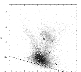
Figure 11: An example of the observed light curve due to a single point mass lensing: the OGLE lens candidate #2 (Udalski et al. 1994a).

Figure 12: The color – magnitude diagram for stars in Baade’s Window. The location of 11 OGLE lens candidates is shown with circles. The dashed line indicates the detection limit applied for the search (Udalski et al. 1994b). The majority of stars are at the main sequence turn – off point of the galactic bulge, near $V-I\approx 1.6$, $V\approx 20$. The bulge red clump stars are near $V-I\approx 1.9$, $V\approx 17$. The disk main sequence stars form a distinct band between $(V-I,V)\approx(1.5,19)$ and $(V-I,V)\approx(1.0,16)$ (Paczyński et al 1994, and references therein).

in the I–band: 93, 187, and 94 in the observing seasons 1993, 1994, and 1995, respectively. The stellar luminosity was constant during these three years, with the average I band magnitude of 19.07, 19.10, and 19.13, respectively; the standard deviation of individual measurements was 0.13, 0.10, and 0.09 magnitude, respectively (M. Szymański, private communication).

The distribution of the OGLE events in the $(V-I)-V$ color – magnitude diagram of the stars seen through Baade’s Window, i.e. at $(l,b)\approx(1,-4)$, is shown in Fig. 12. Note that the events are scattered over a broad area of the diagram populated by galactic bulge stars, in proportion to the local number density of stars multiplied by the local efficiency of event detection (Udalski et al. 1994b). A very similar distribution for over 40 MACHO events detected towards the galactic bulge was shown by Bennett et al. (1995). It is interesting that three out of $\sim 40$ MACHO events appear to be at the location which is occupied by the bulge horizontal branch stars as well as the disk main sequence stars, near $(V-I)\approx 1.2$, $V\approx 17$. Spectroscopic analysis should be able to resolve this ambiguity, i.e. are the lensed stars in the disk or in the bulge.

The most dramatic result is the estimate by the MACHO collaboration that the optical depth to microlensing through the galactic halo is only $9_{-5}^{+7}\times 10^{-8}$ (based on 3 events), and can contribute no more than 20% of what would be needed to account for all dark matter in the halo (Alcock et al. 1995a). The most surprising result is the OGLE discovery that the optical depth is as high as $3.3\pm 1.2\times 10^{-6}$ (based on 9 events) towards the galactic bulge (Udalski et al. 1994b). This result was found independently by MACHO with 4 events (Alcock et al. 1995c), and qualitatively confirmed by DUO (Alard 1996b). It should be remembered that all quantitative analyses of the optical depth as published to date are based on only $16$ events mentioned above. The statistics is improved with the recent preprint (Alcock et al. 1995e) with the analysis of 45 MACHO events detected in the direction of the galactic bulge.

Some nonstandard effects which had been first predicted theoretically were also discovered. These include very dramatic light curves caused by stellar sources crossing caustics created by double lenses (OGLE #7: Udalski et al. 1994d, Bennett et al. 1995, DUO #2: Alard et al. 1995b, and probably one of the MACHO Alert events: Pratt et al. 1996), as predicted by Mao & Paczyński (1991); the paralactic effect of Earth’s orbital motion (Alcock et al. 1995d) as predicted by Gould (1992); the light curve distortion of a very high magnification event by a finite source size (Alcock, private communication) as predicted by Gould (1994a), Nemiroff & Wickramasinghe (1994), Sahu (1994), Witt & Mao (1994), and Witt (1995); the chromaticity of apparent microlensing caused by blending of many stellar sources, only one of them lensed (Stubbs 1995, private communication) as predicted by Griest & Hu (1992).

The first theoretical papers with the estimates of optical depth towards the galactic bulge (Griest et al. 1991, Paczyński 1991) ignored the effect of microlensing by the galactic bulge stars. That effect was noticed to be dominant by Kiraga & Paczyński (1994), who still ignored the fact that there is a bar in the inner region of our galaxy (de Vaucouleurs 1964, Blitz & Spergel 1991). Finally, the OGLE results forced upon us the reality of the bar (Udalski et al. 1994b, Stanek et al. 1994, Paczyński et al. 1994, Zhao et al. 1995, 1996). This “re-discovery” of the galactic bar by the microlensing searchers, who were effectively ignorant of its existence, demonstrates that the microlensing searches are becoming a useful new tool for studies of the galactic structure (Dwek et al. 1995). We are witnessing a healthy interplay between theory and observations in this very young branch of astrophysics.

An example of a dramatic light curve of the first double microlensing event, the OGLE #7, is shown in Fig. 13 for 1992 and 1993 following Udalski et al. (1994d). This star was found to be constant in 1992, 1994, and 1995. The average magnitude based on 32, 45, and 41 I-band measurements in these three observing seasons was 17.53, 17.52, and 17.54, respectively, with the variance of single measurements being 0.07, 0.04, and 0.03 magnitudes, respectively (M. Szymański, private communication). The objects was also found in the MACHO database (Bennett et al. 1995), confirming the presence of the second caustic crossing event near JD 2449200, and demonstrating that the light variation was achromatic.

Figure 13: An example of a binary lensing: the OGLE lens candidate #7 (Udalski et al. 1994d). The region of the two caustic crossings, (a) and (b), is shown enlarged in the two inserts. The MACHO collaboration has a few dozen additional data points in two bands demonstrating that the light variations were achromatic; three MACHO data points cover the second caustic crossing (b) (Bennett et al. 1995).

It is hard to decide which was the first microlensing event, as this depends on what “the first” is supposed to mean. If we take the time at which a microlensing event reached its maximum, then the first was OGLE #10 which peaked on June 29, 1992 (Udalski et al. 1994b). It was followed by six other OGLE events that were observed that summer. However, these were not uncovered until the spring of 1994, when the automated computer searches finally caught-up with the backlog of unprocessed data. The OGLE collaboration discovered its first event, OGLE #1 on September 22, 1993, but it peaked on June 15, 1993, almost a full year later than OGLE #10. The first event to be ever noticed by a human was MACHO #1 – Will Sutherland saw it come out of a computer on Sunday, September 12, 1993 (C. Alcock, private communication). The first three papers officially announcing the first computer detections were published almost simultaneously by EROS (Aubourg et al. 1993), by MACHO (Alcock et al. 1993), and by OGLE (Udalski et al. 1993).

Unfortunately, it is likely that the two events reported by EROS might have been due to intrinsic stellar variability rather than microlensing. EROS #1 has been recently found to be an emission line Be type star (Beaulieu et al. 1995). The MACHO collaboration has identified a new class of variable stars, referred to as bumpers (Cook et al. 1995). These are Be type stars, and it is possible that EROS #1 exhibited a bumper phenomenon. EROS #2 has been recently found to be an eclipsing binary, possibly with an accretion disk (Ansari et al. 1995a). Stars with accretion disks are known to exhibit diverse light variability, and the EROS #2 event might have been due to disk activity. In any case, the fact that both EROS events were related to rare types of stars makes them highly suspect as candidates for gravitational microlensing.

A total of about 100 gravitational microlensing events has been reported so far by the three collaborations: DUO, MACHO, and OGLE. The DUO collaboration reported the detection of 13 microlensing events towards the galactic bulge, one of them double (Alard 1996b, Alard et al. 1995a,b). The MACHO collaboration reported at various conferences a total of about 8 events towards the LMC and about 60 events towards the galactic bulge, and has many more in the data that is still analyzed. The OGLE collaboration has detected 18 events towards the galactic bulge, one of them double. In addition various collaborations confirmed events detected by the others. I am not aware of a single case in which there would be a discrepancy between the data obtained by various collaborations, though there is plenty of difference of opinion about some aspects of the interpretation. Note, that the quantitative analysis of all those $\sim 100$ events lags behind their discovery. Nevertheless, we may expect that robust determinations of the optical depth towards the galactic bulge and towards the LMC will be published in the very near future, as the data is already at hand.

A major new development in the microlensing searches is the on line data processing. The OGLE collaboration implemented its “Early Warning System” (EWS), a full on-line data processing system from the beginning of its third observing season, i.e. from April 1994 (Udalski et al. 1994c). As a result all 8 OGLE events detected in 1994 and 1995 were announced over Internet in real time. The MACHO collaboration, with its vastly higher data rate, implemented the “Alert System” with partial on-line data processing in the summer of 1994 (Stubbs et al. 1995), and full on-line processing by the beginning of 1995 (Pratt et al. 1996). The total number of events detected with the MACHO Alert System as of October 15, 1995 is about 40, and all of them were announced over Internet in real time.

The first papers based on the follow–up of the real time announcements of microlensing events have already been published: Szymański et al. (1994) presented the first light curve of the first event announced by the MACHO Alert System. Benetti et al. (1995) presented the first spectra for the on–going microlensing event.

The implementation of PLANET – Probing Lensing Anomalies NETwork (Albrow et al. 1996) was a major development in 1995. The aim of the project is to follow the announcements of real time detection of microlensing events (currently implemented by the OGLE and MACHO collaborations) with frequent multi-color observations on four telescopes: the Perth Observatory 0.6 m telescope at Bickley, Australia, the 1 m telescope near Hobart in Tasmania, the South African Astronomical Observatory 1.0 m at Sutherland, South Africa, and the Dutch-ESO 0.92 m at La Silla, Chile.

6.2 Data analysis

In order to translate the observed rate of microlensing events into quantitative information about the optical depth and the lens masses it is necessary to calibrate the detection system. This is fairly straightforward, at least in principle, as all data processing is done with computers, with automated software. Naturally, for the calibration to be possible every step of the detection process has to be done according to well defined rules, following the same algorithm for the duration of experiment. The calibration is done by introducing artificial microlensing events into the data stream and using the same algorithm to “detect” them as the one used for real detections. This process can be done at two very different levels: pixels or star catalogs.

If the original data is collected with a CCD camera then from the beginning it is stored in a computer memory in a digital form. Every CCD image obtained by OGLE had $2048\times 2048$ pixels for a total of 8 Megabytes of pixel data. Every MACHO exposure generated 8 such CCD frames, 4 in each of two color bands, for a total of 64 Megabytes. On a clear night between 30 and 100 exposures may be taken. The OGLE collaboration was given $\sim 70$ nights on the Swope 1 meter telescope at the Las Campanas Observatory in Chile (operated by Carnegie Institution of Washington) for each of the four observing season: 1992–95, and generated $\sim 20$ Gb of data every year. The MACHO collaboration refurbished a dedicated 1.3 meter telescope at the Mount Stromlo Observatory in Australia. Their observations began in mid-1992, but the routine operation started in January 1993. Currently, the MACHO collaboration obtains $\sim 800$ Gb of data every year.

If the original data is obtained with photographic plates, as it was done for the main part of the EROS project and the whole DUO project, then the plates have to be scanned and digitized before the data can be stored in a computer memory. A single Schmidt plate has $28,000\times 28,000$ pixels for a total of $\sim 1.6$ Gb of data.

Once the data is available in a form of digital pixel images a dedicated software is used to measure the location and the brightness of stellar images. The MACHO and OGLE collaborations modified DoPhot (Schechter et al. 1993) to make it faster (Udalski et al. 1992, Bennett et al. 1993). The coordinates of stellar images were determined on good CCD frames which were chosen to be the templates. All other frames were first shifted to coincide with the templates using a few bright stars, and the coordinates of all other stars were adopted from the template. Next, the brightness of all template stars was measured on all frames. This speeded the data processing by a large factor, but restricted photometry to those stars which were found on the templates. Also, this procedure makes it impossible to detect proper motions. Using a modified DoPhot software up to $2\times 10^{5}$ stars could be measured on a CCD frame with $\sim 4\times 10^{6}$ pixels, which corresponds to the effective number of $\sim 20$ pixels per star. The DUO software (Alard 1996b, Alard et al. 1995a) measured not only the brightness but also the position of every stellar image on every digitized Schmidt plate, for a total of $\sim 1.4\times 10^{7}$ stars per plate, i.e. $\sim 56$ pixels per star.

The results of stellar photometry are combined into a database of photometric measurements which is searched for microlensing events. Very stringent criteria have to be used for detection because the events are very rare. For example, one of the OGLE conditions was the requirements that at least 5 consecutive measurements of the candidate object had to be brighter than normal, well measured brightness of the star, by more than three standard deviations (Udalski et al. 1994b). This conservative approach was necessary in order not to be swamped with fictitious “events”, but it made the efficiency of the detection rather low. Let $N$ be the total number of photometric measurements of all stars, $n$ the number of microlensing events detected in the database, and $\tau$ be the optical depth to microlensing as estimated on the basis of these detections. Using the published MACHO and OGLE results one finds that $N\tau/n\approx 50-100$. This implies that the effective number of photometric measurement needed for a detection of a single event was $50-100$.

The first catalog level estimate of the efficiency of microlensing detections was published by the OGLE collaboration (Udalski et al. 1994b). It was done introducing artificial microlensing events into the database of photometric measurements and following exactly the same criteria for detection as the criteria used in the original search. It turned out that the efficiency was approximately constant for events in the time scale range 30 days $<t_{0}<$ 100 days, but it dropped rapidly towards shorter time scales: down by a factor 10 at $t_{0}\approx 3$ days and a factor 100 at $t_{0}\approx 1$ day. Very similar results were found by the MACHO collaboration with a much more thorough “pixel level” calibration (Alcock et al. 1995a). In that case the artificial events are added as artificial stars to the images obtained with the CCD detector. This means that the effect of blending of stellar images is automatically taken into account. The pixel level calibration is the correct way to proceed, but it is much more time consuming than the catalog level calibration. Fortunately, the results are the same to within $\sim 20\%$ as the two opposite effects nearly cancel out: stellar blending means that there are really more stars that may be subject to microlensing, and this increases the number of events per stellar image. On the other hand the apparent brightening is reduced making some events impossible to detect.

Note, that as long as the procedure used for the detection of artificial events is exactly the same as the procedure used for the original search, the estimate of the event rate and the optical depth is not influenced in a systematic way by the specific criteria. Naturally, if the criteria are too stringent then there are fewer detections (in the real data as well as in the simulations), and the random errors of the estimated values increase. If the criteria are too lax then in addition to genuine microlensing events a number of intrinsically variable stars, or even artifacts of the detector system, may enter the sample, introducing uncontrollable systematic errors. As far as I know we have no quantitative procedure to define the optimum criteria at this time.

The fact that the current detection systems are sensitive to events over limited range of time scales implies that the estimates of the optical depth and/or the event rates can only provide the lower limits. As the duration of searches increases so does their sensitivity to ever longer events. It will take a different observing procedure to improve the sensitivity to very short events. Most searches done so far made only 1 or 2 photometric measurements per star per clear night. The only CCD search with up to 46 photometric measurements per star per clear night was done by the EROS collaboration, and the null result was reported by Aubourg et al. (1995).

6.3 Consensus and no consensus

There is a consensus now about a number of important issues related to microlensing in our galaxy and near our galaxy. The most important is the consensus that the microlensing phenomenon has been detected. It is not possible to tell at this time what fraction of so called “candidate events” is real, and what fraction is due to poorly known types of stellar variability. My personal guess is that the contamination fraction is probably below 10%, or so. My arguments in favor of microlensing as the dominant source of the newly detected variability are the following:

1. The observed light curves are achromatic, their shapes are well described by simple theoretical formulae.

2. The distribution of magnification factors is consistent with the theoretical expectations (Udalski et al. 1994a), with some events magnified by a factor up to $\sim 100$ (Stubbs 1995, private communication).

3. The double lensing events have been detected, as expected, and roughly at the expected rate.

4. The parallax effect has been detected, as expected.

5. The spectrum of the only event monitored spectroscopically has been found to be constant throughout the intensity variation (Benetti et al. 1995).

6. The galactic bar has been “rediscovered” through the enhanced optical depth.

There is also a consensus on some science issues:

1. The optical depth towards the galactic bulge is large, $\sim 3\times 10^{-6}$.

2. The optical depth towards the LMC is small, $\sim 10^{-7}$.

3. A lot of very interesting science not related to microlensing can be done with huge databases generated with the searches. These include color magnitude diagrams as well as many types of variable stars.

On some issues there is no consensus yet:

1. What is the location of objects which dominate lensing observed towards the galactic bulge? Are these predominantly the galactic bulge stars (Kiraga & Paczyński 1994, Paczyński et al. 1994, Zhao et al. 1995, 1996), or are the lenses mostly in the galactic disk (Alcock et al. 1995c)?

2. What is the dominant location of the objects responsible for the lensing observed towards the LMC? Are these in the galactic disk, galactic halo, the LMC halo, or in LMC itself? Are they stellar mass objects or are they sub-stellar brown dwarfs (Sahu 1994, Alcock et al. 1995a)?

3. What fraction of microlensing events is caused by double lenses?

A consensus on these issues is likely to emerge within a few years, but no doubt new controversies will develop as the volume of data increases.

6.4 Serendipity results

The microlensing searches worked because practical implementation of massive data acquisition and processing systems became possible. These searches generated huge databases of multi band photometry of millions of stars, and lead to the discovery of thousands of variable stars, most of them new. The OGLE galactic bulge variable star catalogues published so far contain full data for 1656 pulsating, eclipsing and other short period variables, including their coordinates and finding charts (Udalski et al. 1994e, 1995a,b). The other OGLE papers include data on RR Lyrae type stars in the Sagittarius dwarf galaxy (Mateo et al 1995b) and Sculptor dwarf galaxies (Kałużny et al. 1995a). The MACHO collaboration presented period – luminosity diagram for $\sim 1500$ cepheids in the LMC and identified 45 double mode pulsators among them (Alcock et al. 1995b), and has a total of $\sim 90,000$ variables in its archive (Cook et al. 1995). The EROS collaboration published data on 80 eclipsing binaries in the LMC (Grison et al. 1995, Ansari et al. 1995a). The DUO collaboration has data on $\sim 15,000$ galactic bulge variables (Alard 1996a). These include $\sim 1,200$ pulsating stars of the RR Lyrae type ab in the galactic bulge, and $\sim 300$ such stars in the Sagittarius dwarf, considerably extending the known size of that galaxy, and clearly demonstrating the usefulness of variable stars as tracers.

Perhaps the most important serendipity result is the discovery by Kałużny et al. (1995b) of the first detached eclipsing binaries at the main sequence turn–off point of the globular cluster Omega Centauri. The follow–up spectroscopic observations will determine, for the first time, the masses of stars at the globular cluster main sequence turn–off point, and hence will provide a sound basis for the reliable age and helium content determinations. The point is that while the theoretical color–magnitude diagrams are affected by our lack of understanding of the mixing length theory, the mass–luminosity relation is insensitive to large changes of the mixing length (Paczyński 1984).

The same detached binaries will allow very accurate determination of distances to globular clusters, while the follow–up spectroscopic observations of the detached eclipsing binaries discovered by the EROS collaboration (Grison et al. 1995) will provide a very accurate distance to the LMC (Paczyński 1996). We may expect that in the near future detached eclipsing binaries will provide accurate distances to all galaxies of the Local Group (Hilditch 1995). It should be pointed out that in order to discover a detached eclipsing binary one needs a few hundred photometric measurements. Only one out of a few thousand stars is of this type, with deep and narrow primary and secondary eclipses, and no anomalies in the light curve. This implies one needs $\sim 10^{6}$ photometric measurements to detect one good system. This is a lot of work, but it will lead to the determination of accurate ages of globular clusters, their helium content, and the Hubble constant, some of the most important numbers for cosmology.

Color-magnitude diagrams obtained in the standard (V,I) photometric system by the OGLE collaboration for the galactic bulge region show evidence for the galactic bar (Stanek et al. 1994). They also indicate that the galactic disk has a low number density of luminous (i.e. massive and young) as well as faint (i.e. low mass and old) main sequence stars in the inner $\sim 4$ kpc (Paczyński et al. 1994), which seems to be consistent with the presence of the strong bar. The color–magnitude diagrams obtained for the recently discovered Sagittarius dwarf allowed Mateo et al. (1995a) to determine the distance of $25.2\pm 2.8$ kpc to this galaxy, and to estimate its age and metallicity to be 10 Gy and [Fe/H] $=-1.1\pm 0.3$, respectively. Alard (1996a) and Mateo et al. (1996) found a large extension of this galaxy by discovering in it a large number of RR Lyrae variables, a by product of massive photometry carried out by DUO and OGLE.

7 The future of microlensing searches

7.1 The near future

The near future of the microlensing searches is easy to predict: more of the same, or rather very much more of the same. While the MACHO collaboration has streamlined its data processing and does it in real time, the EROS and OGLE collaborations are building in Chile their 1-meter class telescopes to be dedicated to massive microlensing searches. Many other groups are either planning or developing new detection systems. In particular, a few groups intend to monitor M31 (Crotts 1992, Ansari et al. 1995b = AGAPE = Andromeda Galaxy and Amplified Pixels Experiment).

It is not known how many stars can be monitored from the ground in the direction of the galactic bulge and all members of the Local Group galaxies, but a fair estimate is $\sim 2\times 10^{8}$, i.e. about one order of magnitude more than the current $\sim 2\times 10^{7}$ of the MACHO collaboration. Note, that stars towards the galactic bulge and towards the LMC and SMC are bright, and even with a 1-meter class telescope the detection limit is set by the crowding of stellar images, not by the sky or the photon statistics. Therefore, the better the seeing the more stars can be detected and accurately measured. It is easily imaginable that within a few years the detection rate will increase to $\sim 300$ events per year towards the galactic bulge and $\sim 10$ events per year towards the LMC and SMC. With $\sim 1000$ events detected towards the bulge, and $\sim 30$ towards the LMC and SMC it will be easy to map the distribution.

The observed distribution of lensing events in the sky will soon reveal the space distribution of the lenses towards the galactic bulge (cf. Evans 1994, Kiraga 1994). A rapid increase of the optical depth towards the center will indicate that the lenses are located predominantly in the bulge of our galaxy. A more or less uniform optical depth will point to the galactic disk as the dominant site of the lensing objects. The task will be more difficult in the case of LMC. The observed rate is low, and it will take longer to accumulate good statistics. A rapid increase of the optical depth towards the center will indicate that the lenses are located predominantly in the bulge of LMC. A more or less uniform optical depth would be more difficult to interpret, as such a result would be compatible with the lenses located either in the galactic disk or in the galactic halo. It may be necessary to measure the optical depth in as many directions as possible, towards all members of the Local Group of galaxies. This is a difficult task as these are far away, and hence their stars are very faint. It is likely that 2-4 meter class telescopes will be required for the observations (Crotts 1992, Colley 1995, Ansari et al. 1995b).

It is interesting to note that the statistics of microlensing of the galactic bulge red clump stars will allow the determination of the geometrical depth of the bulge/bar system (Stanek 1995). The lensed objects will be found predominantly among the stars located on the far side. Therefore, these stars will appear to be fainter, at least on average, than typical red clump stars.

It is likely that within a few years the range of event time scales between 1 hour and 3 years will be very well sampled. With the observed distribution of event time scale known over this whole range, or with stringent upper limits available for some part of the range, it will become meaningful to translate this distribution into the mass function of the lensing events. The necessary pre-requisite will be the knowledge of the space distribution and kinematics of the lenses. It seems safe to expect that the space distribution will be revealed through the variation of the optical depth over the sky, while the kinematics will follow from the improved understanding of the galactic structure. This analysis will not be good enough to know the mass of any particular lens to better than a factor 2 or 3, but it is likely that the overall range of masses will be known with a reasonable accuracy.

There are very many papers and preprints written about the possible distribution of mass within the dark halo, or within the galactic disk, as well as on the possible nature of the lensing objects (those include gas clouds and axion miniclusters). These will not be reviewed here, as I consider them too speculative. A more direct analysis of the data will provide the answers to most interesting current questions in a matter of a few years.

It is virtually certain that the expansion of microlensing searches will be followed with the expansion of the follow-up observations. There is a very natural division of labor in this area as well as in the area of supernovae searches. In order to discover very rare events one needs detectors with as many pixels as possible. The multi–band coverage is not essential. The pixels are expensive and difficult to purchase, and it is practically not possible to fill the whole field of view of a modern 1-meter class telescope with CCDs, as the field may be 1.5 – 5 degrees across. Given a limited number of pixels we have to decide what is more efficient: to put them all in one plane, making the search area as large as affordable, or to cover only 50% of the area in two bands? Note that every detection system is most sensitive in a particular band. For example the OGLE system can record more stellar images in I-band than in V–band in a fixed exposure time. Also, when the moon is bright the sky intensity in the I band is smaller than it is in the V band. Thin CCD chips are currently so expensive that extending the search to the B and U bands is not possible within a realistic budget. The implementation of real–time data analysis, coupled to the distribution of information over the Internet, and the availability of follow-up systems like PLANET (Albrow et al. 1996) makes the multi-band search unnecessary.

On the other hand it is most essential for the follow-up observations to be as multi-band and as frequent as possible. As only a relatively small number of pixels is needed for the follow-up it should be possible to use thin CCD chips for this purpose. A frequent time coverage is most essential as many interesting phenomena happen on the time scale on which a star moves across its own diameter, which takes a few hours. Such source resolving events may allow the measurement of the relative proper motion in the lens–source system (Gould 1994a), as well as to study the structure of stellar photospheres. They may also lead to the detection of planets around stars (Mao & Paczyński 1991).

A dramatic improvement in the data processing software may be expected when the current photometry of stellar images is supplemented with a search for variable point sources using digital image subtraction, also known as “CCD frame subtraction”. The image subtraction is very elegant, and its principles are very simple, as described and implemented by Ciardullo et al. (1990). Imagine that we have two images of the same area in the sky taken under identical seeing conditions, and the same atmospheric extinction. Every point source has an image spread over many pixels according to the point spread function, PSF. When the two images are subtracted from each other there should be no residuals if nothing has changed. If some stars changed their brightness then there should be some residuals, positive or negative, with the profile defined by the PSF. These residuals can be measured, and so the stellar variability can be detected. If we do not care about stars that remain constant then this is by far the most efficient way to proceed. Also, this method may allow the detection of variables which are too crowded to measure the non–variable component of their light due to the constant contaminating stars.

Unfortunately, it is difficult to implement the image subtraction technique, as there are many practical problems as described by Ciardullo et al. (1990). Therefore, it seems reasonable to expect that the proof of its practical usefulness should be provided by the determination of light curves of periodical variables, like pulsating or eclipsing stars. It is much easier to detect a periodic signal, and to confirm its reality, than to detect convincingly a non–periodic and non repeating signal, like a microlensing event. However, the recently published efforts (Crotts 1992, Baillon et al. 1993, Ansari et al. 1995b, Gould, 1995b, 1996) seem to concentrate on the detection of non–periodic signals, referred to as ”pixel lensing”.

7.2 A more distant future

Any discussion of a distant future is obviously speculative, but it is also entertaining. A rather obvious idea is to observe microlensing with space instruments. The natural reasons include stable weather, perfect seeing, and access to the UV and IR. However, there are special advantages for microlensing in putting an instrument at a distance of $\sim 1$ AU from the ground based telescopes, as this would allow to detect the microlensing parallax effect as pointed out by Refsdal (1966) and by Gould (1994b, 1995a). Any observations done at a single site provide only one quantity which has physical significance: the time scale $t_{0}$. Unfortunately, this time scale is a function of the lens mass, its distance, and its transverse velocity (cf. eq. 15), none of which is known. However, the illumination pattern created by the lens varies substantially on a scale of a fraction of the Einstein ring radius, or its projection onto the observer’s plane. Hence, even a small space telescope placed at a solar orbit would reveal a different light curve of the lens, and provide this way some additional information about the lens properties. Unfortunately, this will not be sufficient to solve for all three unknowns. However, if the same event happens to resolve the source then the relative proper motion of the lens–source system can be determined (Gould 1994a), and perhaps a complete solution could be obtained. In particular, the determination of the lens mass might be possible.

There are some problems with this idea. One of them is the high cost, likely to be of the order of $\sim\$10^{8}$, as compared with $\sim\$10^{6}$ for a typical ground based microlensing search (though supposedly “dollars in space weigh less”). Also, even though the parallax effect alone can provide some constraint on the lens, it cannot provide a unique determination of the lens mass, with a possible exception of some special cases, like the very high magnification events during which the source is resolved. Unfortunately, such events are very rare. Perhaps the single most dramatic impact of the space measurements would be a direct proof that a particular event is indeed caused by gravitational microlensing as no other phenomenon can be responsible for the difference in the observed light curves.

Many of the problems, including a decent statistical determination of the lens masses, will be solved in the near future with the ground based observations. When the optical depth to the galactic bulge is mapped with $\sim 10^{3}$ lensing events then the space distribution of the lenses (galactic disk versus galactic bulge/bar) will be definitely understood. As the kinematics of the disk and the bulge/bar stars can be directly observed an adequate model for the lens statistics will be developed as a refinement of the approach outlined in the section 3. Any particular lens is not likely to have its mass determined to better than a factor $\sim 3$ or so, but the average mass, and perhaps the mass range and the slope of the mass function will be deduced. This task will be relatively easy for the lenses observed towards the galactic bulge because of their high rate. It will take much more time to obtain equally reliable information about the lenses observed at high galactic latitudes because of their very low rate. Yet, continuous monitoring of the stars in all Local Group galaxies will provide the basis for the determination of the lens distribution and masses in a matter of a decade or so. This is basically the matter of detecting enough events to map the variation of the optical depth over the sky.

There are at least two cases in which the masses of individual lenses can be measured with no ambiguity. These are lenses belonging to globular clusters seen against the rich stellar background of the galactic bulge or LMC/SMC (Paczyński 1994), and the nearby high proper motion stars seen against the distant stars of the Milky Way or LMC/SMC (Paczyński 1995a). In both cases the distances and proper motions of the lenses can be measured directly, or indirectly (the lenses in the globular clusters will be too dim to see them), and the lens mass remains the only unknown quantity on the right hand side of the eq. (15).

7.3 The limits of ground based searches and the search for planets

The range of lens masses which can give rise to observable lensing events is very broad. At the low end the practical limit is imposed by the finite size of the sources. The amplification of a point source which is perfectly aligned with a lens is infinite (cf. eq. 11 with $u=0$). However, when a source with a finite angular radius $r_{s}$ is perfectly aligned, then its circular disk forms a ring–like image, which has its inner and outer radius, $r_{in}$ and $r_{out}$, given with a slightly modified eq. (9):

$$r_{in}=\left[\left(r_{{}_{E}}^{2}+0.25r_{s}^{2}\right)^{1/2}-0.5r_{s}\right],\hskip 56.9055ptr_{out}=\left[\left(r_{{}_{E}}^{2}+0.25r_{s}^{2}\right)^{1/2}+0.5r_{s}\right],$$

where all quantities are expressed as angles. Assuming, for simplicity, a uniform surface brightness of the source the maximum magnification can be calculated as the ratio of the two areas:

$$A_{max}={\pi r_{out}^{2}-\pi r_{in}^{2}\over\pi r_{s}^{2}}=\left[4\left({r_{{}_{E}}\over r_{s}}\right)^{2}+1\right]^{1/2}.$$

For the event to be reasonably easy to detect we choose $A_{max}\geq\sqrt{2}$, which is equivalent to condition: $r_{s}/r_{{}_{E}}\leq 2$.

An angular radius of a star is given as

$$r_{s}={R_{s}\over D_{s}}=2.3\times 10^{-12}~{}rad~{}\left({R_{s}\over R_{\odot}}\right)~{}\left({10~{}{\rm kpc}\over D_{s}}\right)=0.45~{}\mu sec~{}\left({R_{s}\over R_{\odot}}\right)~{}\left({10~{}{\rm kpc}\over D_{s}}\right).$$

This may be combined with the eq. (13) to obtain

$${r_{s}\over r_{{}_{E}}}=0.00050~{}\left({R_{s}\over R_{\odot}}\right)~{}\left({M_{\odot}\over M}\right)^{1/2}\left({10~{}{\rm kpc}\over D_{s}}\right)\left({D_{d}\over 10~{}{\rm kpc}}\right)^{1/2}\left(1-{D_{d}\over D_{s}}\right)^{-1/2}.$$

The smallest mass for which the Einstein ring radius is no less than half the source radius is given as

$$M\geq M_{min}\approx 6\times 10^{-8}~{}M_{\odot}~{}\left({R_{s}\over R_{\odot}}\right)^{2}~{}\left({10~{}{\rm kpc}\over D_{s}}\right)\left({D_{d}\over D_{s}-D_{d}}\right).$$

If the source is in the galactic bulge, at $D_{s}\approx 8$ kpc, and the lens at $D_{d}\approx 6$ kpc (Zhao et al. 1995, 1996), then condition (54) becomes:

$$M_{min}\approx 2\times 10^{-7}~{}M_{\odot}~{}\left({R_{s}\over R_{\odot}}\right)^{2},\hskip 56.9055pt{\rm(galactic~{}bulge)}.$$

If the source is in the LMC at $D_{s}\sim 55$ kpc, and the lens is in the galactic halo at $D_{d}\sim 10$ kpc then the condition (54) becomes:

$$M_{min}\approx 1.0\times 10^{-7}~{}M_{\odot}~{}\left({R_{s}\over 7~{}R_{\odot}}\right)^{2},\hskip 56.9055pt{\rm(LMC)}.$$

Note that the scaling factor for the source radius is $7~{}R_{\odot}$ in the eq. (56), while it is $R_{\odot}$ in the eq. (55) to allow for the fact that the distance to the LMC is about 7 times larger than to the galactic center, and the source stars near the detection limit are correspondingly larger. The time scale of a microlensing event caused by lenses at the lower mass limit can be calculated combining the eqs. (15), (53) and (54) to obtain:

$$t_{0}\geq 30~{}min~{}\left({R_{s}\over R_{\odot}}\right)~{}\left({D_{d}\over D_{s}}\right)~{}\left({200~{}km~{}s^{-1}\over V}\right).$$

The estimate of $M_{min}$ implies that it should be possible to extend the searches down to masses as small as that of our moon. These objects may be planets lensing together with their parent stars, as described in section 4, or these may be planetary mass objects roaming the interstellar space, rather than orbiting any star. Clearly, the task of finding them will be very difficult unless they are very numerous. Let us make a modest assumption that every star has just one earth mass planet, and a typical mass of the lenses actually responsible for the events detected towards the bulge and the LMC is $\sim 0.3~{}M_{\odot}$. This implies that the mass ratio is $\sim 10^{-5}$, and hence the optical depth to microlensing by those planets is $\sim 3\times 10^{-6}\times 10^{-5}=3\times 10^{-11}$ towards the galactic bulge and $\sim 10^{-7}\times 10^{-5}=10^{-12}$ towards the LMC. These numbers may be somewhat larger as the cross section for planetary microlensing is enhanced by the presence of a nearby star (cf. Figure 9). It is clear that the searches aiming at finding such planets must be vastly more thorough than anything operating now.

Let us make a crude estimate of the most sensitive ground based search for microlensing that could be done by simply making multiple copies of the existing systems. Let all stars that may be microlensed, perhaps $2\times 10^{8}$ of them, be measured every few minutes to detect all events with a time scale $t_{0}\geq 30$ minutes. Let there be $\sim 3000$ hours of clear observing per year combining all ground based sites. This translates into six events per year with $t_{0}\sim 1$ hour if the optical depth is $\tau_{\rm 1~{}hour}\approx 10^{-11}$. The good news is that there are enough stars in the sky to detect a moderately large number of planetary microlensing events with the 1–meter class ground based telescopes if a mega–project is carried out for a few years. The bad news is that the required data rate would be about 1000 times larger than the current MACHO rate. The price tag would certainly be very impressive, but probably not in excess of a single space mission.

This analysis demonstrates that with a rather immodest increase of current microlensing searches the dark objects down to asteroid mass range could be detected even if their fractional contribution to the galactic mass was as small as $\sim 10^{-5}$. It is also possible, at least in principle, to extend the search to masses as large as $10^{5}-10^{6}~{}M_{\odot}$. The events due to lenses that massive have a duration of $\sim 100$ years, yet they may be detected, at least in principle, with two very different methods. First, a parallax effect due to Earth orbital motion will introduce $\sim 1\%$ modulation in the light curve, with a period of one year (Gould 1992). Second, very numerous stars which are normally below the detection threshold will be occasionally microlensed by a very large factor. According to the eq. (11) the highly magnified source is within factor of 2 of its peak brightness for a time interval $t_{1/2}=t_{0}\sqrt{3}/A_{max}$, which may be reasonably short for $A_{max}\geq 100$ (Paczyński 1995b). So, either of the two methods may allow the extension of the microlensing searches to the range of supermassive MACHOs.

8 Acknowledgments

It is a great pleasure to acknowledge the discussions with, and comments by Drs. C. Alcock, D. Bennett, J. Kałużny, A. Kruszewski, M. Kubiak, S. Mao, J. Miralda-Escudè, M. Pratt, K. Sahu, K. Z. Stanek, C. Stubbs, M. Szymański, A. Udalski, and J. Wambsganss. This work was supported by the NSF grants AST-9216494 and AST-9313620.

References

- (1) Abt, H. 1983, Annu. Rev. Astron. Astrophys. 21:343
- (2) Alard, C. 1996a, Ap. J. 458:L17
- (3) Alard, C. 1996b, in Proc. IAU Symp. 173, p. 215 (Eds. C. S. Kochanek, J. N. Hewitt; Kluwer Academic Publishers, Dordrecht/Boston/London)
- (4) Alard, C., Guibert, J., Bienayme, O., Valls-Gabaud, D., Robin, A. C. et al. 1995a, The Messenger, No. 80, p. 31
- (5) Alard, C., Mao, S., Guibert, J. 1995b, Astron. Astrophys. Lett. 300:L17
- (6) Albrow, M., Birch, P., Caldwell, R., Menzies, J., Sackett, P. D. et al. 1996, in Proc. IAU Symp. 173, p. 227 (Eds. C. S. Kochanek, J. N. Hewitt; Kluwer Academic Publishers, Dordrecht/Boston/London)
- (7) Alcock, C., Allsman, R., Axelrod, T., Bennett, D., Cook, K. et al. 1993, Nature 365:621
- (8) Alcock, C., Allsman, R., Axelrod, T., Bennett, D., Cook, K. et al. 1995a, Phys. Rev. Lett. 74:2867
- (9) Alcock, C., Allsman, R., Axelrod, T., Bennett, D., Cook, K. et al. 1995b, Astron. J. 109:1653
- (10) Alcock, C., Allsman, R., Axelrod, T., Bennett, D., Cook, K. et al. 1995c, Ap. J. 445:133
- (11) Alcock, C., Allsman, R. A., Alves, D., Axelrod, T. S., Bennett, D. P. et al. 1995d, Ap. J. 454:L125
- (12) Alcock, C., Allsman, R. A., Alves, D., Axelrod, T. S., Bennett, D. P. et al. 1995e, preprint: astro-ph/9512146
- (13) Ansari, R. 1995, Nuclear Phys. B (Proc. Suppl.) 43:108
- (14) Ansari, R., Cavalier, F., Couchot, F., Moniez, M., Perdereau, O., et al. 1995a, Astron. Astrophys. Lett. 299:L21
- (15) Ansari, R., Auriére, M., Baillon, P., Bouquet, A., Coupinot, G., et al. 1995b, Nuclear Phys. B (Proc. Suppl.) 43:165
- (16) Aubourg, E., Bareyre, P., Bréhlin, S., Gros, M., Lachiéze-Rey, M., et al. 1993, Nature 365:623
- (17) Aubourg, E., Bareyre, P., Bréhin, S., Gros, M., de Kat, J. et al. 1995, Astron. Astrophys. 301:1
- (18) Baillon, P., Bouquet, A., Giraud-Héraud, Y., and Kaplan, J. 1993, Astron. Astrophys. 277:1
- (19) Beaulieu, J. P., Ferlet, R., Grison, P., Vidal-Madjar, A., Kneib, J. P. et al. 1995, Astron. Astrophys. 299:168
- (20) Benetti, S., Pasquini, L., West, R. M. 1995, Astron. Astrophys. Lett. 294:L37
- (21) Bennett, D. P., Rhie, S. H. 1996, preprint: astro-ph/9603158
- (22) Bennett, D. P., Akerlof, C., Alcock, C., Allsman, R., Axelrod, T., et al. 1993, Annals of the NY Acad. Sci. 688:612
- (23) Bennett, D. P., Alcock, C., Allsman, R., Axelrod, T., Cook, K. H., et al. 1995, AIP Conf. Proc. 336: “Dark Matter” (Eds.: S. S. Holt, D. P. Bennett), p. 77
- (24) Black, D. C. 1995, Annu. Rev. Astron. Astrophys. 33:359
- (25) Blandford, R. D., Narayan, R, 1992, Annu. Rev. Astron. Astrophys. 30:311
- (26) Blitz, L., Spergel, D. N. 1991, Ap. J. 379:631
- (27) Bolatto, A. D., Falco, E. E. 1994, Ap. J. 436:112
- (28) Butler, R. P., Marcy, G. W. 1996, preprint
- (29) Chang, K., Refsdal, S. 1979, Nature, 282:561
- (30) Ciardullo, R., Tamblyn, P., Phillips, A. C. 1990, Publ. Astron. Soc. Pac. 102:1113
- (31) Colley, W. N. 1995, Astron. J. 109:440
- (32) Cook, K. H., Alcock, C., Allsman, R., Axelrod, T., Freeman, K., et al. 1995, in Proc. IAU Colloquium 155, ASP Conf. Ser. 83: “Astrophysical Applications of Stellar Pulsations”, p. 221 (Ed. R. Stobie)
- (33) Crotts, A. P. S. 1992, Ap. J. Lett. 399:L43
- (34) de Vaucouleurs, G. 1964, IAU Symp. 20: The Galaxy and the Magellanic Clouds, (Eds.: F. J. Kerr, A. W. Rotgers), 195
- (35) De Rújula, A., Jetzer, Ph., and Massó, E. 1991, Monthly Notices of the Royal Astronomical Society 250:348
- (36) Di Stefano, R., Esin, A. A. 1995, Ap. J. Lett. 448:L1
- (37) Di Stefano, R., Mao, S. 1996, ApJ, 457:93
- (38) Dwek, E., Arendt, R. G., Hauser, M. G., Kelsall, T., Lisse, C. M., et al. 1995, Ap. J. 445:716
- (39) Dyson, F. W., Eddington, A. S., Davidson, C. R. 1920, Mem. Royal Astronomical Society 62:291
- (40) Einstein, A. 1911, Annalen der Physik 35:898
- (41) Einstein, A. 1916, Annalen der Physik 49:769
- (42) Evans, N. W. 1994 Ap. J. Lett. 437:L31
- (43) Gott, R. J. 1981, Ap. J. 243:140
- (44) Gould, A. 1992, Ap. J. 392:442
- (45) Gould, A. 1994a, Ap. J. Lett. 421:L71
- (46) Gould, A. 1994b, Ap. J. Lett. 421:L75
- (47) Gould, A. 1995a, Ap. J. Lett. 441:L21 Gould, A. 1995b, Ap. J. 455:44
- (48) Gould, A. 1996, in Proc. IAU Symp. 173, p. 365 (Eds. C. S. Kochanek, J. N. Hewitt; Kluwer Academic Publishers, Dordrecht/Boston/London)
- (49) Gould, A., Loeb, A. 1992, Ap. J. 396:104
- (50) Griest, K. 1991, Ap. J. 366:412
- (51) Griest, K., Alcock, C., Axelrod, T. S., Bennett, D. P., Cook, K. H. et al. 1991, Ap. J. Lett. 372, L79
- (52) Griest, K., Hu, W. 1992, Ap. J. 397:362
- (53) Grison, P., Beaulieu, J-P., Pritchard, J. D., Tobin, W., Ferlet, R., et al. 1995, Astron. Astrophys. Suppl. 109:447
- (54) Hilditch, R. W. 1995 “Binaries in Clusters”, ASP Conf. Ser. (Eds. G. Milone and J.-C. Mermilliod) in press
- (55) Kałużny, J., Kubiak, M., Szymański, M., Udalski, A., Krzemiński, W., Mateo, M. et al. 1995a, Astron. Astrophys. Suppl. 112:407
- (56) Kałużny, J., Kubiak, M., Szymański, M., Udalski, A., Krzemiński, W. et al. 1995b, “Binaries in Clusters”, ASP Conf. Ser. (Eds. G. Milone and J.-C. Mermilliod) in press
- (57) Kamionkowski, M. 1995, Ap. J. 442:L9
- (58) Kayser, R., Schramm, T., Nieser, L. (Editors) 1992, “Gravitational Lenses” (Lecture Notes in Physics 406, Springer-Verlag)
- (59) Kiraga, M. 1994, Acta Astron. 44:241
- (60) Kiraga, M., Paczyński, B. 1994, Ap. J. 430:101
- (61) Kochanek, C. S., Hewitt, J. N. (Editors) 1996, “Astrophysical Applications of Gravitational Lensing”, Proc. IAU Symposium 173: Kluwer Academic Publishers, Dordrecht/Boston/London)
- (62) Lynds, R., Petrosian, V. 1989, Ap. J. 336:1
- (63) Mao, S., Di Stefano, R. 1995, Ap. J. 440:22
- (64) Mao, S., Paczyński, B. 1991, Ap. J. Lett. 374:L37
- (65) Mao, S., Paczyński, B. 1996 Ap. J., submitted = astro-ph/9604002
- (66) Marcy, G. W., Butler, R. P. 1996, preprint
- (67) Mateo, M., Udalski, A., Szymański, M., Kałużny, J., Kubiak, M., Krzemiński, W. 1995a, Astron. J. 109:588
- (68) Mateo, M., Kubiak, M., Szymański, M., Kałużny, J., Krzemiński, W., Udalski, A. 1995b, Astron. J. 110:1141
- (69) Mateo, M., Mirabel, N., Udalski, A., Szymański, M., Kałużny, J., et al. 1996, Ap. J. 458:L13
- (70) Mayor, M. and Queloz, D. 1995, Nature, 378:355
- (71) Mellier, Y., Fort, B., Soucail, G. (Editors) 1990, “Gravitational Lensing” (Lecture Notes in Physics 360, Springer-Verlag)
- (72) Moran, J. M., Hewitt, J. N., Lo, K. Y. (Editors) 1989, “Gravitational Lenses” (Lecture Notes in Physics 330, Springer-Verlag)
- (73) Nemiroff, R. J. and Wickramasinghe, W. A. D. T., 1994, Ap. J. Lett. 424:L21
- (74) Paczyński, B. 1984, Ap. J. 284:670
- (75) Paczyński, B. 1986a, Ap. J. 301:503
- (76) Paczyński, B. 1986b, Ap. J. 304:1
- (77) Paczyński, B. 1991, Ap. J. Lett. 371:L63
- (78) Paczyński, B. 1994, Acta Astron. 44:235
- (79) Paczyński, B. 1995a, Acta Astron. 45:345
- (80) Paczyński, B. 1995b, Acta Astron. 45:349
- (81) Paczyński, B. 1996, in Proc. IAU Symp. 173, p. 199 (Eds. C. S. Kochanek, J. N. Hewitt; Kluwer Academic Publishers, Dordrecht/Boston/London)
- (82) Paczyński, B., Stanek, K. Z., Udalski, A., Szymanński, M., Kałużny, J. et al. 1994, Ap. J. Lett. 435:L113
- (83) Pratt, M. R., Alcock, C., Allsman, R. A., Alves, D., Axelrod, T. S. et al. 1996, in Proc. IAU Symp. 173, p. 221 (Eds. C. S. Kochanek, J. N. Hewitt; Kluwer Academic Publishers, Dordrecht/Boston/London)
- (84) Refsdal, S. 1964, MNRAS 128:295
- (85) Refsdal, S. 1966, MNRAS 134:315
- (86) Refsdal, S., Surdej, J. 1994, Rep. Prog. Phys. 56:117
- (87) Sahu, K. 1994, Nature 370:275
- (88) Roulet, E., Mollerach, S. 1996, Physics Reports, in press = astro-ph/9603119
- (89) Schechter, P. L., Mateo, M., Saha, A. 1993, Publ. Astron. Soc. Pac. 105:1342
- (90) Schneider, P., Ehlers, J., Falco, E. E. 1992, “Gravitational Lensing” (Berlin: Springer Verlag)
- (91) Schneider, P., Weiss, A. 1986, Astron. Astrophys. 164:237
- (92) Soldner, J. 1801, Berliner Astronomisches Jahrbuch 1804, p. 161
- (93) Stanek, K. Z., Mateo, M., Udalski, A., Szymański, M., Kałużny, J., Kubiak, M. 1994, Ap. J. 429:L73
- (94) Stanek, K. Z. 1995, Ap. J. 441:L29
- (95) Stubbs, C., Alcock, C., Cook, K., Allsman, R., Axelrod, T., et al. 1995, Bulletin American Astron. Soc. 26, 1337
- (96) Surdej, J., Fraipont-Caro, D., Gosset, E., Refsdal, S., Remy, M. (Editors) 1993, “Gravitational Lenses in the Universe” (Proc. 31st Liege Coll.)
- (97) Szymański, M., Udalski, A., Kałużny, J., Kubiak, M., Krzemiński, W., Mateo, M. 1994, Acta Astron. 44:387
- (98) Udalski, A., Szymański, M., Kałużny, J., Kubiak, M., Mateo, M. 1992, Acta Astron. 42:253
- (99) Udalski, A., Szymański, M., Kałużny, J., Kubiak, M., Krzemiński, W. et al. 1993, Acta Astron. 43:289
- (100) Udalski, A., Szymański, M., Kałużny, J., Kubiak, M., Mateo, M., Krzemiński, W. 1994a, Ap. J. 426:L69
- (101) Udalski, A., Szymański, M., Stanek, K. Z., Kałużny, J., Kubiak, M. et al. 1994b, Acta Astron. 44:165
- (102) Udalski, A., Szymański, M., Kałużny, J., Kubiak, M., Mateo, M. et al. 1994c, Acta Astron. 44:227
- (103) Udalski, A., Szymański, M., Mao, S., Di Stefano, R., Kałużny, et al. 1994d, Ap. J. Lett. 436:L103
- (104) Udalski, A., Kubiak, M., Szymański, M., Kałużny, J., Mateo, M., Krzemiński, W. 1994e, Acta Astron. 44:317
- (105) Udalski, A., Szymański, M., Kałużny, J., Kubiak, M., Mateo, M., Krzemiński, W. et al. 1995a, Acta Astron. 45:1
- (106) Udalski, A., Olech, A., Szymański, M., Kałużny, J., Kubiak, M. et al. 1995b, Acta Astron. 45:433
- (107) Walsh, D., Carswell, R. F., Weymann, R. J. 1979, Nature 279:381
- (108) Witt, H. 1993, Ap. J. 403:530
- (109) Witt, H. 1995, Ap. J. 449:42
- (110) Witt, H., Mao, S. 1994, Ap. J. 430:505
- (111) Wolszczan, A. 1994, Science 264:538
- (112) Wolszczan, A., Frail, D. A. 1992, Nature 355:145
- (113) Zhao, H. S., Spergel, D. N., Rich, R. M. 1995, Ap. J. Lett. 440:L13
- (114) Zhao, H. S., Spergel, D. N., Rich, R. M. 1996, MNRAS, in press
- (115) Zwicky, F. 1937, Phys. Rev. 51:290