Near-infrared and optical broadband surface photometry of 86 face-on disk dominated galaxies.

1 Introduction

For many years broadband colors have been used to obtain a basic insight into the contents of galaxies. Broadband photometry is relatively easy to obtain and gives an immediate impression of the spectral energy distribution (SED) of an object. Broadband colors are particularly efficient when used for statistical investigations such as this one. Colors have been used to estimate the stellar populations of galaxies (e.g. Searle et al.[1973]; Tinsley[1980]; Frogel[1985]; Peletier[1989]; Silva & Elston[1994]) and it has been suggested that colors can give information about the dust content of galaxies (Evans[1994]; Peletier et al.[1994], [1995]). In this paper I use radial color profiles to investigate the stellar and dust content of galaxies.

The problem of determining the stellar content of galaxies from integrated SEDs has been approached from two sides, often called the empirical and the evolutionary approach (for a review, see O’Connell[1987]). In the first method, stellar SEDs are fitted to the observed galaxy SEDs (Pickles[1985]; Peletier[1989]). This method works only if one has spectral (line) information. Generally, the broadband colors of a galaxy can be explained by a combination of the SEDs of two or three types of stars (Aaronson[1978]; Bershady[1993]). In the second, more theoretical approach, stellar SEDs are combined, using some knowledge of initial conditions and evolutionary time scales of different stellar populations, to produce evolutionary stellar population synthesis models (for reviews Tinsley[1980]; Renzini & Buzzoni[1986]; more recent models are e.g. Buzzoni[1989]; Bruzual & Charlot[1996]; Worthey[1994]).

The papers of Disney et al.([1989]) and Valentijn([1990]) have renewed the debate on whether spiral galaxies are optically thick or thin. Broadband colors of galaxies can be used to examine this problem, because the dependence of dust extinction on wavelength causes reddening. This can be used to measure extinction at a certain point through the disk using a galaxy or another object behind it (Andredakis & van der Kruit[1992]) or to measure extinction within a galaxy, for instance across a spiral arm dust lane (Rix & Rieke[1993]; Block et al.[1994]). To measure the global dust properties of a galaxy by reddening one can use the color profile. If one assumes that dust is more concentrated towards the center (just like the stars), the higher extinction in the center produces a color gradient that makes galaxies redder inwards (Evans[1994]; Byun et al.[1994]).

Most previous studies investigating stellar population and dust properties of galaxies used their integrated broadband colors. The use of surface photometry colors is less common, as it is easier to compare integrated photometry than surface photometry for large samples of galaxies. Integrated photometry samples the bulk properties of galaxies, but because the light distribution of galaxies is strongly concentrated, one effectively measures the colors of the inner regions of galaxies. The half total light radius of an exponential disk is $\sim$1.7 scalelengths, while luminosity profiles are easily traced out to 4-6 scalelengths. Therefore, half of the light in integrated colors comes from an area that is less than $1/5$ of the area commonly observed in galaxies (say within $D_{25}$).

Our knowledge of the star formation history (SFH) and the dust content of galaxies improves when we start looking at local colors instead of integrated colors. A first improvement is obtained by using the radial color distribution (i.e. the color profile) of a galaxy. This has been common practice for elliptical galaxies (e.g. Peletier et al.[1990a]; Goudfrooij et al.[1994]), but not for spiral galaxies, because elliptical galaxies are assumed to have a simple SFH and low dust content (but see Goudfrooij[1994]) opposed to spirals. Color studies of spiral galaxies have been concentrated on edge-on systems, in the hope to be better able to separate the dust and stellar population effects (e.g.Just et al.[1996]). Even more detailed information about galaxies can be obtained by the use of azimuthal profiles (Schweizer[1976]; Wevers et al.[1986]) and color maps, but these techniques require high resolution, high signal-to-noise observations and are hard to parameterise to global scales, which means that they cannot be used in statistical studies.

Due to the large variety of galaxies, statistical studies of galaxies require large samples. The introduction of CCDs into astronomy made it possible to obtain for large samples of galaxies accurate optical surface photometry in reasonable observing times (Kent[1984]). Very large data sets of CCD surface photometry have recently become available (Cornell[1987]; Han[1992]; Mathewson et al.[1992]; Giovanelli et al.[1994]). Unfortunately, most of these samples are observed in only one or two passbands. Furthermore, the surface photometry is often reduced to integrated magnitudes and isophotal diameters to study extinction effects with an inclination test or to study the Tully-Fisher relation (Tully & Fisher [1977], hereafter TF-relation). Fast plate measuring machines have also produced surface photometry of large sets of galaxies (e.g.Lauberts & Valentijn[1989], hereafter ESO-LV), but again only in one or two passbands.

Since near-infrared (near-IR) arrays have become available only in the late eighties, near-IR surface photometry is available for only a few somewhat larger samples of spiral galaxies. Terndrup et al.([1994]) observed 43 galaxies in $J$ and $K$, which was complemented with $r$ passband photometry of Kent([1984], [1986], [1987]). They explained the observed colors mainly by population synthesis and invoked dust only for the reddest galaxies. Peletier et al.[1994] imaged 37 galaxies in the $K$-passband and combined their data with the photometry of the ESO-LV catalog. They explained their surface photometry predominantly in terms of dust distributions and concluded that spiral galaxies are optically thick in the center in the $B$ passband, under the assumption that there are no population gradients across the disk.

There are two sets of observations that allow a direct physical interpretation of color gradients in spiral galaxies: 1) The current star formation rate (SFR) as measured by the H$\alpha$ flux has a larger scalelength than the underlying older stellar population (Ryder & Dopita[1994]). There are relatively more young stars in the outer regions of spiral galaxies than in the central regions. This will be reflected in broadband colors of spiral galaxies. 2) From metallicity measurements of H ii regions it is known that there are clear metallicity differences in the gas among different galaxies and that there are metallicity gradients as function of radius within galaxies (Villa-Costas & Edmunds[1992]; Zaritsky et al.[1994]). If the metallicity gradients in the gas are also (partly) present in the stellar components, the effects might be observable in the broadband colors. Stellar population synthesis models incorporating both age and metallicity effects are needed in the comparison with observations of radial color gradients.

Broadband photometry is often assumed to trace baryonic mass, and the transformation from light to mass is performed by postulating a mass-to-light ratio ($M/L_{\lambda}$). Both dust extinction and differences in stellar populations will influence $M/L_{\lambda}$ ratios, most notably in the bluer optical passbands. Color differences, among galaxies and locally within galaxies, will translate in different $M/L_{\lambda}$ values; one can expect that this will influence studies involving rotation curve fitting and the TF-relation.

In this paper I concentrate on the use of color profiles as a diagnostic tool to investigate dust and stellar content of spiral galaxies. Other processes that may contribute to the broadband colors (e.g. emission from hot dust in the $K$ passband) are ignored as they are expected to be small in most cases. The structure of this paper is as follows. In Sect.2 the data set is described and the color profiles of the 86 spiral galaxies using the $B,V,R,I$ and $K$ passband data are presented. Section3 describes the extinction models and the stellar population models used in this paper and then compares these models to the data. In Sect.4, I investigate the relation between the color properties of the galaxies and the structural galaxy parameters derived in the previous papers of this series. Implications of the current measurements are discussed in Sect.5 and the paper is summarized in Sect.6.

2 The data

Fig. 1.: Observed color profiles for 8 out of the 86 galaxies. The dashed lines indicate the maximum error due wrong sky background subtraction, the arrow indicates one disk scalelength in the $K$ passband.

In order to examine the parameters describing the global structure of spiral galaxies, 86 face-on systems were observed in the $B,V,R,I,H$ and $K$ passbands. A full description of the observations and data reduction can be found in de Jong & van der Kruit ([1994], hereafter PaperI) of which only the essentials are repeated here. The galaxies in this statistically complete sample of undisturbed spirals were selected from the UGC (Nilson [1973]) to have red diameters of at least 2^′ and axis ratios larger than 0.625. The galaxies were imaged along the major axis with a GEC CCD on the 1m Jacobus Kapteyn Telescope at La Palma in the $B,V,R$ and $I$ passbands and with a near-IR array on the United Kingdom Infra-Red Telescope at Hawaii in the $H$ and $K$ passbands. Standard reduction techniques were used to produce the images, which were calibrated using globular cluster standard star fields. The sky brightness was determined outside the galaxy in areas free of stars and its uncertainty constitutes one of the main sources of error in the derived parameters.

Fig. 2.: The average $B$–$K$ colors of all galaxies at different radii as function of the azimuthally averaged $R$ passband surface brightness measured at these radii. The galaxies are divided into the four indicated RC3 morphological type index (T) bins. The dashed lines give a common reference in all four bins, but have no physical meaning. The lines have a $B$–$K$ color gradient of 1/7 mag per $R$-mag arcsec^-2.

The ellipticity and position angle (PA) of each galaxy were determined from the $R$ passband image at an outer isophote (typically at 24 $R$-mag arcsec^-2). The radial surface brightness profiles were determined for all passbands by calculating the average surface brightness on elliptical annuli of increasing radius using the previously determined ellipticity and PA. This method ensures that the luminosity profile reflects the average surface brightness at each radius, independent of passband. Free ellipse fitting at each surface brightness interval (e.g.Kent[1984]) will give a disturbed representation of the radial luminosity distribution in face-on galaxies, due to spiral arms, bars and bright H ii regions. The surface brightness profiles were used to calculate the integrated luminosity of the galaxies. Internal and external comparisons showed that the derived parameters are well within the estimated errors.

The decomposition of the light of the galaxies into its fundamental components (bulge, disk and sometimes a bar) is described by de Jong ([1996a], hereafter PaperII). An exponential light distribution was assumed for both the bulge and the disk and these were fitted to the full 2D image. An extensive error analysis of the determination of the fundamental galaxy parameters was performed and this revealed that the dominant source of error is the uncertainty in the sky background.

The color profiles of the galaxies were calculated by subtracting the radial surface brightness profiles of the different passbands from one another. Some typical profiles are presented in Fig.1, the profiles of all galaxies can be found in de Jong([1995]) and are available in electronically readable format. The dashed lines indicate the maximum errors due to the uncertainty in the sky surface brightness. One should be cautious in interpreting the colors in the inner few seconds of arc, because the profiles were not corrected for the differences in seeing (PaperI) between the different passbands.

A quick inspection shows that almost all galaxies show color gradients. They become bluer going radially outward, even when taking the sky background subtraction uncertainties into account. The color gradients extend over several disk scalelengths. Note that bulges leave no clear signature in the color profiles. From the color profiles alone one can not tell which part is bulge dominated and which part is disk dominated.

The profiles in Fig.1 are the observed profiles. The corrections needed to translate observed quantities into more physical quantities are discussed by de Jong ([1996b], hereafter PaperIII). In the remainder of this paper, only the photometric observations are used, corrected for Galactic extinction using the precepts of Burstein and Heiles ([1984]) and the extinction curve of Rieke and Lebofsky ([1985]).

3 Color gradients

The color gradients of Fig.1 have been put on a common scale in Fig.2, where I have plotted for all galaxies the average $B$–$K$ color at each radius as function of the azimuthally averaged $R$ passband surface brightness at the corresponding radii. The galaxies are divided in four bins based on their morphological type, using the RC3 (de Vaucouleurs et al.[1991]) type indices T (see also PapersI and III). There is a clear correlation between average surface brightness at a radius and the average color at that radius; the lower surface brightness regions are bluer. This indicates the relation between Hubble type, surface brightness and integrated color: since late-type galaxies have on average a lower central surface brightness (PaperIII), they are bluer. This is not the whole story, since for each morphological type at each surface brightness there is considerable scatter. Furthermore, even at the same average surface brightness, late-type galaxies are on the average bluer than early-type galaxies.

The two most straightforward explanations for the color gradients are 1) radial changes in stellar populations and 2) radial variations in reddening due to dust extinction. For both possibilities, I investigate a range of models to limit the acceptable parameter space. The extinction models have a range in relative distributions of dust and stars. The colors of the stellar synthesis population models depend on the star formation history (SFH) and the metallicity of the stars.

The colors and color gradients of the galaxies formed from the different passband combinations are correlated and the models should be fitted in a six-dimensional “passband space”. Predicting the right color gradient in one combination of passbands, but a wrong one in an other combination makes a model at best incomplete and therefore undesirable. Color–color plots will be used to show as much information as possible in one plot. The $H$ passband data are not shown, as the differences between $H$ and $K$ predicted by the models (both the population and the extinction models) are smaller than the measurement errors. In the remainder of this section I first discuss the extinction models and the stellar population synthesis models used in this paper and then compare the models with the data.

3.1 Extinction models

In this section, I present my new dust models, show the predicted luminosity profiles, color profiles and color–color diagrams, and compare the results with existing dust models.

3.1.1 Modeling dust effects

Numerous researches have investigated the effects of dust extinction on the observed light distributions of galaxies. The primary goal of most of the studies is to investigate the inclination dependent effects of the total magnitude of galaxies (e.g. Huizinga[1994]). In some studies the extinction effects on the observed (exponential) light profile of galaxies is studied. The most detailed are the Triplex models by Disney, Davies & Phillipps ([1989], hereafter DDP; see also Huizinga[1994]; Evans[1994]).

The effects of reddening on the observed colors and color profiles has been examined in a number of studies. The simplest model to predict the reddening of a galaxy is to use directly the standard (Galactic) extinction law, but this is of course a gross oversimplification. DDP have named this the Screen model, which has all dust placed between us and the galaxy. In reality the dust is mixed between the stars, so that on the near side of the galaxy a considerable fraction of stars will be only slightly obscured. For the same amount of dust, the observed reddening is considerably less than predicted by the Screen model, especially since the most reddened stars are also the most obscured stars and therefore the ones that contribute less to the overall color of the system.

As soon as the dust is mixed with the stars one has to take both absorption and scattering into account. Intuitively one expects that for face-on galaxies at least as much light gets scattered into the line of sight as out of it, especially since there are more photons traveling in the plane of a galaxy which can be scattered into face-on directions than the other way around. As only the absorbed photons really disappear, it is better to use relative absorption rather than relative extinction between different passbands to estimate reddening effects in face-on galaxies. It is essential to incorporate both absorption and scattering into extinction models to make accurate predictions of the effects of dust on colors and color gradients of galaxies.

A number of studies have investigated the effect of reddening on integrated colors of galaxies (Bruzual et al.[1988]; Witt et al.[1992] and references therein). In these studies scattering is included and stellar and dust distributions are used that allow approximations to reduce computing time; e.g. Bruzual et al. use plane parallel distributions and Witt et al. use spherically symmetric distributions. Color profiles produced by dust models are not often presented. Evans ([1994]) investigates the effects of extinction as function of radius in face-on galaxies for a non-scattering medium. Byun et al.([1994]) also investigate the effects of dust on luminosity and color profiles, using the method of Kylafis & Bahcall ([1987]). Their method includes first order scattering and approximates multiple scattering. The results of Byun et al.[1994] are compared with the results presented here in Sect.3.1.2.

To estimate to what extent the color gradients can be attributed to reddening by dust extinction, Monte Carlo simulations were made of light rays traveling through a dusty medium. The models are described in full detail in AppendixA.

The distributions of stellar light and dust in these models were described by exponential laws in both the radial and vertical directions. In the radial direction these distributions were parameterised by the scalelength of the stars ($h_{\rm s}$) and the dust ($h_{\rm d}$), and in vertical direction by the scaleheight of stars ($z_{\rm s}$) and dust ($z_{\rm d}$). In all models I used $h_{\rm s}/z_{\rm s}\!=\!10$ and for simplicity no bulge component was added to the stellar light distribution.

Since the effects of dust on the color profiles is the main interest of this study, absolute calibration of the amount of starlight is arbitrary. Only the relative effect of dust from one passband to the other is important. The amount of dust in the models is parameterised by the optical depth of a system, $\tau_{0,V}$, defined as the optical thickness due to dust absorption and scattering in the $V$ passband through the disk from one pole to the other along the symmetry axis (Eq.(A16)).

Fig. 3.: The relative extinction ($\tau_{\lambda}/\tau_{V}$) and the relative extinction ($(1-a_{\lambda})\tau_{\lambda}/\tau_{V}$) used in the dust models.

Three dust properties were incorporated into the dust model to describe the wavelength dependent effects of dust extinction: the relative extinction ($\tau_{\lambda}/\tau_{V}$), the albedo ($a_{\lambda}$), and the scattering asymmetry parameter ($g_{\lambda}$). The relative extinction was adopted from Rieke and Lebofsky ([1985]); the other two parameters were drawn from Bruzual et al.([1988]). These values are listed in Table1 and Fig.3 shows the relative extinction and the relative absorption ($(1-a_{\lambda})\tau_{\lambda}/\tau_{V}$). Note that for the optical passbands the change in relative absorbtion is much smaller than the change in relative extinction.

passband	$\tau_{\lambda}/\tau_{V}$	$a_{\lambda}$	$g_{\lambda}$
$U$	1.531	0.68	0.67
$B$	1.324	0.66	0.59
$V$	1.000	0.60	0.50
$R$	0.748	0.53	0.40
$I$	0.482	0.45	0.29
$H$	0.175	0.28	0.04
$K$	0.112	0.20	0.00

Table 1.: Values used in the scattering model for the dust properties relative extinction ($\tau_{\lambda}/\tau_{V}$), albedo ($a_{\lambda}$) and scattering asymmetry ($g_{\lambda}$) as function of photometric passband.

Before presenting the model results, a few words of caution are in order. First, extragalactic dust properties are poorly known. There are only a few measurements of extinction laws in extragalactic systems (e.g. Knapen et al.[1991]; Jansen et al.[1994]) other than for the Magellanic Clouds (see Mathis[1990] for references). All measurements seem to be consistent with the Galactic extinction law, except for a few measurements in the Small Magellanic Cloud. It is well known that the Galactic extinction curve is not the same in all directions, but the one adopted here is appropriate for the diffuse interstellar medium (for discussion see Mathis[1990]). The parameters $a_{\lambda}$ and $g_{\lambda}$ have never been measured in extragalactic systems and are poorly known even for our own Galaxy. The adopted values for these parameters stem, especially for the longer wavelengths, from model calculations. Still, no large variations are expected in the extinction properties, unless the dust in other galaxies is made of totally different material (see also the discussion in Bruzual et al.[1988]).

As a second word of caution, the models presented here describe only smooth diffuse dust. The effects of non-homogeneous dust distributions should be considered. A large ensemble of optically thick clouds has only a reddening effect if the clouds have a large filling factor, but such a configuration becomes comparable to the presented models with high $\tau_{0,V}$. The reddening effect of a clumpy medium will be smaller than the effect predicted by the diffuse dust models for the same amount of dust, but the direction of the reddening vectors will be the same as long as the dust properties in the clouds are more or less the same as used here. If clouds are optically thick at all wavelengths one has the case of gray dust and no color gradients at all. Model calculations using a clumpy dust medium in the absence of scattering are presented in Huizinga ([1994], Chapter5).

As a final word of caution, a young population of stars probably has a smaller scaleheight than an old population of stars. It might be more appropriate to use a smaller stellar scaleheight in the blue than in the near-IR. The relative contributions from young and old populations are difficult to estimate however, and for simplicity one stellar scaleheight is used for all passbands. These models do not include the dust shells around the extremely luminous stars in the final stages of their life. Even though such shells will make these stars redder, they will not produce a radial effect (unless the shell properties depend on galactic radius). Effectively these shells will only make the total underlying population redder at all radii and they are of no further concern here.

3.1.2 Resulting profiles

Fig. 4.: The surface brightness (top) and color (bottom) as function of radius resulting from the Monte Carlo dust simulations of face-on galaxies. The radius is units of disk scalelength. The central optical depth and dust to stellar scalelength and scaleheight ratios are indicated top right. The dashed lines indicate unobscured $B$ and $K$ passband profiles. The luminosity profiles have an arbitrary offset and are from top to bottom the $K$, $H$, $I$, $R$, $V$, $B$ and $U$ passband profiles. The color profiles are plotted under the assumption that the underlying color indices are zero, and are from top to bottom ($B$–$K$), ($B$–$H$), ($B$–$I$), ($B$–$R$), ($B$–$V$) and ($B$–$U$).

Fig. 4.: -continued.

Figure4 shows luminosity and color profiles resulting from the Monte Carlo simulations. The luminosity profiles for the different passbands have been given an arbitrary offset and the dust free cases of the $B$ and the $K$ passbands are indicated by the dashed lines. The color profiles have been plotted under the arbitrary assumption that the underlying stellar populations have color indices of zero in all passband combinations. The noise in the color profiles is due to the statistical processes inherent to Monte Carlo simulations.

The luminosity profiles of the $h_{\rm d}/h_{\rm s}\!=\!1$ models show deviations from the unobscured profiles only at the inner two scalelengths. These deviations are quite small except for the highest $\tau_{0,V}$ values. The differences between the different $z_{\rm d}/z_{\rm s}$ models are also quite small and are only apparent for the high $\tau_{0,V}$ values. The gradients can be large in $B$–$H$ and $B$–$K$, but are in general smaller than 0.3 mag in the other color combinations. The color gradients are small in the wavelength range from the $U$ to the $R$ passband, because the absorption properties do not differ very much among these passbands. The change in scattering properties causes the differences in extinction in this wavelength range.

The luminosity profiles for the $h_{\rm d}/h_{\rm s}\!=\!2$-3 models are affected over several scalelengths by dust extinction. In fact, the $h_{\rm d}/h_{\rm s}\!=\!3$, $\tau_{0,V}\!=\!10$-20 models are optically thick over almost the entire disk. The result is that the profiles stay exponential, but with a lower surface brightness and a slightly different scalelength from the unobscured case. The color profiles show no color gradients for these models, only color offsets. The typical surface brightness is produced at $\tau_{\lambda}\!=\!1$ over the entire disk, and the color offsets reflect that different wavelengths probe different depths into the galaxy.

To my knowledge, the models of Byun et al.[1994] are the only models in the literature that have exponential light and dust distributions, and include scattering to calculate luminosity and color profiles. These models can be compared to the models presented, but only indirect, because Byun et al. defined the optical depth of a system differently. They parameterize the optical depth of a system as the absorption in the $V$ passband through the whole disk of a face-on galaxy along the symmetry axis, while here the extinction is used (Eq.(A16)). Furthermore, they use the Galactic extinction law to translate the absorption coefficient from one passband to another. Using Table1 one can calculate that their $\tau_{V}(0)$ models corresponds to my $\tau_{0,V}\!=\!\tau_{V}(0)/(1\!-\!a_{\lambda})$ models, which is 2.9$\tau_{V}(0)$ for the $B$ passband and 1.8$\tau_{V}(0)$ for the $I$ passband. It is probably most meaningful to compare the $\tau_{0,V}\!=\!20$, $z_{\rm d}/z_{\rm s}\!=\!0.3$, $h_{\rm d}/h_{\rm s}\!=\!1$ $B$ passband profile of Fig.4 with the bulgeless (BT0.0), face-on $\tau(0)\!=\!5.0$ profile of their Fig. 7. The central extinction of slightly more than 1 mag and the general shape of the luminosity profile (which is unaffected by extinction for radii larger than 2-3 scalelengths) are comparable. Their $B$–$I$ color profiles are physically not very plausible, because they use the Galactic extinction curve instead of an absorption curve to translate their absorption coefficients from one passband to another. A comparison of the color profiles is therefore not meaningful. Their luminosity profiles can be used, but note that their $\tau_{V}(0)$ should be divided by (1–$a_{V}$) to get the extinction suffered by a point source behind the galaxy, as done here.

What is the range of plausible model parameter values? Quite high $\tau_{0,V}$ and/or $h_{\rm d}/h_{\rm s}$ values are needed to explain the observed $B$–$K$ color gradients of one magnitude over five scalelengths (Fig.1) by dust reddening alone. On the other hand, models with equal scaleheight for dust and stars need an additional dust component, because these models do not produce a clear dust lane in edge-on galaxies. It is also unlikely on dynamical grounds that the dissipational dust and the dissipationless stars have the same scaleheight. Kylafis & Bahcall ([1987]) find a dust-to-star scaleheight ratio of 0.4 in their best fitting model of edge-on galaxy NGC 891 and the dominant dust component is expected to have a $z_{\rm d}/z_{\rm s}$ ratio between 0.3 and 0.5.

The high $h_{\rm d}/h_{\rm s}$ models are favored by Valentijn ([1990], [1994]), who concluded from inclination tests that Sb-Sc galaxies have a $\tau_{B}\!\sim\!1$ through the disk at $D_{25}$. This extinction at about 3-4 stellar scalelengths translates to $\tau_{0,V}\!\sim\!20$ models, if the dust density is distributed exponentially with $h_{\rm d}/h_{\rm s}\!=\!1$. The edge-on extinction from the center out to 3-4 stellar scalelengths gives at least $\tau_{V}\!\approx\!50$ in such a model, which is in conflict with observations of edge-on galaxies. A few edge-on galaxies have been imaged in the near-IR indicating $A_{V}\!\approx\!8$-10 (Wainscoat et al.[1989]; Aoki et al.[1991]), and the Galactic center can be seen in the $K$ passband (Rieke & Lebofsky[1985], $A_{V}\!\approx\!30$ and $A_{K}\!\approx\!3$). Thus $\tau_{0,V}\!=\!20$ models represent extremely dusty galaxies, and certainly no galaxies with $\tau_{0,V}$$\geq$20 are expected. If one increases $h_{\rm d}/h_{\rm s}$ to 3, $\tau_{0,V}$ has to be 2-4 to get $\tau_{V}\!=\!1$ through the disk at 3 stellar scalelengths. This then gives an edge-on $\tau_{V}\!=\!20$-40 from the center out to 3 stellar scalelengths when using large $z_{\rm d}/z_{\rm s}$ values, which are the most favorable for these models. Therefore, the edge-on extinction values of the $\tau_{0,V}\!=\!2$-4, $h_{\rm d}/h_{\rm s}\!=\!3$ models are marginally consistent with the observations, but these models do not produce very large color gradients.

3.1.3 Resulting color–color diagrams

Fig. 5.: Color–color plots resulting from dust models of face-on galaxies. The color zero-points are arbitrary (depending on the color of the underlying stellar population) and are indicated by the filled circles. The centers of the model galaxies are indicated by the open circles and the colors are followed in radial direction for four and a half scale lengths. The solid lines are the results from the Monte Carlo simulations, described in AppendixA. The dotted lines are the results from the DDP models, using the Galactic absorption law rather than the extinction law between the different passbands. The reddening vectors in the top right corners indicate the Galactic extinction law (i.e. Screen model).

Four color–color plots of dust models are presented in Fig.5. Because extinction is a relative measurement, the zero-point can be chosen freely in these plots; only the shapes of the profiles are fixed. The solid lines show the results from the Monte Carlo simulations. The dotted lines are the result of the Triplex models of DDP. To calculate the $\tau_{0}$ for the DDP models in the different passbands, the indicated $\tau_{0,V}$ values were multiplied by $(\tau_{V}/\tau_{\lambda})(1-a_{\lambda})/2$ (Table1). This is equivalent to using an absorption law rather than an extinction law between the different passbands. The factor 2 arises because the DDP models are characterized by the optical depth from the galaxy center to the pole and not by the optical depth through the whole disk.

Comparing the results from the Monte Carlo simulations with the DDP models, one can see that the models agree remarkably well for high optical depths. The intuitive idea that just as many photons are scattered out of the line of sight as are scattered in seems correct for face-on galaxies. Photons are only lost due to absorption. For low optical depths the reddening almost completely disappears. Once a photon gets scattered into the line of sight, the chances of it getting absorbed or scattered again are minimal; even bluing instead of reddening can occur. Even though the amount of reddening is a strong function of the dust configuration, it seems that the direction of the reddening vector is largely dependent on the dust properties. Obviously the reddening produced by these models is different from the reddening produced by a Screen model with the Galactic extinction law (also indicated in Fig.5).

In conclusion, dust can produce color gradients in face-on galaxies, but this requires quite high central optical depths and preferably long dust scalelengths. The reddening vectors of realistic dust models that include both absorption and scattering are completely different from the often-used Screen model extinction models.

3.2 Evolutionary stellar population synthesis models

Ever since the invention of the concept of stellar populations in galaxies (Baade[1944]), numerous models have been made to predict the integrated light properties of such populations and thus of galaxies as a whole. Initially the empirical approach was often followed, in which the different contributions of the stellar populations are added to match the observed galaxy SED. Later, knowledge about initial conditions and stellar evolution were added to make evolutionary synthesis models. This section contains a brief description of population synthesis models, concentrating on the synthesis models used here, followed by a description of the effects that star formation history (SFH) and metallicity have on the colors produced by synthesis models.

3.2.1 Modeling stellar populations

Fig. 6.: Evolutionary color–color plots of stellar synthesis models. The symbols indicate the number of years after creation of this population. To the right in each panel, the different ages connected by solid lines, are the single burst models of Worthey ([1994]) for different metallicities. The corresponding [Fe/H] values are indicated next to them. To the left in each panel are the solar metallicity models of Bruzual & Charlot ([1996]). The dotted line indicates the single burst evolution. The dashed line is a model with an exponentially declining star formation rate. The leftmost dot-dashed line, overlapping the blue part of the exponentially declining SFR model, indicates a model with constant star formation. Bruzual & Charlot used the Johnson $R$ and $I$ passbands which were here converted to Kron-Cousins $R$ and $I$ passbands using the equations of Bessell([1979]).

In recent years a large number of synthesis methods have appeared in the literature, all of which require many input parameters (Tinsley[1980]; Renzini & Buzzoni[1986]; Worthey[1994] and references therein). The simplest models use a initial mass function (IMF) to create a single burst of stars, whose evolution in time is then followed. Slightly more complicated models describe the star formation rate (SFR) in time. In the most complicated models, the gas, stellar, and chemical evolution are linked and described in a self-consistent way. This last type of model has not been used here, since to date only a small range of SFHs have been investigated with these models. The description of the evolution alone does not produce an SED and therefore the models are linked to a stellar library to calculate the evolution in time of the integrated passband fluxes or of the integrated spectrum.

The results from the models in the literature are not all in agreement. The disagreements arise mainly from differences in the treatment of the late stages of stellar evolution. The models do agree on the two main parameters determining the integrated colors of a synthesized galaxy. First of all the colors are strongly determined by the colors of the youngest population, thus by the SFH, and secondly the colors are considerably affected by the metallicities of the populations. In Sect.1 it was noted that both these SFH and metallicity changes have been observed on a radial scale in spiral galaxies. Furthermore, the radial age and metallicity gradients in our own Galaxy are well known and have been extensively studied (Gilmore et al.[1989]; Matteucci[1989], [1992] and references therein). Synthesis models incorporating both age and metallicity effects are needed in the comparisons with spiral galaxy data.

The population synthesis models of Bruzual & Charlot ([1996], BC96 models hereafter, see also Charlot & Bruzual[1991]; Bruzual & Charlot ([1993]) and of Worthey([1994], W94 models hereafter) are used in the remainder of this paper; they are shown in the color–color diagram of Fig.6. The BC96 models used here are based on the isochrone tracks of the Padova group (Bressan et al.[1993]) and on an empirical stellar flux library. The BC96 isochrone synthesis approach makes calculation of the very early stages of evolution of a population possible. The W94 models are constructed from the isochrones of VandenBerg([1985]) and the Revised Yale Isochrones (Green et al.[1987]) and use a theoretical stellar flux library. A different approach was followed in the BC96 and W94 models to calculate the integrated spectra of an evolving stellar population, but the main difference of interest here is the regions of age-metallicty parameter space that were investigated. The BC96 models were only calculated for solar metallicity, but give colors of populations as young as 1.26$\times 10^{5}$ yr. The W94 models span a wide range in metallicity, but the youngest population is 1.5 Gyr.

The models used here were calculated with the standard Salpeter IMF (Salpeter[1955]), with lower mass cutoff at 0.1 $M_{\odot}$ and upper mass cutoff at 2 $M_{\odot}$ (W94) or 100 $M_{\odot}$ (BC96). The use of other solar neighborhood type IMFs or other cutoffs has only small effects compared to the main factors determining the colors of a synthesized population, namely age (or SFH) and metallicity. The main result will be some shifts of the colors in color–color space. Using IMFs deviating strongly from the solar neighbourhood IMF will result in substantial changes, but without strong evidence these types of IMFs are hard to justify.

A comparison study of several stellar population synthesis models has been performed by Charlot, Worthey & Bressan([1995], hereafter CWB). They find substantial discrepancies among the models, especially in $V$–$K$, which are larger than the typical observational errors for galaxies. They conclude that age determinations from galaxy colors are about 35% uncertain at a given metallicity and 25% uncertain in metallicity at a given age, even for a single burst population. The main source of disagreement stems from differences in the stellar evolution prescription, with a smaller component resulting from the spectral calibrations. For comparison, to see the effect of other stellar evolutionary tracks, de Jong ([1995], [1996c]) presents a similar color–color analysis as presented here, but using Bruzual & Charlot ([1993]) with Maeder & Meynet ([1991]) evolutionairy tracks instead of BC96 with Padova tracks.

The W94 and B96 models were chosen to cover a large age-metallicity space, but given the uncertainties in the models, any other set of up-to-date set of models could have been chosen (e.g.Bressan, Chiosi & Fagotto[1993]; von Alvensleben & Gerhard[1994]). The particular choice of models will not change the main results of this study. The model uncertainties will mainly result in the uncertainty of absolute calibration of colors, but the relative color trends are reasonably correct. With the current state of modeling, I will only indicate which regions in galaxies and what type of galaxies are younger/older or have higher/lower metallicity.

3.2.2 Star formation history in color–color diagrams

Three evolutionary tracks of the BC96 models are shown in Fig.6. The simplest is the single burst model, in which the color evolution of one initial starburst is followed in time. In the other two tracks this single burst model has been convolved in time to yield color evolution for different SFHs. In one model an exponentially declining SFR with a time scale of 5 Gyr was used, in the other model the SFR was held constant. These models show the importance of the very early stages of stellar evolution. The constant SFR model at 17 Gyr is as blue in $B$–$V$ and $B$–$I$ as the exponentially declining model at 8 Gyr and the single burst model at 1.5 Gyr! Still, a solar metallicity starburst cannot produce colors to the right of the indicated single burst line in Fig.6, because the colors of very young populations (age $<$1.5 Gyr, not shown) all lie to the left of (or in the direction of) the single burst trend.

3.2.3 Age and metallicity in color–color diagrams

Of the W94 models, only the single burst models of different metallicities are shown in Fig.6. The synthesis method of W94 prevents calculation of the very early evolution stages of a stellar population. Young populations are especially hard to synthesize for the lower metallicities, simply because there are no young, low metallicity stars in the solar neighborhood that can be used as input stars for the models.

The lower metallicity populations of the W94 models are clearly bluer in all color combinations. Age and metallicity are not complete degenerate. The offset in optical–near-IR colors is slightly larger than the offset in optical–optical colors. A low metallicity system can be recognized by its blue $V$–$K$ or $R$–$K$ color with respect to its $B$–$V$ and $B$–$I$ colors. When mixing populations of different age and metallicity the model grid points can be more or less added as vectors and then age and metallicity are degenerate. An individual galaxy can never be pinpointed to a certain age and metallicity using broadband colors.

Fig. 7.: The $B$–$V$ versus $R$–$K$ color–color plots of the program galaxies divided into the four morphological type bins indicated at the bottom-right of the panels. The centers of the galaxies are indicated by the open circles; the thin lines follow the color profiles in radial direction in steps of 1 $K$ passband scalelength. At the bottom-left of the 0$\leq$T$<$3 panel, the typical rms error in the zero-point calibration is indicated. Some of the dust models of Sect.3.1 are plotted in the top-left of the panels. The thick dashed lines in the center of the panels connect the 17 Gyr and the 8 Gyr points of the BC96 models presented in Sect.3.2. In the 5$\leq$T$<$6 panel the 12 Gyr single burst W94 models for different metallicities are connected, the marks indicate the [Fe/H] values. The thick solid lines in the 6$\leq$T$\leq$10 panels represent the W94 models. Points of equal metallicity, but different age are connected.

Fig. 8.: Same as Fig.7, but for $B$–$I$ versus $V$–$K$.

The single burst BC96 and W94 models are clearly offset from each other. The solar metallicity BC96 model lies somewhere in between the [Fe/H] $\!=\!-0.25$ and [Fe/H] $\!=\!0.0$ W94 models. These are the kinds of differences between models that were studied in detail by CWB, resulting mainly from uncertainties in stellar evolutionairy tracks. The relative trends agree reasonably well, confirming that it is allowed to look the relative trends in color space. The BC96 models will be mainly used to investigate trends in SFH, because contrary to the W94 models, they incorporate the very early stages of stellar evolution. To compare with the data, I will connect the 8 Gyr points of the different SFH BC96 models and do the same for the 17 Gyr points. These connected data points will indicate the color trends for equally old populations with different SFHs. The W94 models have to be used to look at the effects caused by metallicity, because different metallicities are not available in the BC96 models.

3.3 Color gradients; measurements versus models

In this section I first use color–color diagrams to display the observations. I then try to explain the observed color gradients by comparing these measurements with the dust models, the different SFH synthesis models, and finally the full population synthesis models, that incorporate both age and metallicity effects.

3.3.1 The measurements in color–color diagrams

The color–color profiles of the galaxies are presented in Figs7 and8. The data were smoothed to reduce the noise in the profiles. The first data point (at the open circle) is the average over the inner half scalelength (in the $K$ passband) of the luminosity profiles, the other points are averages moving outward in steps of one $K$ scalelength. The uncertainty of the inner point is dominated by the zero-point uncertainty of the calibration and is indicated at the bottom of the top-left panels of Figs7 and8. In the blue direction of the color–color profiles, lower surface brightnesses are traced (see Fig.2) and errors are dominated by sky background uncertainties. Strange kinks at the blue ends of the profiles should thus not be trusted.

The profiles of galaxies with T$<$6 are confined to a small region in the color–color plots. The colors between different passband combinations are strongly correlated. The scatter is slightly larger than the average zero-point error. The central colors of the galaxies become on average a little bit bluer going from T=0 to T=6, but they follow the main trend.

The galaxies with morphological classification T$\geq$6 clearly deviate from the main trend. Their central colors range from the normal red to extreme blue, even bluer than the bluest outer parts of the earlier type galaxies. The spread in the color–color diagram is also significantly larger for the late-type galaxies. Some of the late-type galaxies have very blue $V$–$K$ and $R$–$K$ colors for their $B$–$V$ and $B$–$I$ colors, especially when compared to the earlier types.

When comparing models with the data one should realize that as soon as a model for a galaxy has been chosen, it should be applied to all color combinations. In particular, the same model should be used in both Figs7 and 8. It is tempting to propose one single model for all galaxies, because the profiles are confined to a small region in the diagrams. We only need to explain the offsets from the main trends with additional parameters.

3.3.2 Measurements versus dust models

The reddening profiles produced by the dust models are indicated on the left in the panels of Figs7 and 8. The color of the underlying stellar population is arbitrary and thus the dust profile can be placed anywhere in the diagram. The dust models have a distinct direction in the color–color diagrams independent of the dust configuration, as explained in Sect.3.1. This direction is clearly different from the general trend of the data and therefore the whole gradient cannot be produced by the dust reddening alone. A small fraction of the color gradients could be due to dust reddening, but an additional component is needed to explain the full gradient.

This does not mean that there could not be large amounts of dust, but rather that the color gradients are not mainly caused by dust reddening. If the dust is not diffuse, but strongly clumped into clouds the amount of reddening is strongly reduced. It could be that a large fraction of the most luminous stars is embedded in dust clouds. This will not induce a color gradient or an inclination dependent extinction effect, but will give the total color profile an offset in the general direction of the calculated dust models. The “dusty nucleus” models of Witt et al.([1992]) give an even better indication of the expected offset vector if the luminous stars are embedded in dust clouds.

3.3.3 Measurements versus metallicity effects

To what extent can metallicity differences in the stellar populations account for the color gradients? The 12-Gyr-old W94 single burst models for different metallicities are connected in the 5$\leq$T$<$6 panels of Figs7 and8. Models at other ages follow the same direction in color space. The single-age, different-metallicity model does not match the data for most of the galaxies. Again another component is needed to explain the color gradients; radial metallicity differences alone are not sufficient. It is important to note that population models cannot be arbitrarily shifted, they predict fixed colors for a given SFH and metallicity.

3.3.4 Measurements versus star formation history

The BC96 models are indicated by dashed lines in Figs7 and8. The 8 Gyr points of the models have been connected as well as the 17 Gyr points. The reddest ends of these lines indicate single burst models, the bluest ends represent constant SFR models. In between is a model with an exponentially decreasing SFR with a time scale of 5 Gyr. The color vector of the T$<$6 systems seem to be reasonably well matched by the BC96 models, but most galaxies are offset to the blue in the $V$–$K$ and $R$–$K$ colors. The offset is the smallest for the 8 Gyr model, but then most of the galaxy centers are even redder than predicted by the single burst model. Because we know that galaxies still have star formation in their centers, this is an unlikely situation. As mentioned before, model uncertainties allow for some shifts in these diagrams, but the most likely conclusion has to be that although SFH variations as function of radius are a good driving force for radial color gradients, alone they cannot explain the full color gradients. This is especially true for the galaxies with T$\geq$6, which certainly have $V$–$K$ and $R$–$K$ colors too blue to be explained by the solar metallicity BC96 models.

3.3.5 Measurements versus age and metallicity effects

The W94 models in the 6$\leq$T$\leq$10 panel indicate that the very blue galaxies in this panel can be described very well by low-metallicity population synthesis models. As with the earlier type galaxies, the radial color trends are reasonably well described by age differences, but at all radii lower metallicities are needed for most of the galaxies. A number of them are so blue in all color combinations that their stellar components must be young and of low metallicity.

Galaxies are known to have radial metallicity gradients in their current gas content (Villa-Costas & Edmunds[1992], hereafter VE; Zaritsky et al.[1994], hereafter ZKH), and have radial SFRs that are not linearly correlated with their radial stellar surface brightness, which means they do not have one SFH as function of radius (Ryder & Dopita[1994]). As long as there are no consistent stellar population synthesis models that incorporate very young stellar evolutionary stages at all metallicities, it is difficult to make quantitative statements about the observed colors and color gradients of the galaxies.

Limits can be set on the models using the metallicity measurements collected by VE and ZKH. Recall that metallicity measurements yield the current gas metallicities in H ii regions, so that the underlying stellar component could have completely different metallicity values. For galaxies T$<$6 the 12+log(O/H) values run from $\sim$9.3 in the center to $\sim$8.6 at $R_{25}$. The O/H indices of later type galaxies are a few tenths lower, from about 8.9 to 8.2, but with more or less the same gradient across the disk. Using log(O/H)${}_{\odot}\!\simeq\!-3.08$ (Grevesse & Anders[1989]) and [O/Fe] $\simeq\!0.1$$\sim$0.5 (e.g. Wyse & Gilmore[1988]) the O/H values can be transformed to [Fe/H] values and used with the W94 models. The [Fe/H] values run from about a central 0.2 to –0.6 in the outer regions in galaxies with T$<$6, and from approximately –0.1 to –1.1 in the later type galaxies.

The metallicities just calculated should not be taken too literally in the comparison of the W94 models with the data in Figs7 and 8. As noted before, models should be used to indicate trends in color–color space but cannot be expected to give absolute colors in an individual galaxy. Still, the $B$–$V$ and $B$–$I$ colors are far too red at each radius using the 12 Gyr W94 models in the metallicity range determined from the H ii regions ([Fe/H] = 0.2 to -0.6). This must mean that either the underlying stellar populations have a much lower average metallicity than the surrounding gas or that at each radius a much younger stellar population is present, making the average age lower than 12 Gyr. In the center, the contribution of the young stars cannot be very large, because the color vector of SFH (indicated for solar metallicity by the BC96 models) is in the wrong direction from the (t=12 Gyr, [Fe/H] = 0.25) point in the 5$\leq$T$<$6 panel. Therefore the center probably contains a mix of populations of different metallicities, with an average metallicity far lower than the current metallicity of the surrounding gas ([Fe/H] $\simeq$ 0.2), but on average higher than the gas metallicity of the outer regions. Towards the outer parts of galaxies, the SFH color vector gives an excellent description of the observed color trend. In the outer regions it is unlikely that the metallicity of the stars is much higher than that of the gas for all galaxies, and the metallicity of the stars must be of the order [Fe/H] = -0.6 (-1.1 for the late types) or less. Thus the color gradients are probably driven by a combination of SFH and metallicity differences as function of radius. The outer parts of galaxies are clearly younger on average than the central regions. If part of the color gradients is also caused by reddening, the age effect must even be larger, because this is the only effect that has a color vector that can compensate the dust color vector.

In conclusion, the centers of spiral galaxies with T$<$6 contain probably a relatively old population of stars, with a range in metallicities. The populations in the outer regions are on average much younger and their metallicity is probably lower, as the gas metallicity is much lower than the metallicity needed to explain the central colors. Overall, later type galaxies have lower metallicity, and a number of them are dominated by very young, low-metallicity populations. The observed color gradients cannot be caused by reddening alone, if the dust properties used in the models are more or less correct. Likewise, metallicity gradients cannot cause the color gradients on their own, the color vectors are in the same direction as the dust model vectors, but as metallicity gradients are observed in the gas, it is likely they are present in the stars as well. Age gradients across the disk have to be even larger if reddening or metallicity gradients are important. It should be noted that the population models can predict both the right colors and the right color gradients within one system of models, while the dust models can at best explain only the color gradients.

4 Colors and the structural galaxy parameters

Most of the information that can be extracted from the galaxy colors of this data set is contained in the previous sections, but for most data sets such detailed radial color information is not available. In order to allow comparisons with these other data sets, a number of relationships between colors and fundamental galaxy parameters are shown in this section.

In the previous section I argued that color gradients derived from different passband combinations are correlated in such a way that stellar population differences seem to be the most reasonable explanation of the phenomenon. Figure2 suggests that the slope of the color gradient has a universal value for all galaxies, but this is an oversimplification.

Fig. 9.: The difference in scalelength between the different passbands. Only points with errors smaller than 0.15 are plotted. Different symbols are used to denote the indicated morphological types.

The change in scalelength ($h^{\lambda}$) as function of passband can be used to parameterise color gradients in the disk. The bulge/disk decomposition technique and the method used to determine the central surface brightnesses and scalelengths for the current data set were described in PaperII. A trivial recalculation shows that each axis of Fig.9 indicates approximately the color change per scalelength in the relevant passband combinations. This figure illustrates again that color gradients are correlated, but also that there is no universal value for the gradient for all galaxies. The values range from about 0.1 to –0.8 mag per scalelength in $B$–$K$.

The change in scalelength was used to find correlations between the steepness of the color gradient and other structural galaxy parameters. A large number of structural parameters were investigated, but none of them showed a correlation with color gradient. The parameters investigated include: inclination, morphological type, central surface brightness, scalelength, bulge-to-disk ratio, integrated magnitude, integrated colors, bulge color, bar versus non-bar, H i and CO fluxes, far-infrared IRAS fluxes and colors, group membership and rotation velocity. Fluxes at the different wavelengths normalized by area or integrated $K$ passband flux were also used in the correlations, but with a negative result. A weak correlation was found only between the steepness of the color gradient and the central color of the disk.

Fig. 10.: The Galactic reddening corrected integrated $B$–$I$ colors of the galaxies as function of morphological type index. The crosses show the values averaged over the bins indicated by the horizontal bars. The vertical bars are the standard deviations on the mean values. Only the galaxies with an error of less than 0.5 mag in their color were used.

In the literature integrated colors of galaxies are usually used to determine galaxy properties. The integrated colors as function of type are presented in Table2 for this galaxy sample and the $B$–$I$ colors are plotted in Fig.10. There is a clear correlation between type and color, but the scatter is large. The integrated color of a galaxy is dominated by the color of the central region and even though color correlates with (central) surface brightnesses (Fig.2), one should note that each morphological type comes in a range of central surface brightnesses (PaperIII) which then explains the large scatter in the integrated colors. It is better to determine and compare the colors of galaxies at a fixed isophote when looking for correlations.

Fig. 11.: The central surface brightness $B$–$K$ color of the disk versus the effective surface brightness $B$–$K$ color of the bulge. Different symbols are used to denote the indicated morphological type ranges. The dashed line indicates the line of equality.

In Fig.11, the central bulge and disk colors of the galaxies are compared. The colors of bulge and disk are clearly correlated. This could be expected, as most color profiles show no clear changes in color gradient in the bulge region. Excluding the three deviant points with bulge $B$–$K$ colors bluer than 2 mag, the bulge is on average 0.14$\pm$0.55 mag redder in $B$–$K$ than the central disk color, which means that the stellar populations probably do not differ very much.

5 Discussion

An important consequence of the color differences in and among galaxies is the implied change in the $M/L_{\lambda}$ values. The comparison of the data with the dust and stellar population models indicates that the color gradients in the galaxies of this sample result mainly from population changes and that dust reddening only plays a minor role. The $M/L_{\lambda}$ values corresponding to the synthesis models presented in Figs7 and8 are listed in Table3.

RC3 type	#	$B$–$V$	#	$B$–$R$	#	$B$–$I$	#	$B$–$H$	#	$B$–$K$
0$\leq$T$\leq$2	7	0.81 $\pm$ 0.19	10	1.35 $\pm$ 0.22	8	1.83 $\pm$ 0.31	6	3.46 $\pm$ 0.21	10	3.75 $\pm$ 0.28
2$<$T$\leq$4	14	0.74 $\pm$ 0.13	26	1.20 $\pm$ 0.19	24	1.78 $\pm$ 0.23	6	3.14 $\pm$ 0.34	26	3.53 $\pm$ 0.28
4$<$T$<$6	19	0.67 $\pm$ 0.15	19	1.20 $\pm$ 0.13	20	1.75 $\pm$ 0.10	10	3.28 $\pm$ 0.14	21	3.51 $\pm$ 0.26
6$\leq$T$<$8	11	0.59 $\pm$ 0.21	11	1.06 $\pm$ 0.26	12	1.61 $\pm$ 0.23	3	2.96 $\pm$ 0.62	8	3.18 $\pm$ 0.45
8$\leq$T$\leq$10	4	0.69 $\pm$ 0.14	5	1.10 $\pm$ 0.10	5	1.44 $\pm$ 0.24	0	—	4	2.99 $\pm$ 0.09

Table 2.: The integrated colors for different morphological type ranges using only the photometric observations of PaperI with errors in the colors less than 0.5 mag. The # lists the number of galaxies in each subsample.

In every passband, young populations have much lower $M/L_{\lambda}$ values than old populations. Young populations still contain very massive stars, which are very luminous for their mass, but expend their energy quickly. Continually adding in young populations, as done in the exponentially declining and constant SFR BC96 models, decreases the $M/L_{\lambda}$ values drastically. Young massive stars are blue so that this effect is most pronounced in the $B$ passband. The change in $M/L_{B}$ is about a factor of 6-11 between the 2 and 17 Gyr for both the BC96 and the W94 models and $M/L_{B}$ changes a factor of 3-5 between the single burst and the constant SFR BC96 models.

Metallicity has an entirely different effect on the $M/L_{\lambda}$ ratios. The $M/L_{B}$ values increase with metallicity, while the $M/L_{K}$ values decrease with metallicity. The turnover point is somewhere between the $I$ and the $J$ passband. This was the motivation for W94 to recommend the $I$ passband for standard candle work and for studies of $M/L$ in galaxies.

The recommendation of the $I$ passband is not entirely obvious, because the choice of optimum passband depends on whether one expects extinction, age or metallicity to have the largest influence on the photometry. If extinction is expected to play a role, the $K$ passband should be used, as the extinction in the $K$ passband is $\sim$4 times less than the extinction in the $I$ passband. The $K$ passband should also be preferred if differences in SFR are expected to be important; see for instance the change in $M/L_{\lambda}$ ratios of the different BC96 models. One should turn to the $I$ and $J$ passbands only when the metallicity differences among the different objects are large.

age	BC models			W94 models, [Fe/H]=
Gyr	s.b.	exp.	cnst.	–2	–1	–0.5	–0.25	0.0	0.25
$B$ passband
2	0.90	0.82	0.30	—	—	—	1.52	1.73	2.42
5	3.13	1.02	0.67	—	—	—	3.32	3.95	5.26
8	4.33	1.42	1.02	2.60	3.39	4.16	5.19	5.96	8.05
12	5.70	2.25	1.43	3.71	4.81	6.26	7.41	8.70	11.95
17	9.91	4.02	1.88	5.01	6.45	8.53	12.28	10.54	17.15
$I$ passband
2	1.27	1.25	0.79	—	—	—	1.09	1.03	1.24
5	2.26	1.29	0.91	—	—	—	1.86	2.00	2.21
8	2.82	1.57	1.28	2.34	2.53	2.45	2.67	2.77	3.08
12	3.23	2.07	1.68	3.04	3.30	3.50	3.58	3.60	4.17
17	4.71	2.95	2.13	3.84	4.10	4.39	4.73	4.74	5.54
$K$ passband
2	0.43	0.65	0.24	—	—	—	0.52	0.42	0.42
5	0.80	0.62	0.44	—	—	—	0.78	0.72	0.60
8	1.13	0.74	0.62	1.70	1.50	1.16	1.12	0.86	0.75
12	1.15	0.87	0.78	2.10	1.88	1.81	1.35	1.06	0.87
17	1.54	1.13	0.93	2.59	2.21	1.90	1.69	1.29	1.04

Table 3.: The $M/L_{\lambda}$ values in solar units for the models presented in Section3.2. For the BC models single burst models (s.b.), exponential declining SFH models (exp.) and constant SFR models (cnst.) are listed. The single burst models of W94 are listed for several different metallicities.

What influence do the current observations have on studies depending on $M/L_{\lambda}$ ratios? I address two issues here: rotation curve fitting and the TF-relation.

The principle of rotation curve fitting is simple. One tries to explain the distribution of the dynamical mass of a galaxy by assigning masses to its known “luminous” (at whatever wavelength) components. The dynamical mass distributions can be determined from optical rotation curves along the major axis (e.g. Rubin et al.[1985]; Mathewson et al.[1992]) or, more sophisticatedly, from H i or other two-dimensional velocity fields (e.g. Bosma[1978]; Begeman[1987]; Broeils[1992]). The mass assignment to the H i and other gas components is relatively straightforward, but the mass assignment to the stellar components has proven troublesome. Generally, $M/L$ values have been assigned to the different stellar components (bulge and disk) using the maximum disk hypothesis (van Albada et al.[1985]; van Albada & Sancisi[1986]). This exercise revealed the “missing light” problem: the dynamical mass of a galaxy is much larger than the maximum “luminous” mass, with the main discrepancy in the outer regions.

In the game of rotation curve fitting, one often encounters the use of $B$ or at best $R$ passband luminosity profiles. Table3 clearly illustrates the danger of using these passbands, especially if one considers the color gradients observed here. Independent of whether the observed color gradients are caused by age or metallicity gradients (or by reddening for that matter), the $M/L_{B}$ ratios will be much higher in the center than in the outer regions. Consequently the “missing light” discrepancy between inner and outer regions is even larger than estimated by the use of the $B$ passband profiles together with a constant $M/L$. So what is the optimum passband to be used for rotation curve fitting?

Following the conclusions of Sect.3.3, let us assume that the central region of a T$<$6 galaxy consists of old stellar populations with a range in relatively high metallicities, say on average t = 12 Gyr and [Fe/H] = 0. It is not likely that the metallicity of the stars in the outer regions is higher than that of the gas. The outer populations are younger than the inner populations and let us assume that their average parameters are [Fe/H] = –0.5 and t = 8 Gyr. Table3 shows that $M/L_{B}$ changes by a factor 2.09 for those two populations, $M/L_{I}$ by a factor 1.47, and $M/L_{K}$ by a factor 0.91. Repeating this exercise for lower-metallicity late-type systems gives similar results. As long as the outer regions of galaxies are younger than the inner regions (and the example used was not very extreme), the $K$ passband is the optimum choice for rotation curve fitting. This is especially true if extinction plays a role, which is expected to be the case for the highly inclined galaxies normally used for rotation curve fitting.

The $M/L$ effects on integrated magnitudes (as used in the TF-relation) are less trivial. In Sect.1 it was argued that the integrated colors are dominated by the central colors of galaxies. In Figs.7 and8 the open circles indicate the central colors of the galaxies and are therefore representative of the integrated colors. For the T$<$6 galaxies, the central colors follow the same trend as the color gradients within galaxies (as might be expected from Fig.2) and therefore the same argument as for rotation curve fitting can be applied to recommend the $K$ passband for TF-relation work. Note that the differences in central color in the bins of T$<$6 are much smaller than the differences within the galaxies themselves and a small color correction term should be sufficient to translate all galaxies to a common $M/L$ scale. The central colors of T$\geq$6 galaxies show a different distribution in color–color space. They come in a wide range of ages and metallicities and their $M/L_{K}$ values can easily differ by a factor of two and by a factor of four in $M/L_{I}$. This would introduce an uncertainty of $\sim$0.75 $K$-mag or $\sim$1.5 $I$-mag in the TF-relation respectively, if one would simply assume that the TF-relation is tracing the connection between luminous mass and dynamical stellar mass. A two-color correction might then be needed to reduce the scatter in the TF-relation if late-type galaxies are also included in the sample. Because the scatter in the TF-relation is often much smaller than the indicated values, one may conclude that the TF-relation is not simply tracing the connection between luminous mass and dynamical stellar mass, and that the amount of dark matter is varying systematicly with galaxy color. But in short, a shift along one vector in Figs7 and8 is sufficient to bring the centers of most T$<$6 galaxies to one point, at least two vectors are needed to bring the centers of the T$\geq 6$ galaxies to one point.

A large number of galaxy formation and evolution theories predict metallicity gradients (for references see e.g. VE and Matteucci[1989], [1992]) and age gradients (Kennicutt[1989]; Dopita & Ryder[1994] and references therein) in galaxies. Several predict both at the same time, like viscous galaxy evolution models (Lin & Pringle[1987]; Sommer-Larsen & Yoshii[1990]), the models of Wyse & Silk([1989]) and various gas infall and galaxy merger models. The young, low metallicity late-type systems observed here would be ideal merger candidates to replenish the outer regions of large galaxies with nearly unprocessed gas from which new stars can be formed. A detailed study of all possible models, investigating time scales and metallicity ranges involved, is beyond the scope of this work.

A key question that is not addressed in this investigation is whether the color gradients originate in the arm or in the inter-arm region, or are present in both regions. High resolution and high signal-to-noise observations are needed to solve this question, and the present data set is not suited for such an investigation. A detailed study of a few large nearby galaxies is in preparation (Beckman et al., private communication).

Another question not addressed in this paper is the vertical structure of dust and stellar populations. In a similar approach as followed here, color maps of edge-on galaxies are very well suited for such studies (e.g.Wainscoat et al.[1989], Just et al.[1996]). Unfortunately, so far most of these studies have not included scattering in the dust models, but the models of Just et al. are most promising, as they do include a link between the stellar and dynamical evolution of the galaxies.

6 Conclusions

The stellar and the dust content of a large sample of galaxies was investigated using the color profiles of these galaxies. Data in four optical and two near-IR passbands were combined simultaneously to derive structural properties of the sample as a whole, rather than for individual galaxies. The main conclusions are:

• Almost all spiral galaxies become bluer with increasing radius.

• The colors of galaxies correlate strongly with surface brightness, both within and among galaxies. The morphological type is an additional parameter in this relationship, because at the same surface brightness late-type galaxies are bluer than early-type galaxies.

• Realistic 3D radiative transfer modeling indicates that reddening due to dust extinction cannot be the major cause of the color gradients in face-on galaxies. The predicted color vectors in color–color space are not compatible with the data, unless the assumed scattering properties of the dust are entirely wrong.

• The color gradients in the galaxies are best explained by differences in SFH as function of radius, with the outer parts of galaxies being on average much younger than the central regions. This implies that the stellar scalelength of galaxies is still growing. The central stellar populations in a galaxy must have a range in metallicities to explain the red central colors of the galaxies.

• A consequence of the population changes implied by the color differences in and among galaxies is that there are large changes in $M/L$ values in and among galaxies. These changes in $M/L$ make the missing light problem in spiral galaxies as derived from rotation curve fitting even more severe.

• The $H$ and $K$ passbands are recommended for standard candle work and for studies depending on $M/L$ ratios in galaxies.

• Many thanks to Stephane Charlot and Guy Worthey for providing machine readable versions of their stellar population synthesis results. I thank Edwin Huizinga for discussing and checking the dust models. I would like to thank Erwin de Blok, Thijs van der Hulst, Piet van der Kruit, René Oudmaijer, Penny Sackett and Edwin Valentijn for their stimulating discussions and the many useful suggestions on earlier versions of the manuscript. This research was supported under grant no.782-373-044 from the Netherlands Foundation for Research in Astronomy (ASTRON), which receives its funds from the Netherlands Foundation for Scientific Research (NWO).

A Monte Carlo radiative transfer simulations of light and dust in exponential disks

The modeling of dust extinction in extragalactic systems has a long history. The effects of scattering are often ignored or are assumed to be no more than a scaling factor (Disney et al.[1989]; Huizinga[1994]), which is correct as long as one is not looking at wavelength dependent effects. Therefore, scattering is included in most studies investigating the wavelength dependent effects of extinction (e.g. Kylafis & Bahcall[1987]; Bruzual et al.[1988], Witt et al.[1992], Byun et al.[1994])

The Monte Carlo approach followed here is a somewhat “brute force” method, but it has the advantage that it can be used for luminous and dust geometries containing little symmetry. Even though smooth light and dust configurations are applied here, this method can easily be extended to include dust clouds and spiral structure.

A.1 The mathematical method

A Monte Carlo radiative transfer code was used to calculate the light and color distribution of disk galaxies as seen by a distant observer. The Monte Carlo principle as applied to extinction in gaseous nebulae is described in detail by Witt ([1977]). In the computer model the paths of many ($\sim 10^{6}$) photons were followed as they traveled through the absorbing and scattering dusty medium. At great distance the photons were collected to produce a galaxy image which was used for further study.

The trajectory of a photon through a dusty medium is determined by random processes. One can characterize these processes by a probability function $p(x)$ on an interval $(a,b)$ such that

$$\int_{a}^{b}p(\xi)d\xi=1.$$ (A1)

Using a random number generator, which produces a random number $R$ distributed uniformly in the interval $0\!\leq\!R\!\leq\!1$, one can simulate an event with frequency $p(x)dx$ in the interval $(x,x+dx)$ by requiring

$$\int_{a}^{x}p(\xi)d\xi=R.$$ (A2)

This equation was used to simulate the birthplace and direction of photons, as well as the scattering properties of the dust. In the following sections, each $R$ will denote a new random number in the interval $0\!\leq\!R\!\leq\!1$.

A.2 The creation of photons

This section describes the creation of photons and the random processes involved in this creation. Rather than creating photons in space with a certain density distribution such as in a real galaxy, the photons were instead created uniformly in space and given an initial intensity weight to produce the exponential light profile. These initial weights were reduced by absorption as the photon moved through the dusty medium.

The models consisted of three-dimensional distributions of stellar light and dust that were chosen independently. For the stellar light, an axisymmetric disk-like distribution was used, with an exponential intensity behavior in both radial ($r$) and vertical ($z$) directions:

$$I(r,z,\phi)={\rm e}^{-(r/h_{\rm s}+|z|/z_{\rm s})},$$ (A3)

where $h_{\rm s}$ and $z_{\rm s}$ are the scalelength and the scaleheight of the stellar distribution respectively, with the coordinate system is as defined in Fig.12. The luminosity was truncated at seven scalelengths and heights. The exponential behavior of the radial light distribution of disks in spiral galaxies is well established, but the vertical light distribution is more controversial, because extinction effects make measurements difficult. I have used the exponential law vertically instead of (for instance) the sech or sech² laws (van der Kruit[1988]), because the nearly unobscured light distribution as obtained with near-IR observations often can be well described by such an exponential law (Wainscoat et al.[1989]; Aoki et al.[1991]). It is not expected that the results obtained here will change significantly if other plausible vertical light distributions are used. Each “photon beam” that was created received an initial weight according to the $I(r,z,\phi)$ of Eq.(A3).

Photons were created at a certain position in the model galaxy using the distribution functions

$$r=7Rh_{\rm s}\ \ \ \ z=7(R-0.5)2z_{\rm s}\ \ \ \ \phi=2R\pi,$$ (A4)

and thus their initial position in cartesian coordinates was

$$\overline{x}=\left(\begin{array}[]{c}r\cos(\phi)\\ r\sin(\phi)\\ z\end{array}\right).$$ (A5)

The distribution functions of Eq.(A4) create photons uniformly in cylindrical coordinates, but not in cartesian space. The density of created photons is much higher near the center than in the outer regions and a correction factor is needed. To still get an exponential behavior in flux, an additional weight factor of $2\pi r$ was given to the intensity of each created “photon beam”. These distribution functions were chosen, because the final model images were azimuthally averaged just as the real observations and in the absence of dust give these distribution functions an equal number of photons at each radius in the face-on case.

At creation, the initial flight direction of the photons was specified by the functions

$$\omega=(2R-1)\pi\ \ \ \ \theta=(R-0.5)\pi.$$ (A6)

The corresponding directional cosines are

$$\Delta\overline{x}=\left(\begin{array}[]{c}\cos(\omega)\cos(\theta)\\ \sin(\omega)\cos(\theta)\\ \sin(\theta)\end{array}\right).$$ (A7)

Again, since this would not give a uniform distribution of flux density in each direction, an extra weight of the form $\cos(\theta)$ was introduced. The initial intensity of a “photon beam” at creation was thus

$$I_{0}(r,z,\phi,\omega,\theta)=2\pi r\cos(\theta){\rm e}^{-(r/h_{\rm s}+|z|/z_{\rm s})}.$$ (A8)

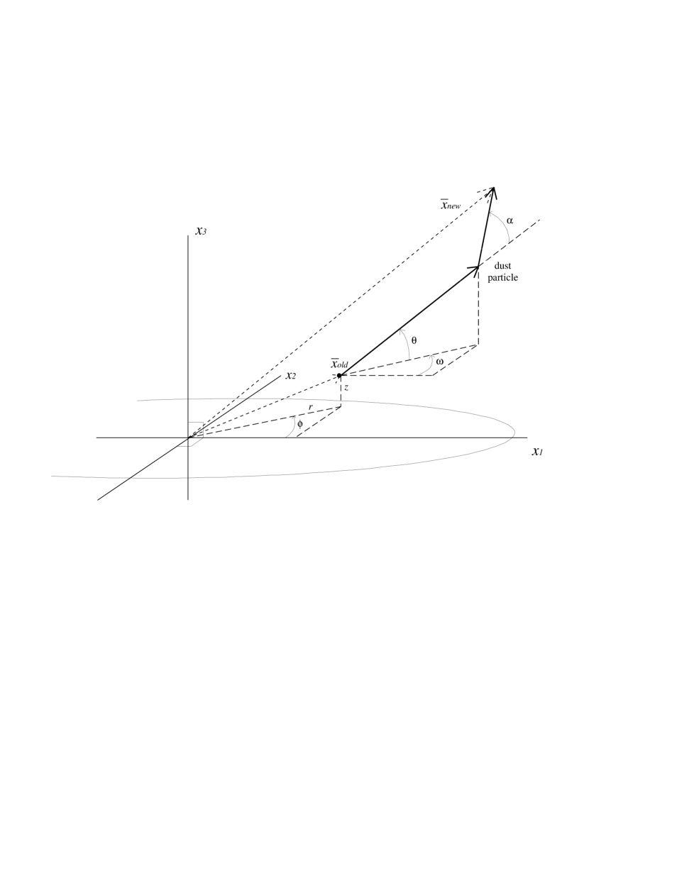
Fig. 12.: The definition of the coordinate system. A trajectory with a scattering is indicated for one step size. A “photon beam” starts at $\overline{x}_{\rm old}$ in the direction defined by ($\omega$,$\theta$), scatters off a dust particle over an angle $\alpha$, and ends at $\overline{x}_{\rm new}$.

A.3 The dust properties

Let us first define the notation for the basic equations of radiative transfer. A beam of light with intensity $I$ is followed while traveling along a straight line through a dusty medium. Since this medium removes a fraction $\kappa\,ds$ of the incident intensity for each distance $ds$ traveled, the full equation is

$$\frac{dI(s)}{ds}=-\kappa(s)I(s)+J(s),$$ (A9)

where $J(s)$ are the new sources of intensity at point $s$ in the travel direction. $\kappa$ is the extinction coefficient and consists of an absorption and a scattering part, and their relative importance is normally expressed by the albedo ($a$)

$$\kappa = \kappa_{a}+\kappa_{s}$$ (A10)

$$a = \kappa_{s}/\kappa.$$ (A11)

While following the light beam through the dusty medium, no new photons were added to the initial beam of photons that was created with intensity $I(0)$, because they are accounted for by the repeating Monte Carlo principle, and $J(s)\!=\!0$. For this single “photon beam” the radiative transfer equation is now

$$\frac{dI(s)}{ds}=-\kappa(s)I(s)$$ (A12)

with formal solution

$$I(x)=I(0){\rm e}^{-\int_{0}^{x}\kappa(s)ds}.$$ (A13)

The integral in Eq.(A13) defines optical thickness

$$\tau\equiv\int_{0}^{x}\kappa(s)\,ds.$$ (A14)

Since the beam was followed while it scattered through the medium (so no longer on a straight line), there were no losses by scattering along the path of the beam. One still can use Eq.(A13), but with $\kappa_{a}(s)\!=\!(1\!-\!a)\kappa(s)$ instead of $\kappa(s)$ as long as the line integral is taken along the path traveled. The extinction coefficient and the albedo are wavelength dependent, which creates reddening of stars and could cause the observed color gradients in the galaxies.

To calculate the absorption along the path traveled, the dust distribution must be defined. The dust extinction coefficient in the models was taken to have a similar distribution as the stellar light, but with a scalelength and scaleheight that were chosen independently:

$$\kappa_{\lambda}(r,z,\phi)=\kappa_{0,\lambda}{\rm e}^{-(r/h_{\rm d}+|z|/z_{\rm d})}$$ (A15)

where $\kappa_{\lambda}(r,z,\phi)$ is the local extinction coefficient at wavelength $\lambda$ and $\kappa_{0,\lambda}$ is the extinction coefficient at $(r\!=\!0,z\!=\!0)$. In this article the optical depth of a system is denoted by the integration of $\kappa_{V}$ ($\kappa$ in the $V$-passband) along the symmetry axis from $(r\!=\!0,z\!=\!-\infty)$ to $(r\!=\!0,z\!=\!\infty)$

$$\tau_{0,V}=\int_{-\infty}^{\ \infty}\kappa_{0,V}{\rm e}^{-|z|/z_{\rm d}}\,dz=2\kappa_{0,V}z_{\rm d}.$$ (A16)

Using Eq.(A13) one can calculate that a point source located behind the center of the galaxy will have suffered an extinction in the $V$-passband for an observer located at its other pole of

$$I(z=\infty)=I(0){\rm e}^{-\tau_{0,V}},$$ (A17)

assuming that all absorbed and scattered photons are lost for a point source.

Three parameters are needed to describe dust properties, the relative extinction $(\tau_{\lambda}/\tau_{V})$, the albedo ($a_{\lambda}$) and the scattering phase function $\Phi_{\lambda}(\alpha)$, and all are dependent on wavelength $(\lambda)$. As there are almost no direct measurements of the dust properties in other galaxies, I decided to use the (also poorly determined) Galactic values. Studies by Knapen et al. ([1991]) and Jansen et al.([1994]) seem to indicate that at least the Galactic extinction curve is applicable to some other galaxies, the other two dust properties have never been measured in extragalactic systems.

For relative extinction, the Galactic extinction properties of Rieke & Lebofsky ([1985]) were used. The values for the albedo were drawn from Bruzual et al.([1988]), as were the values for the scattering asymmetry parameter $g_{\lambda}$. This asymmetry parameter enters in the scattering phase function suggested by Henyey & Greenstein ([1941])

$$\Phi_{\lambda}(\cos(\alpha),g_{\lambda})=[(1-g_{\lambda}^{2})/4\pi](1+g_{\lambda}^{2}-2g_{\lambda}\cos(\alpha))^{-3/2}$$ (A18)

where $\alpha$ is the scattering angle between the incident and the deflected photon. The function is such that $g_{\lambda}\!=\!\langle\cos(\alpha)\rangle$, and thus $-1\!\leq\!g_{\lambda}\!\leq\!1$. Forward scattering dominates for $g_{\lambda}\!>\!0$ and $g_{\lambda}\!=\!0$ results in isotropic scattering. To determine a random deflection angle for a photon with the probability function $\Phi_{\lambda}$ Eq.(A2) can be used and one finds (Witt [1977])

$$\alpha=\arccos(\{(1+g_{\lambda}^{2})-[(1-g_{\lambda}^{2})/(1-g_{\lambda}+2g_{\lambda}R)]^{2}\}/2g_{\lambda}).$$ (A19)

The values used for $\tau_{\lambda}/\tau_{V}$, $a_{\lambda}$, and $g_{\lambda}$ for the different photometric passbands are listed in Table1.

A.4 The numerical method

Each photon beam that was created using Eqs.(A4) and (A6) was stepped through the dusty medium. The step size was determined by the local dust density and was chosen in such way that it would give an optical thickness (absorption plus scattering) of 0.03 if there was a constant dust density along the step. This means that the chance of multiple scattering is of order $(0.03a_{\lambda})^{2}$ along a step. This is negligible, as it should be, because only single scattering was incorporated along each step. It is trivial to show that the step size has to be of order

$$\Delta s=0.03/\kappa(\overline{x})=0.03/(\kappa_{0}{\rm e}^{-(r/h_{\rm s}+|z|/z_{\rm s})})$$ (A20)

and the new position is (if there is no scattering)

$$\overline{x}_{\rm new}=\overline{x}_{\rm old}+\Delta\overline{x}\Delta s.$$ (A21)

For the actual absorption along a step, one has to use Eq.(A13) with $\kappa_{a}\!=\!\kappa(1-a)$ instead of $\kappa$. The integral was at each step approximated by four-point Gauss-Legendre quadrature:

$$\tau_{\Delta s}=\int_{\overline{x}}^{\overline{x}+\Delta\overline{x}\Delta s}\kappa_{a}(\overline{s})\,d\overline{s}\ \ \approx\ \ 0.5\Delta s\sum_{j=1}^{4}w_{j}\,\kappa(\overline{x}+0.5(1+x_{j})\Delta\overline{x})(1-a),$$ (A22)

where the values for $w_{j}$ and $x_{j}$ can be found in any handbook on numerical analysis. When there was no scattering during the step, the $\kappa(\overline{x}_{4})$ calculated in Eq.(A22) was used to determine the step size with Eq.(A20) in the next step.

If scattering did occur, the step proceeded slightly differently. The chance of scattering during a step can be simulated by requiring

$${\rm e}^{-\tau_{\Delta s}a_{\lambda}}<R.$$ (A23)

In that case the directional cosines of Eq.(A7) were changed by an angle given by Eq.(A19). This left another angle of freedom for the azimuthal change of the direction which was generated by

$$\beta=2\pi R.$$ (A24)

Rotating the initial directional angles $\omega,\theta$ over the scattering angles $\alpha,\beta$ gives the new directional cosines

$$\Delta\overline{x}_{\rm new}=\left(\begin{array}[]{rr}\cos(\omega)\cos(\theta)\cos(\beta)&+(\sin(\omega)\cos(\alpha)+\cos(\omega)\sin(\theta)\sin(\alpha))\sin(\beta)\\ \sin(\omega)\cos(\theta)\cos(\beta)&+(-\cos(\omega)\cos(\alpha)+\sin(\omega)\sin(\theta)\sin(\alpha))\sin(\beta)\\ \sin(\theta)\cos(\beta)&-\cos(\theta)\sin(\alpha)\sin(\beta)\\ \end{array}\right).$$ (A25)

When Eq.(A23) was satisfied and scattering occurred in a step, the photon proceeded a fraction $f\!=\!R$ of step size $\Delta s$ in the old direction, before following the new direction

$$\overline{x}_{\rm new}=\overline{x}_{\rm old}+(f\Delta\overline{x}_{\rm old}+(1-f)\Delta\overline{x}_{\rm new})\Delta s.$$ (A26)

A.5 Projection on the sky

The steps in the previous paragraph were repeated until $|\overline{x}_{\rm new}|\!>\!10h_{\rm s}$. All $\tau_{\Delta s}$ of the different steps were added, and the final intensity of the photon beam was $I_{\rm end}\!=\!I_{0}{\rm e}^{-\tau_{\rm tot}}$. The final intensities were projected on the sky as if the galaxy was being observed from infinity. Due to the axisymmetric nature of the models, one can ignore the $\omega$ dependence of the exit direction and rotate all photons over angle $\omega$ as if they leave the galaxy in the same direction. The projection on the $(y_{1},y_{2})$-plane becomes

$$\overline{y}=\left(\begin{array}[]{rrr}-\sin(\omega)&\cos(\omega)&0\\ -\sin(\theta)\cos(\omega)&-\sin(\theta)\sin(\omega)&\cos(\theta)\end{array}\right)\overline{x}$$ (A27)

This procedure of creating photons, stepping through the medium and projecting the exiting photons on the sky was repeated for two million photons. The photons were binned into pixel images in $(y_{1},y_{2})$ direction and the binning in viewing angle $\theta$ direction resulted in ten model images from edge-on to face-on. The binning of photons in the $\theta$ direction was in equal steps of $b/a$, where $b/a$ is the axial ratio of an inclined circle. This has the advantage that each image has approximately equal flux, at least in the case of no extinction. For the analyses discussed in this paper only the face-on images were used, which contained the photons that exited with an angle between 90^∘ and 71.8^∘ (i.e. $1\!\geq\!b/a\!>\!0.95$).

A.6 Testing and the results

The computer program was tested extensively to ensure that the results were reliable. First, a point source emitting all its photons to a pole was placed at the center of the galaxy and the exiting flux was correctly described by Eq.(A17). Tests showed that in the case of no absorption all images at different viewing angle had an equal flux. Tests were made to ensure that the scattering angle phase function was produced correctly and that the angle between the incident and the deflected photon was indeed the required angle. One of the most important tests was the independence of the number of scatterings on step size. If the step size had been too large or if the calculation $\tau_{\Delta s}$ had been incorrect this could not have been the case. The model profiles were tested against the analytic profiles of DDP for the cases with and without scattering. In the case of no scattering (all scattered photons were removed to mimic absorption) the agreement was perfect. Figure5 shows an excellent agreement between the two models even with scattering, as long as the extinction is high. All test results were correct to within the statistical noise.

For the extraction of the (color)profiles, the same programs as in PaperI were used and the model results can be compared directly with the data. Once a $\tau_{0,V}$ and a set of scalelengths and heights have been chosen for a particular model, $\kappa_{0,\lambda}$ is determined by Eq.(A16) and the corresponding optical depths for the other passbands are determined by Table1. This model is also useful to study inclination-dependent effects of extinction.

References

- 1978 Aaronson M. 1978, ApJ 221, L103
- 1992 Andredakis Y.C., van der Kruit P.C. 1992, A&A 265, 396
- 1991 Aoki T.E., Hiromoto N., Takami H., Okamura S. 1991, PASJ 43, 755
- 1944 Baade W. 1944, ApJ 100, 137
- 1987 Begeman K. 1987, Ph.D.Thesis, University of Groningen, The Netherlands
- 1993 Bershady M.A. 1993, PASP 105, 1028
- 1979 Bessell M.S. 1979, PASP 91, 589
- 1994 Block D.L., Witt A.N., Grosbøl P., Stockton A., Moneti A. 1994, A&A 288, 383
- 1978 Bosma A. 1978, Ph.D.Thesis, University of Groningen, The Netherlands
- 1993 Bressan A., Fagotto F., Bertelli G., Chiosi C. 1993, A&AS 100, 647
- 1992 Broeils A. 1992, Ph.D.Thesis, University of Groningen, The Netherlands
- 1993 Bruzual G.A., Charlot S. 1993, ApJ 405, 538
- 1996 Bruzual G.A., Charlot S. 1996, ApJ in preparation (BC96)
- 1988 Bruzual G.A., Magris G.C., Calvet N. 1988, ApJ 333, 673
- 1984 Burstein D., Heiles C. 1984, ApJS 54, 33
- 1989 Buzoni A. 1989, ApJS 71, 817
- 1994 Byun Y.I., Freeman K.C., Kylafis N.D. 1994, ApJ 432, 114
- 1991 Charlot S., Bruzual G.A. 1991, ApJ 367, 126
- 1995 Charlot S., Worthey G., Bressan A. 1995, ApJ submitted
- 1987 Cornell M., E., Aaronson M., Bothun G., Mould J. 1987, ApJS 64, 507
- 1995 de Jong R.S. 1995, Ph.D.Thesis, University of Groningen, The Netherlands
- 1996a de Jong R.S. 1996a, A&A in press (PaperII)
- 1996b de Jong R.S. 1996b, A&A in press (PaperIII)
- 1996c de Jong R.S. 1996c, In: Spiral Galaxies in the near-infrared, eds. D.Minniti, H.-W.Rix (ESO Workshop series), in press
- 1994 de Jong R.S., van der Kruit P.C. 1994, A&AS 106, 451 (PaperI)
- 1991 de Vaucouleurs G., de Vaucouleurs A., Corwin H.G., Buta R.J. et al. 1991, Third Reference Catalog of Bright Galaxies (Springer-Verlag, New York) (RC3)
- 1989 Disney M.J., Davies J.I., Phillipps S. 1989, MNRAS 239, 939 (DDP)
- 1994 Dopita M.A., Ryder S.D. 1994, ApJ 430, 163
- 1994 Evans R. 1994, MNRAS 266, 511
- 1970 Freeman K.C. 1970, ApJ 160, 811
- 1985 Frogel J.A. 1985, ApJ 298, 528
- 1989 Gilmore G., King I., van der Kruit P.C. 1989, The Milky Way as a Galaxy (Geneva Observatory, Sauverny-Versoix, Switzerland)
- 1994 Giovanelli R., Haynes M.P., Salzer J.J., Wegner G., Da Costa L.N., Freudling W. 1994, AJ 107, 2036
- 1994 Goudfrooij P. 1994, Ph.D. Thesis, University of Amsterdam, The Netherlands
- 1994 Goudfrooij P., Hansen L., Jørgensen H.E., Nørgaard-Nielsen H.U., de Jong T., van den Hoek L.B. 1994, A&AS 104, 179
- 1987 Green E.M., Demarque P., King C.R. 1987, The Revised Yale Isochrones and Luminosity Functions (Yale University Observatory, New Haven)
- 1989 Grevesse N., Anders E. 1989, in: Cosmic Abundances of Matter, AIP Conference Proceedings 183, ed. C.J.Waddington (AIP, New York)
- 1992 Han M. 1992, ApJS 81, 35
- 1941 Henyey, L.G., Greenstein, J.L., 1941, ApJ, 93, 70
- 1994 Huizinga J.E. 1994, Ph.D.Thesis, University of Groningen, The Netherlands
- 1994 Jansen R.A., Knapen J.H., Beckman J.E., Peletier R.F., Hes R. 1994, MNRAS 270, 373
- 1996 Just A., Fuchs B., Wielen R. 1996, A&A in press
- 1989 Kennicutt Jr. R.C. 1989, ApJ 344, 685
- 1984 Kent S.M. 1984, ApJS 56, 105
- 1986 Kent S.M. 1986, AJ 91, 1301
- 1987 Kent S.M. 1987, AJ 93, 816
- 1991 Knapen J.H., Hes R., Beckman J.E., Peletier R.F. 1991, A&A 241, 42
- 1987 Kylafis N.D., Bahcall J.N. 1987, ApJ 317, 637
- 1989 Lauberts A., Valentijn E.A. 1989, The Surface Photometry Catalogue of the ESO Sky Survey (ESO, Garching) (ESO-LV)
- 1987 Lin D.N.C., Pringle J.E. 1987, ApJ 320, L87
- 1991 Maeder A., Meynet G. 1991, A&AS 89, 451
- 1992 Mathewson D.S., Ford V.L., Buchhorn M. 1992, ApJS 81, 413
- 1990 Mathis J.S. 1990, ARA&A 28, 37
- 1989 Matteucci F. 1989, in: Evolutionary Phenomena in Galaxies, eds. J.E. Beckman, B.E.J. Pagel (Cambridge University Press, Cambridge), p.297
- 1992 Matteucci F. 1992, in Morphological and Physical Classification of Galaxies, eds. G. Longo, M. Capaccioli, G. Busarello (Kluwer Academic Publishers, Dordrecht), p.245
- 1973 Nilson P. 1973, Uppsala General Catalog of Galaxies (Roy.Soc.Sci., Uppsala) (UGC)
- 1987 O’Connell R.W. 1987, in Stellar Populations, eds. C.Norman, A.Renzini, M.Tosi (Cambridge University press, Cambridge), p.167
- 1989 Peletier R.F. 1989, Ph.D.Thesis, University of Groningen, The Netherlands
- 1990a Peletier R.F., Davies R.L., Davis L.E., Illingworth G.D., Cawson M. 1990a, AJ 100, 1091
- 1994 Peletier R.F., Valentijn E.A., Moorwood A.F.M., Freudling W. 1994, A&AS 108, 621
- 1995 Peletier R.F., Valentijn E.A., Moorwood A.F.M., Freudling W., J.H. Knapen, J.E. Beckman 1995, A&A Letters 300, L1
- 1985 Pickles A.J. 1985, AJ 296, 340
- 1986 Renzini A., Buzzoni A. 1986, in Spectral Evolution of Galaxies, eds. C.Chiosi, A.Renzini (Reidel, Dordrecht)
- 1985 Rieke G.H., Lebofsky M.J. 1985, ApJ 288, 618
- 1993 Rix H.-W., Rieke M.J. 1993, ApJ 418, 123
- 1985 Rubin V.C., Burstein D., Ford Jr. W.K., Thonnard N. 1985, ApJ 289, 81
- 1994 Ryder S.D., Dopita M.A. 1994, ApJ 430, 142
- 1955 Salpeter E.E. 1955, ApJ 121, 161
- 1976 Schweizer F. 1976, ApJS 31, 313
- 1973 Searle L., Sargent W.L.W., Bagnuolo W.G. 1973, ApJ 179, 427
- 1994 Silva D.R., Elston R. 1994, ApJ 428, 511
- 1990 Sommer-Larsen J., Yoshii Y. 1990, MNRAS 243, 468
- 1994 Terndrup D.M., Davies R.L., Frogel, J.A., DePoy D.L., Wells L.A. 1994, ApJ 432, 518
- 1980 Tinsley B.M. 1980, Fund. of Cos. Phys. 5, 287
- 1977 Tully R.B., Fisher J.R. 1977, A&A 54, 661
- 1990 Valentijn E.A. 1990, Nat 346, 153
- 1994 Valentijn E.A. 1994, MNRAS 266, 614
- 1985 van Albada T.S., Bahcall J.N., Begeman K.G., Sancisi R. 1985, ApJ 295, 305
- 1986 van Albada T.S., Sancisi R. 1986, Phil. Trans. (Roy. Soc. London) A320, 447
- 1985 VandenBerg D.A. 1985, ApJS 58, 711
- 1988 van der Kruit P.C. 1988, A&A 192, 117
- 1994 von Alvensleben U.A., Gerhard O.E. 1994, A&A 285, 751
- 1992 Villa-Costas M.B., Edmunds M.G. 1992, MNRAS 259, 121
- 1989 Wainscoat R.J., Freeman K.C., Hyland A.R. 1989, ApJ 337, 163
- 1986 Wevers B.M.H.R., van der Kruit P.C., Allen R.J. 1986, A&AS 66, 505
- 1977 Witt A.N., 1977, ApJS 35, 1
- 1992 Witt A.N., Thronson Jr. H.A., Capuano Jr. J.M. 1992, ApJ 393, 611
- 1994 Worthey G. 1994, ApJS 95, 107 (W94)
- 1988 Wyse R.F.G., Gilmore G 1988, AJ 95, 1404
- 1989 Wyse R.F.G., Silk J. 1989, ApJ 339, 700
- 1994 Zaritsky D., Kennicutt Jr. R.C., Huchra J.P. 1994, ApJ 420, 87