Clumpy ultracompact H II regions – III.
Cometary morphologies around stationary stars

Abstract

Cometary ultracompact H$\,\scriptstyle\rm II$ regions have been modelled as the interaction of the hypersonic wind from a moving star with the molecular cloud which surrounds the star. We here show that a similar morphology can ensue even if the star is stationary with respect to the cloud material. We assume that the H$\,\scriptstyle\rm II$ region is within a stellar wind bubble which is strongly mass loaded: the cometary shape results from a gradient in the distribution of mass loading sources. This model circumvents problems associated with the necessarily high spatial velocities of stars in the moving star models.

1 Introduction

The ultracompact H$\,\scriptstyle\rm II$ regions (UCHiiR) found deep within molecular clouds provide important information on the early phases of the interaction of massive stars with their natal environment. The disruption of the cloud material by the hypersonic winds and UV radiation fields of these stars is a severe barrier to an understanding of the process of massive star formation – only by studying the disruption process will anything be learnt about the innermost regions of the protostellar cloud. The disruption process also involves many important problems of gas dynamics. Considerable theoretical effort has gone into modelling the varied morphology of UCHiiR.

Most theoretical attention has so far been given to the cometary regions, which comprise about 20 per cent of observed UCHiiR [1990]. Perhaps the most detailed model, that of Van Buren & Mac Low (1992, and references therein), treats them as the steady-state partially ionized structures behind bow shocks driven by the winds of stars moving through molecular cloud material. Although it has been argued that some morphologies which are not apparently cometary (in particular, core–halo) can be explained as cometary structures viewed close to their axes [1991], the shell and multiply peaked morphologies cannot, and so other models should also be investigated.

There are also a number of unresolved questions with regard to the cometary models. First, the star is assumed to be moving through relatively homogeneous molecular cloud gas. Yet it is well known that cloud material has a clumpy distribution down to very small scales. Secondly, current cometary models require rather high stellar velocities, characteristically 10–20$\,{\rm{km\,s^{-1}}}$ (Van Buren & Mac Low 1992; Garay, Lizano & Gomez 1994). The origin of such a high velocity dispersion is problematic. Moreover, as emphasized by Gaume, Fey & Claussen [1994], if these high stellar velocities are correct, the vast majority of UCHiiR should be well isolated from other structures for most of their lifetime. Yet they often appear closely associated with other radio continuum sources and molecular cores [1994].

Churchwell [1995] argues that the parameters used by Van Buren & Mac Low [1992] have a fairly large range of possible values. In particular, the ambient density used in these models is significantly smaller than has been observed ahead of some UCHiiR [1994]. Since the shape of the bow shock is determined by the ram pressure of the impinging molecular material, such high densities will allow cometary regions to form for substantially smaller relative velocities. However, such high densities are not common, and are likely to be confined to relatively small clumps. Since these clumps will not be immediately destroyed on their passage through the bow shock, the model discussed in the present paper may in fact be a more appropriate description of the structure of these regions.

Finally, as more detailed observations become available, the similarity of shape to the structures predicted by Van Buren & Mac Low [1992] becomes less convincing. Some of the cometary UCHiiR observed by Gaume et al. [1995] have tails that hook back around the centre of the nebula, while the bow shock model predicts structures with bright arcs and diffuse tails – Gaume et al. indeed propose that such arc-like regions be considered a separate morphological class. When observed at higher resolution, apparently cometary structures often seem to dissolve into collections of individual emission knots (e.g. Kurtz, Churchwell & Wood 1994), rather than remaining as smooth structures.

Dyson [1994] and Lizano & Cantó [1995] have suggested that the interaction of a massive star with clumpy molecular material provides a natural alternative model for UCHiiR, which circumvents the problem of the relatively long ($10^{5}\,{\rm{yr}}$) lifetimes required by their high frequency compared to field OB stars [1990]. Clumps act as localized reservoirs of gas which can be injected into their surroundings by photoionization and/or hydrodynamic ablation. The ionized region is bounded by a recombination front; that is to say, an H$\,\scriptstyle\rm II$ region is held at a constant radius by the high gas density which results from the mass loading. The frictional heating of the flow in mass loading regions may explain the very high temperatures inferred for some fraction of the gas in the Sgr B2 F complex [1995].

There are many possible variants of this basic premise. Dyson, Williams & Redman [Paper I, 1995 – hereafter] have described models in which a strong stellar wind mass loads from clumps. In the model presented in Paper I (as in the present paper), the ionized gas flow is everywhere supersonic. Redman, Williams & Dyson [Paper II, 1996 – hereafter] have discussed models where either the wind is so weak or the mass loading is so great that the interior flow shocks or is totally subsonic.

The models of Papers I and II are spherically symmetric, and reproduce well many observed morphologies (e.g. shell-like and centre-brightened). They cannot, of course, produce cometary morphologies. We here describe how a simple geometrical distribution of mass loading centres can generate such morphologies. This model has two important properties. First, it again exploits the clumpy nature of clouds. Secondly, the star can be at rest with respect to the cloud. The structures predicted are dependent only in detail on the exact form of the mass loading distribution. We consider here only the simplest case, namely where the flow in the UCHiiR remains supersonic, and defer a discussion of the much more complex subsonic flows, and those in which an initially supersonic wind goes through a termination shock, to a later paper.

2 Model

We adapt the supersonic, dust-free, isothermal flow model of Paper I to include a non-spherical distribution of mass loading sources. As in Paper I, we take the stellar wind momentum output rate, ${\dot{\mu}_{\star}}$, as

$${\dot{\mu}_{\star}}=4\pi r^{2}\rho v^{2}={\it const},$$ (1)

where $r$ is the distance from the star, $\rho$ is the gas density and $v$ is the velocity of the flow. In this supersonic model, we assume that the streamlines are essentially radial. Hence, we assume equation (1) holds within any solid angle element and take the mass conservation equation to be

$${1\over r^{2}}\mathchoice{\partial{}\over\partial{r}}{\partial{}/\partial{r}}{\partial{}/\partial{r}}{\partial{}/\partial{r}}\left(r^{2}\rho v\right)=\dot{q}=\dot{q}_{0}\exp(r\cos\theta/\lambda),$$ (2)

where $\dot{q}$ is the mass loading rate and $\lambda$ is the scale height of the mass loading distribution. In this model, $\rho$ and $v$ are thus functions both of the distance from the central ionizing source, $r$, and of the azimuthal angle, $\theta$.

The distribution of mass loading has been chosen to vary as a function of the distance, $x=r\cos\theta$, perpendicular to a certain plane through the star (this is not the conventional correspondence, as the Cartesian co-ordinates are oriented by the line of sight assumed to the region, while the spherical polars are oriented by its symmetry axis). At large positive $x$, the mass loading is great, whereas it decreases to a negligible level at large negative $x$. Such a distribution of mass loading might be expected where a young ionizing star formed at the border of a molecular cloud. Closer in to the centre of the cloud, an increased density of mass loading clumps will produce a higher mean mass loading rate; away from the cloud, the mean density of material will decrease and the mass loading rate will drop.

Integrating equation (2), we find that, once the mass flux is dominated by the mass loading material, the flow density is

$$\rho={4\pi\over{\dot{\mu}_{\star}}}{\dot{q}_{0}^{2}\lambda^{4}\over\cos^{4}\theta}{1\over\tau^{2}}\left[\left(\tau^{2}-2\tau+2\right)\exp(\tau)-2\right]^{2},$$ (3)

where $\tau=r\cos\theta/\lambda$. The recombination front radius, $R_{\rm R}$ (which is a function of the angle, $\theta$), follows from the Strömgren relationship in a solid angle element d$\Omega$:

$$\int_{0}^{R_{\rm R}}\beta n^{2}r^{2}{\rm\,d}{r}{\rm\,d}{\Omega}=S_{\star}\left({\rm d}\Omega\over 4\pi\right),$$ (4)

where $\beta$ is the case B recombination coefficient, $n=\rho/\bar{m}$ is the number density of nucleons (we assume the gas inside the recombination front is almost completely ionized), and $S_{\star}$ is the total stellar output of Lyman continuum photons. Hence

$$\cos\theta = \lambda\left(64\pi^{3}\beta\dot{q}_{0}^{4}\over S_{\star}{\dot{\mu}_{\star}}^{2}\bar{m}^{2}\right)^{1/11}I(\tau_{\rm R})^{1/11}$$ (5)

$$= \left(\lambda\over 8{\times 10^{16}}\,{\rm{cm}}\right)\dot{q}_{-30}^{4/11}S_{48}^{-1/11}\dot{\mu}_{28}^{-2/11}I(\tau_{\rm R})^{1/11},$$ (6)

where $\tau_{\rm R}=R_{\rm R}\cos\theta/\lambda$ and

$$I(\tau)\equiv\int_{0}^{\tau}\left[\left(\tau^{2}-2\tau+2\right)\exp(\tau)-2\right]^{4}{{\rm\,d}\tau\over\tau^{2}}.$$ (7)

In equation (6), we have taken $\beta=2{\times 10^{-13}}\,{\rm{cm}}^{3}\,{\rm{s}}^{-1}$, $\bar{m}=2{\times 10^{-24}}\,{\rm{g}}$, and defined scaling variables $S_{48}\equiv S_{\star}/10^{48}\,{\rm{s}}^{-1}$, $\dot{\mu}_{28}\equiv{\dot{\mu}_{\star}}/10^{28}\,{\rm{g}}\,{\rm{cm}}\,{\rm{s}}^{-2}$ and $\dot{q}_{-30}\equiv\dot{q}/10^{-30}\,{\rm{g}}\,{\rm{cm}}^{-3}\,{\rm{s}}^{-1}$ (cf. Paper I).

Figure 1: The function $I(\tau)^{1/11}$, which determines the shape of the cometary regions (cf. equation (5)).

Figure 2: Cometary shapes, for a range of UCHiiR sizes relative to the scale height of the mass loading distribution. The star is, in all cases, at the intersection of the axes.

(a)	(b)

Figure 3: Grey-scale plot of emission from UCHiiR with non-uniform mass loading, with the recombination front in the direction of least loading ($\theta=\pi$) at (a) $\tau_{\rm tail}=-0.3$, (b) $\tau_{\rm tail}=-1$. The star is at the intersection of the axes. Contours are also shown, at 2.5, 5, 7.5, 10, 20, 30, 40, 50, 60, 70, 80 and 90 per cent of the peak intensity [the faintest contour away from the edge of (a) is at 50 per cent, in (b) at 30 per cent].

Figure 4: Grey-scale and contour emission measure image of a cometary model, for $\tau=-5$ in the ‘tail’. The contours are chosen as in Fig. 3. To the right, line profiles are shown, calculated at the various labelled points. The thin curves are the zero-broadening line profiles, while the bold curves are shown for thermal broadening appropriate to a radial Mach number of 2.2 at the recombination front at the head of the cometary shape. The velocity scale is constant between the profiles, but the peak intensity scale is arbitrary – the total strength of the emission for each observation may be judged from the emission measure value at that point.

In Fig. 1, we plot $I(\tau)^{1/11}$ as a function of $\tau$. From equation (5), the recombination front directly into and against the mass loading gradient occurs where $I(\tau)=\pm{\it const}$: this will be symmetric if $\tau_{\rm R}\ll 1$, but, as $\tau_{\rm R}$ increases, the ionized region will soon become highly asymmetric. The tail of the curve at large negative $\tau$ tends to a constant value of $I(\tau)$: for high enough ionizing fluxes, the flow in the direction of low mass loading is essentially free and the gas remains ionized at all radii (within the assumptions of this model).

In Fig. 2, we plot the loci of $R_{\rm R}(\theta)$ (i.e. the envelopes of the UCHiiR when seen from a direction perpendicular to the density gradient), for a range of UCHiiR sizes relative to the exponential scale height – these curves are given parametrically by equation (5).

2.1 Emission measure

In this paper, we consider only the simplest case of cometary structures observed edge-on. We define Cartesian coordinates $(x,y,z)$ with the star at the origin, where $(x,y)$ are in the plane of the sky and $x=r\cos\theta$. The emission measure at $x=b_{1}$, $y=b_{2}$ is given by the integral along the line of sight (parallel to $z$)

$${\cal E}(b_{1},b_{2}) = \int n^{2}{\rm\,d}{z}$$ (9)

$$= \dot{q}_{0}^{4}\left(4\pi\over{\dot{\mu}_{\star}}\bar{m}\right)^{2}\left[(\tau^{2}-2\tau+2)\exp(\tau)-2\over\tau^{3}\right]^{4}$$

$$\quad\times\int_{-z_{\rm R}}^{z_{\rm R}}r^{8}{\rm\,d}{z},$$

where $\tau=b_{1}/\lambda$ and $z_{\rm R}$ is given by $z_{\rm R}^{2}=b_{1}^{2}\tan^{2}\theta_{\rm R}-b_{2}^{2}$, with $\theta_{\rm R}$ given by equation (5).

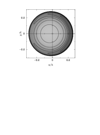
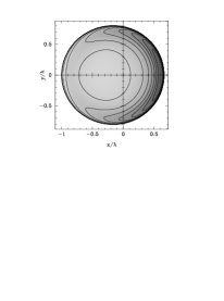
Example plots of the emission measure are shown in Figs 3 and 4, with contours chosen to be similar to those used in observational papers. The size of the cometary structures is parametrized by $\tau_{\rm tail}$, the value of $\tau_{\rm R}$ in the direction of the tail, $\theta=\pi$. The two cases shown in Fig. 3 demonstrate the appearance of the cometary form as the size of the UCHiiR increases relative to the scale of the non-uniformity in mass loading. For $\tau_{\rm tail}=-0.3$, the region is mildly aspherical and may be compared to the models of Paper I. For $\tau_{\rm tail}=-1$, the structure is similar to that of the arc-like UCHiiR described by Gaume et al. [1995]. When $\tau_{\rm tail}=-5$, the morphology is cometary.

2.2 Line profiles

Optically thin line profiles can be calculated from the equation

$${\cal E}(b_{1},b_{2},v_{\rm l})=\int_{-z_{\rm R}}^{z_{\rm R}}n^{2}f\left({z\over r}v_{r}-v_{\rm l}\right){\rm\,d}{z},$$ (10)

where $(b_{1},b_{2})$ are the coordinates $(x,y)$ of the point observed in the nebula, and the line-of-sight component of the velocity is $v_{\rm l}$. The distance $r$ is given, as above, as a function of $z$. The flow velocity, $v_{r}(b_{1},b_{2},z)$, is given by equations (1) and (3) as

$$v_{r}={1\over r^{3}}{{\dot{\mu}_{\star}}\over 4\pi\dot{q}_{0}}\left[b_{1}^{3}\over(b_{1}^{2}-2b_{1}+2)\exp(b_{1})-2\right],$$ (11)

i.e., $v_{r}=A(b_{1})/r^{3}$, where $A(b_{1})$ is a constant for each line of sight.

In the limit of zero broadening (where $f(v)=\delta(v)$, the Kronecker delta function), contributions to the integral, equation (10), come at solutions, $z_{i}$, of the quartic equation

$$(b^{2}+z_{i}^{2})^{2}v_{\rm l}=z_{i}A(b_{1}),$$ (12)

in the range $[-z_{\rm R},z_{\rm R}]$, where $b^{2}=b_{1}^{2}+b_{2}^{2}$. The line profile is then given by

$${\cal E}(b_{1},b_{2},v_{\rm l})=\sum_{\{z_{i}\}}\left[n(b_{1},b_{2},z_{i})\right]^{2}{(b^{2}+z_{i}^{2})^{3}\over A(b_{1})\char 124\relax b^{2}-3z_{i}^{2}\char 124\relax}.$$ (13)

Line profiles including broadening can be obtained by convolving this line profile by a line-of-sight velocity function $g(v)$. This integration will remove the singularity in equation (13) where $z_{i}^{2}=b^{2}/3$. For instance, thermal broadening is given by convolving with a Gaussian

$$g(v)={1\over\sqrt{2\pi}\sigma}\exp(-v^{2}/2\sigma^{2}),$$ (14)

where the one-dimensional velocity dispersion, $\sigma$, is given by $\sigma^{2}=k_{\rm B}T/M_{\rm Z}=\bar{m}c^{2}/M_{\rm Z}$ for line emission from a species of atomic mass $M_{\rm Z}$, if $\bar{m}$ is the mean mass per particle and $c$ is the isothermal sound speed. If the integral, equation (10), is performed directly with $f(v)=g(v)$ given by equation (14), major contributions to the total will come from near the solutions $z_{i}$ of equation (12) and from line-of-sight velocity extrema.

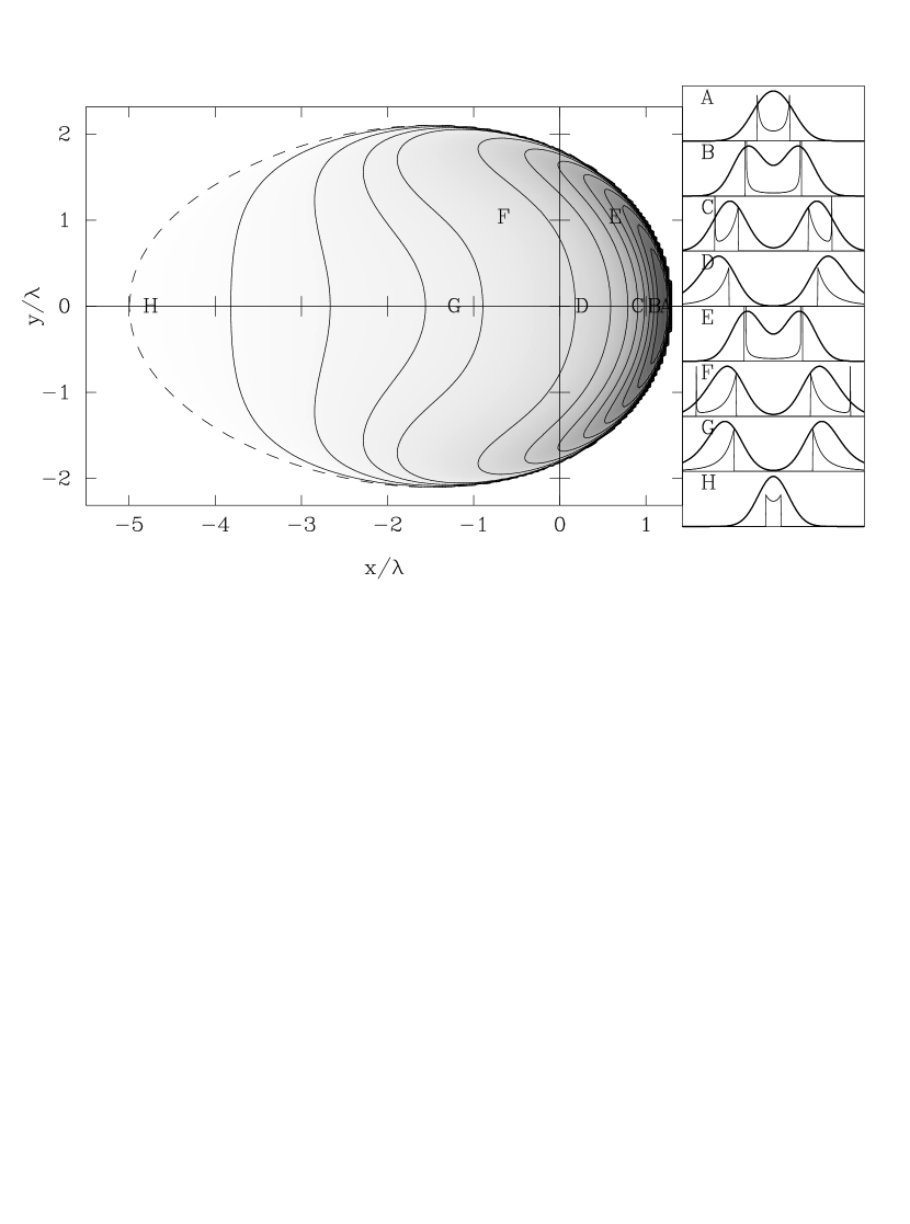
In Fig. 4, we present line profiles for a selection of points within the cometary shape. Close to the edge of the region (points A, H), the flow is nearly in the plane of the sky, and the line widths are only slightly above the thermal widths. For lines of sight further into the nebula (points B, C, D), a larger component of the flow velocity will be seen: the line profiles become increasingly double-peaked. Further around the bright shell (point E), the double-peaked profiles are similar to those found along a line to the apex. The unbroadened profiles at points C and F show the sharp peak at the maximum line-of-sight flow velocity, but when smoothed by the thermal broadening this has little obvious effect. At points D and G, this spike is outside the range of velocities displayed in Fig. 4: the line profile has two fairly well-separated components, with noticeably stronger tails to high velocity.

Figure 5: Channel maps for cometary UCHiiR, shown for velocities $v$ as fractions of the radial velocity at the recombination front, $v_{r,\rm h}$, at the head of the comet ($\theta=0$). The profiles are thermally broadened assuming that this velocity is $22\,{\rm{km\,s^{-1}}}$, i.e. Mach 2.2. The grey-scale representation is normalized in each image; the contours are scaled to 2.5, 5, 7.5, 10, 20, 30, 40, 50, 60, 70, 80 and 90 per cent of the peak intensity in the $v=0$ channel map. The ticks on the axis are at intervals of $\lambda$, the scale height of the mass loading distribution; the dashed contour at the edge of the region is as in Fig. 4.

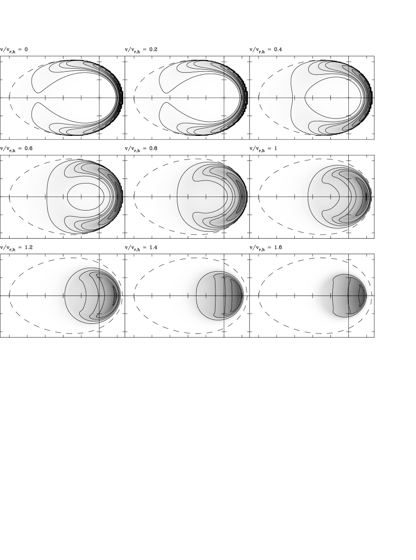
In Fig. 5, we present the line profile data in the form of maps at a single velocity (similar to observational ‘channel maps’). These are shown for single velocities, $v$, but, since the emission has been thermally broadened, they show the structures expected for narrow-bandpass observations. At low velocities, the emission is bright, and is dominated by the dense gas at the edge of the UCHiiR. As the relative velocity of the bandpass increases, however, the emission peak gradually draws away from the edge of the region and fills in the central hollow.

This displacement of the peak of the diffuse emission with increasing relative velocity is a characteristic of radial flow models such as that discussed here. In contrast, in the bow shock and ‘champagne’ models, significant line-of-sight velocities can be produced at the edge of the region by flows around the shell structure. The finite spatial resolution of radio observations and the presence of strong, discrete emission components will, however, confuse this as an observational diagnostic. As can be seen from Fig. 5, the emission will only begin to become centre-brightened at relative velocities $\ga 22\,{\rm{km\,s^{-1}}}$, and with emission intensities $\la 10$ per cent of the peak in the zero-velocity image.

These conclusions are, however, strongly dependent on the model assumption that the dominant mechanism which broadens the emission is thermal broadening. As we argued in Paper I, the emission from supersonic mass loaded winds is likely to be dominated by the dense gas near to individual clumps. The effect of the finite number of individual clumps will be more noticeable in velocity-resolved observations of UCHiiR. Also, the tails are likely to be very dynamically active, with characteristic turbulent velocities similar to the shear velocity between the wind flow and the (small) clump velocity. A dependence of this type would serve to fill in, at least in part, the faint central regions of the low-velocity maps. Firm conclusions must, therefore, await a detailed treatment of the line emission from the regions around individual mass loading clumps, which is beyond the scope of this paper.

3 Conclusions

In this paper, we have shown how cometary morphologies may readily be produced in a mass loaded model for UCHiiR, with no need for relative motion between the central young OB star and the molecular cloud material, if mass loading sources are concentrated to one side. Velocity channel maps show a shell structure stronger than the integrated emission at small velocities relative to systemic, becoming centre-brightened at higher relative velocities. We have assumed that the lines are broadened only to the thermal width: in reality, however, the velocity structure may be dominated by turbulence in the dense gas around individual mass loading sources.

We have assumed an exponential distribution in the rate of mass loading with distance, $x$, away from a plane containing the star. The general shape of the regions is not strongly dependent on the detailed form of the mass loading distribution, so long as it has a general decrease in one direction. In one direction, the recombination front is trapped close to the star by a high rate of mass loading, while in the opposing direction the material remains ionized to a rather larger radius, or even out to infinity. Such distributions might result not only near the edge of a molecular core, but also if a small relative motion carried clumps into the UCHiiR which were then evaporated as they crossed it.

Related models can be considered for different distributions of mass loading centres: for instance, if the luminous star formed on a ridge of clumpy molecular material (or surrounded by a thick disc), the resultant UCHiiR would have a bipolar morphology. This can be pictured by imagining a mirror placed at the plane $x=0$ of Fig. 4, to produce a structure of two back-to-back cometary tails.

The model discussed here will give rise to observable velocity gradients in the head-to-tail direction when the symmetry axis is inclined to the plane of the sky. Since the velocity of gas crossing the recombination front, $v_{\rm R}$, is nearly constant around the comet (to within 50 per cent even when the tail is 50 scale lengths away from the star), the maximum observed difference in mean line-of-sight velocity will be $\sim 2v_{\rm R}\sin i$, for inclination angle $i$. Garay et al. [1994] find differences of $8$–$12\,{\rm{km\,s^{-1}}}$ between the mean velocities of emission in the head and tail of three cometary UCHiiR, which can be fitted with a mild inclination of the cometary axis to the plane of the sky.

While Garay et al. [1994] find no velocity gradients across the regions they observe, Gaume et al. [1994] list three well-defined cometary regions which have an asymmetric velocity gradient perpendicular to the continuum symmetry axis of the UCHiiR. This observation is problematic for the model discussed here, as it is also for the bow shock model. These contradictory results may relate to morphology: Gaume et al.’s sample tend to have significantly longer and more complex tails, while Garay et al.’s sample are more arc-like.

We find that such arc-like morphologies are produced for milder asymmetries in mass loading. They form a natural intermediate between shell and cometary morphologies. Indeed, we would expect arc-like morphologies also to be found in bow shock models for UCHiiR, if the relative velocity of cloud and star were low: such a model might, however, have too low a gas pressure to correspond to observed UCHiiR.

Kurtz et al. [1994] find some observational evidence for a size–density relationship for spherical and unresolved regions, but not for cometary and core–halo UCHiiR. This suggests that a Strömgren relation might hold for the former class, but not for the latter. However, given the sparse data on which these correlations are based (which do not allow, for instance, for correction for the luminosity function of the stars), we do not view this as a conclusive argument against the model discussed in the current paper.

In subsequent papers, we will address the effects of tangential pressure forces in mildly supersonic models and the structures expected when the anisotropic mass loading is sufficiently strong to produce a subsonic region of the flow.

References

- [1994] Cesaroni R., Churchwell E.B., Hofner P., Walmsley C.M., Kurtz S., 1994, A&A, 288, 903?
- [1990] Churchwell E.B., 1990, A&AR, 2, 79
- [1995] Churchwell E.B., 1995, Ap&SS, 224, 157
- [1994] Dyson J.E., 1994, in Ray T.P., Beckwith S.V., eds, Lecture Notes in Physics 431: Star Formation Techniques in Infrared and mm-wave Astronomy. Springer-Verlag, Berlin, p. 93
- [Paper I] Dyson J.E., Williams R.J.R., Redman M.P., 1995, MNRAS, 277, 700 (Paper I)
- [1994] Garay G., Lizano S., Gomez Y., 1994, ApJ, 429, 268
- [1994] Gaume R.A., Fey A.L., Claussen M.J., 1994, ApJ, 432, 648
- [1995] Gaume R.A., Claussen M.J., De Pree C.G., Goss W.M., Mehringer D.M., 1995, ApJ, 449, 663
- [1994] Kurtz S., Churchwell E., Wood D.O.S., 1994, ApJS, 91, 659
- [1995] Lizano S., Cantó J., 1995, in Lizano S., Torrelles J.M., eds, Circumstellar Disks, Outflows and Star Formation. Rev. Mex. Astron. Astrofis., Ser. Conf., 1, 29
- [1991] Mac Low M.-M., Van Buren D., Wood D.O.S., Churchwell E., 1991, ApJ, 369, 395
- [1995] Mehringer D.M., De Pree C.G., Gaume R.A., Goss W.M., Claussen M.J., 1995, ApJ, 442, L29
- [Paper II] Redman M.P., Williams R.J.R., Dyson J.E., 1996, in press (Paper II, this issue)
- [1992] Van Buren D., Mac Low M.-M., 1992, ApJ, 394, 534