December 1995 (Final version March 1996) Preprint MPI-PTh 95-120 To be published in Physical Review D E-Print ASTRO-PH/9601111

Neutrino Oscillations and the Supernova 1987A Signal

Abstract

We study the impact of neutrino oscillations on the interpretation of the supernova (SN) 1987A neutrino signal by means of a maximum-likelihood analysis. We focus on oscillations between $\overline{\nu}_{e}$ with $\overline{\nu}_{\mu}$ or $\overline{\nu}_{\tau}$ with those mixing parameters that would solve the solar neutrino problem. For the small-angle MSW solution ($\Delta m^{2}\approx 10^{-5}\,\rm eV^{2}$, $\sin^{2}2\Theta_{0}\approx 0.007$), there are no significant oscillation effects on the Kelvin-Helmholtz cooling signal; we confirm previous best-fit values for the neutron-star binding energy and average spectral $\overline{\nu}_{e}$ temperature. There is only marginal overlap between the upper end of the 95.4% CL inferred range of $\langle E_{\overline{\nu}_{e}}\rangle$ and the lower end of the range of theoretical predictions. Any admixture of the stiffer $\overline{\nu}_{\mu}$ spectrum by oscillations aggravates the conflict between experimentally inferred and theoretically predicted spectral properties. For mixing parameters in the neighborhood of the large-angle MSW solution ($\Delta m^{2}\approx 10^{-5}\,\rm eV^{2}$, $\sin^{2}2\Theta_{0}\approx 0.7$) the oscillations in the SN are adiabatic, but one needs to include the regeneration effect in the Earth which causes the Kamiokande and IMB detectors to observe different $\overline{\nu}_{e}$ spectra. For the solar vacuum solution ($\Delta m^{2}\approx 10^{-10}\,\rm eV^{2}$, $\sin^{2}2\Theta_{0}\approx 1$) the oscillations in the SN are nonadiabatic; vacuum oscillations take place between the SN and the detector. If either of the large-angle solutions were borne out by the upcoming round of solar neutrino experiments, one would have to conclude that the SN 1987A $\overline{\nu}_{\mu}$ and/or $\overline{\nu}_{e}$ spectra had been much softer than predicted by current treatments of neutrino transport.

]

I Introduction

Neutrino oscillations can modify the characteristics of the neutrino signal from a supernova (SN), in particular if matter effects are included [1]. After the observation of the SN 1987A neutrinos by the Kamiokande [2] and IMB [3] detectors many authors [4] discussed the impact of matter-induced oscillations on the prompt $\nu_{e}$ burst because the first event at Kamiokande had been observed in the forward direction, allowing for an interpretation in terms of $\nu_{e}$-$e$ scattering. If this interpretation were correct one could exclude a large area of mixing parameters where the MSW effect in the SN envelope would have rendered the prompt $\nu_{e}$ burst unobservable.

Because a single event does not carry much statistically significant information (the first Kamiokande event may have coincidentally pointed in the forward direction), a more interesting question for the interpretation of the SN 1987A neutrino signal is the impact of oscillations on the main $\overline{\nu}_{e}$ pulse which is detected by the reaction $\overline{\nu}_{e}p\to ne^{+}$. The SN emits roughly equal amounts of energy in (anti)neutrinos of all flavors, but with different spectral characteristics. Current treatments of neutrino transport yield [6]

$$\langle E_{\nu}\rangle=\cases{10{-}12\,{\rm MeV}&for $\nu_{e}$,\cr 14{-}17\,{\rm MeV}&for $\overline{\nu}_{e}$,\cr 24{-}27\,{\rm MeV}&for $\nu_{\mu,\tau}$ and $\overline{\nu}_{\mu,\tau}$,}$$ (1)

i.e. $\langle E_{\nu_{e}}\rangle\approx\frac{2}{3}\langle E_{\overline{\nu}_{e}}\rangle$ and $\langle E_{\nu}\rangle\approx\frac{5}{3}\langle E_{\overline{\nu}_{e}}\rangle$ for the other flavors. A partial conversion between, say, $\overline{\nu}_{\mu}$’s and $\overline{\nu}_{e}$’s due to oscillations would “stiffen” the $\overline{\nu}_{e}$ spectrum observable at Earth [8, 9]. (We will always take $\overline{\nu}_{e}$-$\overline{\nu}_{\mu}$ oscillations to represent either $\overline{\nu}_{e}$-$\overline{\nu}_{\mu}$ or $\overline{\nu}_{e}$-$\overline{\nu}_{\tau}$ oscillations.) Within a plausible range of progenitor star masses and depending on the equation of state, numerical computations yield

$$E_{\rm b}=1.5{-}4.5\times 10^{53}\,{\rm erg}$$ (2)

for the total amount of binding energy [7]. It is almost entirely released in the form of neutrinos.

The expected average SN 1987A $\overline{\nu}_{e}$ energy implied by the detected signal is about $9{-}10\,\rm MeV$, with a 95.4% confidence interval reaching up to $14\,\rm MeV$ in some analyses [10, 11], i.e. barely up to the lower end of the theoretical predictions quoted in Eq. (1). If a partial swap $\overline{\nu}_{e}\leftrightarrow\overline{\nu}_{\mu}$ had occurred, the expected $\overline{\nu}_{e}$ energies should have been lower, causing an even larger strain between measured and predicted $\overline{\nu}_{e}$ energies. For an “inverted” mass matrix with $m_{\nu_{e}}>m_{\nu_{\mu}}$ the $\overline{\nu}_{e}$-$\overline{\nu}_{\mu}$ oscillations would have been resonant and thus nearly complete for a large range of mixing parameters. Therefore, such inverted-mass schemes are likely excluded on the basis of the SN 1987A data [9, 12].

If the mass hierarchy is “normal” with $m_{\nu_{e}}<m_{\nu_{\mu}}$, oscillations in the antineutrino sector are significant only for large mixing angles which are often thought to be unlikely. Therefore, in the original analyses of the SN 1987A neutrinos, little attention has been paid to antineutrino oscillations.

Since then much progress has been made with the observation of solar neutrinos in four experiments which all report a deficit and thus point to oscillations. While it remains uncertain if the solar neutrino deficits are indeed caused by oscillations, it has become clear that there is no simple “astrophysical solution.” If the oscillation interpretation is adopted there remain three islands in the $\sin^{2}2\Theta_{0}$-$\Delta m^{2}$-plane (vacuum mixing angle $\Theta_{0}$) where the results from all experimental measurements of the solar neutrino flux are consistently explained, namely the “vacuum solution” with $\Delta m^{2}$ near $10^{-10}\,\rm eV^{2}$ and nearly maximum mixing [13], the “small-angle MSW solution” with $\Delta m^{2}$ around $10^{-5}\,\rm eV^{2}$ and $\sin^{2}2\Theta_{0}\approx 0.007$, and the “large-angle MSW solution” with about the same $\Delta m^{2}$ and $\sin^{2}2\Theta_{0}$ in the neighborhood of $0.7$ [5]. It will turn out that if one of the large-angle solutions would be borne out by one of the forthcoming experiments Superkamiokande, SNO, or BOREXINO, then a significant impact on the interpretation of the SN 1987A signal could not be avoided.

In a recent study, Smirnov, Spergel, and Bahcall [9] found that the large-angle solutions were essentially excluded by the SN 1987A data because of the “stiffened” spectra they would have caused at the detectors. However, this conclusion relies heavily on theoretical predictions for the spectral properties of a SN neutrino signal. Kernan and Krauss [14], on the other hand, arrive at the opposite conclusion, namely that a significant oscillation effect was actually favored by the data. Of course, they discard certain theoretical predictions for the signal characteristics. Smirnov, Spergel, and Bahcall have performed a joint analysis for the Kamiokande and IMB detectors. However, in the neighborhood of the large-angle MSW solution, matter-induced oscillations in the Earth are important. They cause a different amount of “regeneration” of the oscillations on the neutrino path through the Earth which was 3900 and $8400\,\rm km$ for the Kamiokande and IMB detectors, respectively, which thus would have observed different $\overline{\nu}_{e}$ spectra [15]. Kernan and Krauss, on the other hand, have only considered nonadiabatic oscillations which restrict the validity of their analysis to $\Delta m^{2}\lesssim 10^{-10}\,\rm eV^{2}$, thus ignoring the important case of the large-angle MSW solution.

Therefore, we presently reexamine the impact of large-angle neutrino oscillations on the SN 1987A signal interpretation. If neutrino oscillations between $\overline{\nu}_{e}$ and another flavor occur at all with a large mixing angle, the mixing parameters probably correspond to those solving the solar neutrino problem. Therefore, we focus on mixing parameters in the neighborhood of the large-angle MSW solution and of the vacuum solution of the solar neutrino problem. We will assume thermal neutrino spectra with different temperatures for the $\overline{\nu}_{\mu}$’s and $\overline{\nu}_{e}$’s. We will then perform a maximum-likelihood analysis for the neutrino temperature and total emitted energy.

In Sect. II we discuss the assumed primary neutrino spectra and their modification by oscillations. Sect. III is devoted to our statistical methodology and Sect. IV to detailed numerical results. In Sect. V we summarize our findings.

II Neutrino Spectra

A Primary Spectra

The most detailed statistical analysis of the SN 1987A neutrino signal has been performed in the papers by Loredo and Lamb [10, 11] where one of the main goals was to estimate the Kelvin-Helmholtz cooling time scale of the newly formed neutron star, and to derive limits on the $\overline{\nu}_{e}$ mass from the absence of pulse dispersion effects. Therefore, the time structure of the neutrino signal was crucial; it had to be parametrized in terms of a variety of cooling models. In our study, on the other hand, we will focus on the spectral characteristics of the neutrino fluence (time-integrated flux) and their modification by oscillations. Because we will need to vary neutrino mass differences and mixing angles, the overall number of parameters would get out of hand if we were to analyse the time structure of the burst together with neutrino oscillation effects.

Numerical simulations [17] and an analytic argument [19] indicate an approximate equipartition of the energy emitted in different (anti)neutrino species with different time-averaged energies as quoted in Eq. (1). The detailed spectral shape, however, is not well known. Monte-Carlo studies of neutrino transport [16] indicate that the instantaneous neutrino spectra are “pinched,” meaning that their low- and high-energy parts are suppressed relative to a Maxwell-Boltzmann spectrum of the same average energy. Usually the instantaneous spectra are expressed in the form [16]

$$f(E,t)\propto\frac{E^{2}}{e^{E/T-\eta}+1}\,,$$ (3)

where $\eta$ is an effective degeneracy parameter. Both $T$ and $\eta$ are functions of time. It must be stressed that the “pseudo degeneracy parameter” $\eta$ for $\nu_{\mu}$ and $\nu_{\tau}$ is the same as that for $\overline{\nu}_{\mu}$ and $\overline{\nu}_{\tau}$, in contrast with the degeneracy parameter of a real Fermi-Dirac distribution which has the opposite sign for antineutrinos relative to neutrinos. Therefore, Eq. (3) is a somewhat arbitrary two-parameter representation of the neutrino spectra which allows one to fit two of their moments, for example $\langle E\rangle$ and $\langle E^{2}\rangle$. Janka and Hillebrandt [16] found that throughout the emission process $\eta$ decreases from about 5 to 3 for $\nu_{e}$, from about 2.5 to 2 for $\overline{\nu}_{e}$, and from about 2 to 0 for $\nu_{\mu,\tau}$ and $\overline{\nu}_{\mu,\tau}$.

The time-integrated spectrum, however, need not be pinched. We characterize it by the moments $\langle E\rangle$ and $\langle E^{2}\rangle$, and call it “pinched” if the ratio $\langle E^{2}\rangle/\langle E\rangle^{2}$ is smaller than for the Maxwell-Boltzmann case, “antipinched” otherwise. As a simple example we consider a cooling model where neutrinos are emitted from a neutrino sphere with a fixed radius and an exponentially decreasing effective temperature. If the instantaneous spectra are of the form Eq. (3) with a fixed $\eta$, then the time-integrated spectrum is pinched for $\eta\gtrsim 1.7$ and antipinched for $\eta\lesssim 1.7$. For $\eta\approx 1.7$ it is approximately of the Maxwell-Boltzmann form.

An exponential cooling model is, of course, very simplistic. In a real SN the $\overline{\nu}_{e}$ temperature will initially rise, and may stay approximately constant for some time, while the effectively radiating surface shrinks quickly within the first second. Still, the exponential cooling example illustrates that a thermal Maxwell-Boltzmann spectrum may be a relatively good approximation for the time-integrated spectrum because of the compensating effects between instantaneous pinching and the superposition of different spectra in the course of the protoneutron star’s cooling history. Certainly, there is no reason to expect the time-integrated spectrum to be of the form Eq. (3). This parametrization does not allow one to describe antipinched spectra, only pinched ones.

For the rest of this study we will make the simplifying assumption that the time-integrated spectra are described by the Maxwell-Boltzmann form

$$F(E)=\int_{0}^{\infty}dt\,f(E,t)\propto E^{2}\,e^{-E/T}$$ (4)

with a different effective temperature for $\overline{\nu}_{e}$ and $\overline{\nu}_{\mu}$. These “temperatures” are parameters which characterize the time-integrated spectra by virtue of $T\equiv\frac{1}{3}\langle E\rangle$ and thus do not exactly correspond to a physical temperature at the neutron star.

B Modification by Oscillations

In the Kamiokande and IMB detectors, SN neutrinos are almost exclusively detected by the reaction $\overline{\nu}_{e}p\to ne^{+}$ where the final-state positron is measured by its Cherenkov emission of photons. If neutrinos do not mix, their fluence $F_{\overline{\nu}_{e}}(E)$ relevant for the detection process is identical with the pimary $\overline{\nu}_{e}$ spectrum $F_{\overline{\nu}_{e}}^{0}(E)$ emitted from the SN. In the presence of $\overline{\nu}_{e}\leftrightarrow\overline{\nu}_{\mu}$ oscillations, on the other hand, each primary $\overline{\nu}_{\mu}$ arrives with a probability $p$ in the $\overline{\nu}_{e}$ flavor state at the detector, while each primary $\overline{\nu}_{e}$ arrives as $\overline{\nu}_{e}$ with the “survival probability” $1-p$ so that

$$F_{\overline{\nu}_{e}}=(1-p)\,F_{\overline{\nu}_{e}}^{0}+p\,F_{\overline{\nu}_{\mu}}^{0}.$$ (5)

This incoherent superposition of the individual flavor fluxes is justified by the incoherent neutrino emission from different regions in the star and by different processes [9].

The “permutation factor” $p$ is in general a function of the neutrino energy $E$, the mass difference $\Delta m^{2}$, and the vacuum mixing angle $\Theta_{0}$. In addition, it is important to note that the neutrinos are produced in a region of high matter density. The effective mixing angle in a medium is given by the well-known formula

$$\tan 2\Theta=\frac{\sin 2\Theta_{0}}{\cos 2\Theta_{0}\mp\rho/\rho_{\rm res}}\,,$$ (6)

where $\Theta_{0}$ is the vacuum mixing angle, $\rho$ the matter density, and the upper sign refers to $\nu$, the lower to $\overline{\nu}$. The “resonance density” is defined by

$$\rho_{\rm res}\equiv\frac{m_{N}\Delta m^{2}}{2\sqrt{2}\,G_{\rm F}Y_{e}E},$$ (7)

where $\Delta m^{2}=m_{2}^{2}-m_{1}^{2}$ with $m_{2}$ the dominant mass admixture of $\nu_{\mu}$ and $m_{1}$ that of $\nu_{e}$. For neutrinos with a normal mass hierarchy ($m_{2}>m_{1}$) the denominator in Eq. (6) vanishes for $\rho=\rho_{\rm res}\,\cos 2\Theta_{0}$, causing maximum mixing with $\Theta=\pi/4$ and thus a “resonance.” For antineutrinos, and because we always assume a normal mass hierarchy, the denominator of Eq. (6) is always larger than $\cos 2\Theta_{0}$ so that the medium mixing angle is always smaller than the vacuum one.

For our purposes with neutrino energies $E\gtrsim 10\,\rm MeV$ and mass differences $\Delta m^{2}\lesssim 10^{-3}\,\rm eV^{2}$ the resonance density is of order $10^{3}\,\rm g\,cm^{-3}$ or less. With $\rho\approx 10^{12}\,\rm g\,cm^{-3}$ at the neutrino sphere, the effective antineutrino mixing angle at the production site is $\Theta\lesssim 10^{-9}$, even if the vacuum mixing angle is maximal. Therefore, the medium effects “demix” the antineutrinos, causing the flavor eigenstates at the production site to coincide essentially with the propagation eigenstates.

As the neutrinos leave the SN they propagate through a certain density profile and ultimately reach the surrounding vacuum. The $\Delta m^{2}$ values corresponding to the large-angle solutions of the solar neutrino problem are representative of two cases that need to be distinguished for the further flavor evolution of the neutrino burst.

The simpler case is the vacuum solution for $\Delta m^{2}\lesssim 10^{-10}\,\rm eV^{2}$. The propagation out of the SN is not adiabatic so that the neutrinos emerge essentially as flavor eigenstates which then oscillate on their way to Earth. Therefore, the permutation factor has the form

$$p={\textstyle{1\over 2}}\,\sin^{2}2\Theta_{0}.$$ (8)

We note that $\Delta m^{2}\approx 10^{-10}\,\rm eV^{2}$ is at the borderline for this statement to apply; for slightly larger mass differences the detailed propagation through the SN envelope must be taken into account [9].

For the large-angle solar MSW solution with $\Delta m^{2}\approx 10^{-5}\,\rm eV^{2}$ we are in the adiabatic regime where the neutrinos stay in a propagation eigenstate throughout their journey out of the SN [9]. What emerges is a flux of $m_{1}$ eigenstate neutrinos with the $\overline{\nu}_{e}$ spectrum, and one of $m_{2}$ eigenstates with the $\overline{\nu}_{\mu}$ spectrum.

We stress that this statement applies even though the neutrinos encounter a density discontinuity corresponding to the outward moving shock wave which ultimately ejects the SN mantle and envelope. At the neutrino sphere, the propagation and flavor eigenstates coincide because of the medium-induced demixing effect described above. When the neutrinos encounter a density discontinuity in a medium so dense that they are sufficiently demixed, then no significant flavor transitions will occur even though this discontinuity violates the adiabaticity condition. Within the first few seconds after collapse the shock wave may reach a radius of at most a few $10^{5}\,\rm km$. In typical progenitor star models the density varies approximately as $r^{-3}$. Initially, the neutrino sphere with a density of about $10^{12}\,\rm g\,cm^{-3}$ is at a radius of about $100\,\rm km$. Therefore, within the Kelvin-Helmholtz cooling phase the shock wave may reach a density about 9 orders of magnitude smaller than the neutrino sphere, i.e.  a density as low as $10^{3}\,\rm g\,cm^{-3}$. For $\Delta m^{2}\approx 10^{-5}\,\rm eV^{2}$ the resonance density is about $10\,\rm g\,cm^{-3}$. Hence, during the entire Kelvin-Helmholtz cooling phase the medium mixing angle is small when the neutrinos encounter the shock wave. Therefore, the impact of level crossing between the propagation eigenstates on the neutrino spectra arriving at the detector can be neglected.

Because neutrinos with $\Delta m^{2}\approx 10^{-5}\,\rm eV^{2}$ emerge from the SN as propagation eigenstates, no oscillations occur on the way from the SN to Earth. Thus, we would have $p=\sin^{2}\Theta_{0}$ if there were no further intervening matter.

However, in order to reach the Kamiokande and IMB detectors, the neutrinos had to traverse $d_{\rm KAM}=3900\,\rm km$ and $d_{\rm IMB}=8400\,\rm km$ of matter in the Earth, with an average density of about $\rho_{\rm KAM}=3.4\,\rm g\,cm^{-3}$ and $\rho_{\rm IMB}=4.6\,\rm g\,cm^{-3}$, respectively [9]. Therefore, the permutation factor relevant for each detector is [9]

$$p=\sin^{2}\Theta_{0}-\sin 2\Theta\,\sin(2\Theta_{0}-2\Theta)\,\sin^{2}(\pi d/\ell).$$ (9)

The medium mixing angle relevant for each detector is given by Eq. (6) with $\rho=\rho_{\rm KAM}$ or $\rho_{\rm IMB}$, respectively, the distance in Earth is $d=d_{\rm KAM}$ or $d_{\rm IMB}$, and the oscillation length is

$$\ell=\frac{4\pi E}{\Delta m^{2}}\,\frac{\sin 2\Theta}{\sin 2\Theta_{0}}$$ (10)

with the relevant medium mixing angle. For the solar vacuum solution with $\Delta m^{2}\approx 10^{-10}\rm\,eV^{2}$ the Earth effect is unimportant.

III Statistical Methodology

A Parameter Estimation and Confidence Regions

The purpose of the present study is to estimate the parameters $E_{\rm b}$ and $T_{\overline{\nu}_{e}}$ which characterize the neutrino fluence from SN 1987A and to study the impact of neutrino mixing on this estimate. Because of the small number of SN 1987A events in the Kamiokande and IMB detectors this task is rather delicate. One needs a statistical estimator which is consistent and unbiased, and which exploits the sparse data efficiently. The maximum-likelihood method [20, 21] is particularly well suited for such problems, i.e. problems where it is essential to extract the maximum possible information from a small number of events. This method has been used by several authors to analyse the SN 1987A neutrino signal, e.g. Refs. [10, 11, 14, 16].

The method consists of deriving the set of parameters, collectively denoted by $\alpha$, for which the probability of producing the observed data set, collectively denoted by $x$, becomes maximal. The probability density as a function of $\alpha$ for producing the observed data is called the likelihood function ${\cal L}(x,\alpha)$. The maximum-likelihood estimation $\alpha_{*}$ for the true but unknown parameter set $\alpha_{0}$ is implicitly defined by

$${\cal L}(x,{\alpha_{*}})=\max_{\alpha\in D}\,{\cal L}(x,\alpha),$$ (11)

where $D$ is the parameter domain.

An estimation $\alpha_{*}$ of the true parameters $\alpha_{0}$ is useful only if one also determines a confidence region around $\alpha_{*}$ which contains the true parameters with a specified probability $\beta$. To construct this region assume that the true parameters $\alpha_{0}$ are given. We can then determine the probability distribution $P_{\alpha_{0}}(\alpha_{*})$ of the likelihood estimator and define a region $D_{\beta,\alpha_{0}}$ from the condition $P_{\alpha_{0}}(\alpha_{*})\geq\beta$ for $\alpha_{*}\in D_{\beta,\alpha_{0}}$. To make it unique we additionally require that $P_{\alpha_{0}}(\alpha_{*})$ is larger for all $\alpha_{*}$ within $D_{\beta,\alpha_{0}}$ than for those outside. Put another way, we require $D_{\beta,\alpha_{0}}$ to be bounded by a contour of constant $P_{\alpha_{0}}(\alpha_{*})$. The confidence region $D^{*}_{\beta}$ can now be defined as the region of parameters $\alpha$ for which $\alpha_{*}\in D_{\beta,\alpha}$. Note that this set is in general not equal to $D_{\beta,\alpha_{*}}$.

In practice, this region is difficult to calculate because finding $D_{\beta,\alpha}$ alone requires integrating over the space of possible observations, a task usually achieved by Monte-Carlo sampling. However, if $\cal L$ is Gaussian the confidence region is given by the condition

$$\ln{\cal L}(x,\alpha_{*})-\ln{\cal L}(x,\alpha)\leq{\textstyle\frac{1}{2}}\,\chi_{\beta}(k),$$ (12)

again with the additional requirement that it should be bounded by a contour of constant ${\cal L}$ in parameter space [20]. Further, $k$ is the number of parameters which for our study will usually be $k=2$. Note that $\chi_{\beta}(2)=2.3$, 4.61, and 6.17 for $\beta=68.3\%$, $90\%$, and $95.4\%$, respectively. We stress that the confidence regions thus determined are not exact, especially when they are very distorted so that the parameters are strongly correlated.

B Likelihood Function

It is not trivial to determine the likelihood function appropriate for our problem. The primary observations of the water Cherenkov detectors consist of the information when a given photomultiplier has fired. This information can be used to reconstruct the event location in the detector and the energy of the detected charged particle. For our purposes it is probably sufficient to use the reported event energies as the primary data set and assume that they are related to the true positron energies by a Gaussian distribution.

In order to model the likelihood function we consider detection energy bins $[E_{i},E_{i}+\delta E]$ with $i=1,\ldots,N_{\rm bin}$. The spectrum of detected energies is $n(E)$ so that the number of expected counts in bin $i$ is to lowest order $n(E_{i})\,\delta E$. However, in a real experiment one obtains an integer number $N_{i}$ of counts in a given bin $i$. The probability for such an outcome is

$$P_{i}=\frac{[n(E_{i})\,\delta E]^{N_{i}}}{N_{i}!}\,e^{-n(E_{i})\,\delta E},$$ (13)

where the $N_{i}$ are the actual observations and thus represent the data. The likelihood function is

$${\cal L}=\prod^{N_{\rm bin}}_{i=1}P_{i}\,.$$ (14)

This expression can be transformed to

$${\cal L}=C\,e^{-\int_{0}^{\infty}n(E)dE}\prod_{i=1}^{N_{\rm obs}}n(E_{i}),$$ (15)

where $N_{\rm obs}$ is the total number of experimentally observed events. The constant $C$ is irrelevant for the purpose of parameter estimation and the determination of confidence regions. For a joint analysis of the Kamiokande and IMB detectors, the likelihood function is the product of the likelihood functions for each detector.

C Expected Energy Spectrum

In order to translate the $\overline{\nu}_{e}$ fluence $F_{\overline{\nu}_{e}}(E)$ at Earth to an expected spectrum $n(E)$ of counts we must first determine the energy spectrum of secondary positrons in the $\overline{\nu}_{e}p\to ne^{+}$ reaction. Its cross section $\sigma_{\overline{\nu}_{e}p}$ as a function of neutrino energy $E$ is

$$\sigma_{0}\,\left(\frac{E}{m_{e}}\right)^{2}\,\left(1-\frac{Q}{E}\right)\,\left[1-\frac{2Q}{E}+\frac{Q^{2}-m_{e}^{2}}{E^{2}}\right]^{1/2}\!\!,$$ (16)

where $Q=1.29\,\rm MeV$ is the neutron-proton mass difference, $m_{e}$ the electron mass, and $\sigma_{0}=2.295\times 10^{-44}\,\rm cm^{2}$. We ignore Coulomb and radiative corrections as well as neutron recoils. Therefore, the positron spectrum in the detector is

$$n_{+}(E)=\frac{N_{p}}{4\pi D^{2}}\,\sigma_{\overline{\nu}_{e}p}(E+Q)\,F_{\overline{\nu}_{e}}(E+Q),$$ (17)

where $D=50\,\rm kpc$ is the distance to the SN and $N_{p}$ the number of target protons in a given detector, namely $1.43\times 10^{32}$ for Kamiokande and $4.55\times 10^{32}$ for IMB.

The positron spectrum $n_{+}(E)$ produced in the detector is not identical with the spectrum $n(E)$ of events that one expects to detect. The reported energy $E_{\rm det}$ for an event is reconstructed from the number of photomultipliers that have been triggered by the Cherenkov light of the positrons produced in the detector. Because this involves a Poissonian process, a certain number of active photomultipliers corresponds to a range of possible positron energies $E_{+}$ that may have caused this event. Moreover, there is an $E_{+}$ dependent efficiency curve $\eta_{0}(E_{+})$ that a given positron will trigger the detector at all. While this function is essentially a step function for the Kamiokande detector, it is fairly nontrivial for IMB where about a quarter of the photomultipliers were not operational at the time of SN 1987A due to a failed power supply.

The spectrum of possible reconstructed event energies $E_{\rm det}$ that may be attributed to a true positron energy $E_{+}$ is not universal throughout the detector; there are nontrivial geometry effects. Still, we use a universal distribution for the probability of finding $E_{\rm det}$ if the true energy was $E_{+}$,

$$P(E_{\rm det},E_{+})=\frac{1}{\sqrt{2\pi}\,\sigma(E_{+})}\,\exp\left(-\frac{(E_{+}-E_{\rm det})^{2}}{2\sigma^{2}(E_{+})}\right).$$ (18)

Motivated by the Poissonian nature of the detection process we approximate the energy-dependent dispersion by

$$\sigma(E_{+})=\sqrt{E_{\sigma}E_{+}}.$$ (19)

For each detector we fit $E_{\sigma}$ from the uncertainties of the reported experimental event energies [2, 3]. We find that a good approximation is $E_{\sigma}=0.75\,\rm MeV$ for Kamiokande and $1.35\,\rm MeV$ for IMB.

Instead of using a universal function for $P(E_{\rm det},E_{+})$ we could have used the reported experimental errors $\sigma_{i}$ for each event. This procedure would leave our results almost unchanged while causing complications for the definition of an overall detector efficiency curve below.

In both detectors a trigger threshold for the minimum number of photomultipliers was used in order to attribute a given event to an external signal rather than to background. This corresponds to a lower $E_{\rm det}$ threshold of $E_{\rm cut}=7.5\,\rm MeV$ for Kamiokande and $19\,\rm MeV$ for IMB. The published trigger efficiency curves $\eta(E_{+})$ are thus to be interpreted as

$$\eta(E_{+})=\eta_{0}(E_{+})\int_{E_{\rm cut}}^{\infty}dE_{\rm det}\,P(E_{\rm det},E_{+}),$$ (20)

where $\eta_{0}(E_{+})$ represents efficiency reductions from other causes such as geometry and dead-time effects.

In Fig. 1 we show $\eta(E_{+})$ and $\eta_{0}(E_{+})$ for both Kamiokande and IMB where for the latter detector a 13% dead-time effect is not taken into account in the efficiency curve. For Kamiokande, $\eta_{0}(E_{+})$ is essentially constant down to the threshold, revealing that the efficiency curve $\eta(E_{+})$ is dominated by the trigger threshold and by the Poissonian nature of the detection process. For IMB, on the other hand, there is a significant geometrical efficiency modification.

FIG. 1.: Efficiency curves for Kamiokande and IMB. A 13% dead-time effect for IMB is not included. The $\eta$ curves (dashed) represent the overall efficiencies published in Refs. [2, 3] while the $\eta_{0}$ curves (solid) are corrected according to Eq. (20) for the “smearing-out” of $E_{\rm det}$ relative to the positron energy $E_{+}$.

The expected spectrum of detected energies is thus related to the actual positron spectrum by

$$n(E_{\rm det})=\int_{0}^{\infty}dE_{+}\,P(E_{\rm det},E_{+})\,\eta_{0}(E_{+})\,n_{+}(E_{+})$$ (21)

for $E_{\rm det}\geq E_{\rm cut}$, and $n(E_{\rm det})=0$ otherwise. With this result we are armed to perform the maximum likelihood analysis.

D Detector Background

The statistical analysis described above ignores the detector background, i.e. the fact that any event ascribed to the SN burst can also be due to background, and conversely, any event attributed to background can have been caused by the SN burst. In Loredo and Lamb’s analyses [10, 11] the background spectrum was included in the expected event rate. Events much earlier or much later than the main burst are automatically discriminated against and thus do not overdominate the low-energy part of the expected event distribution. Without the possibility to discriminate against background events by the temporal relationship to the main burst we must use the cut represented by the energy threshold $E_{\rm cut}$. We stress that including the background as in Loredo and Lamb’s analyses does not cause a large modification of the implied SN binding energy and neutrino temperature.

IV Numerical Results

A No Mixing

For comparison with previous work we begin our maximum-likelihood analysis with the case of no neutrino mixing. We search for the best-fit SN binding energy $E_{\rm b}$ and the effective $\overline{\nu}_{e}$ temperature $T_{\overline{\nu}_{e}}$ which characterizes the assumed Maxwell-Boltzmann $\overline{\nu}_{e}$ spectrum of the time-integrated flux by virtue of $\langle E_{\overline{\nu}_{e}}\rangle=3T_{\overline{\nu}_{e}}$. We assume equipartition of the released SN energy between all (anti)neutrino species so that $E_{\rm b}$ is given by six times the inferred total energy emitted in $\overline{\nu}_{e}$’s.

FIG. 2.: Contours of constant likelihood which correspond to 68.3%, 90%, and 95.4% confidence regions, and best-fit values for $T_{\overline{\nu}_{e}}$ and $E_{\rm b}$. Upper panel: Kamiokande and IMB separately. Lower panel: Joint analysis. Dashed lines mark the 68.3% confidence regions of the separate fit.

In Fig. 2 we show the contours of constant likelihood in the $T_{\overline{\nu}_{e}}$-$E_{\rm b}$-plane which correspond to 68.3%, 90%, and 95.4% confidence regions, respectively, and the best-fit values for $T_{\overline{\nu}_{e}}$ and $E_{\rm b}$. In the upper panel we show the results from separate analyses for the Kamiokande and IMB detectors, in the lower panel from a joint analysis. Our best-fit values for the Kamiokande detector are $T_{\overline{\nu}_{e}}=2.5\,{\rm MeV}$ and $E_{\rm b}=4.9\times 10^{53}\,{\rm erg}$ while for IMB they are $3.7\,{\rm MeV}$ and $5.4\times 10^{53}\,{\rm erg}$, respectively. With the Kamiokande best-fit spectrum we find 11 neutrino events for Kamiokande and about 1 for IMB. Conversely, the IMB best-fit spectrum yields about 24 Kamiokande and 8 IMB events.

While the overlap between the separate confidence contours is somewhat marginal, it is sufficient to allow for a joint analysis. The joint best-fit values are $T_{\overline{\nu}_{e}}=3.6\,{\rm MeV}$ and $E_{\rm b}=3.4\times 10^{53}\,{\rm erg}$. These best-fit parameters as well as the event numbers and average event energies corresponding to them are summarized in Tab. I.

Our results differ somewhat from those of Janka and Hillebrandt [16] in that these authors find more restrictive confidence contours. We believe that the difference is caused by their use of a simplified likelihood function where $E_{\rm det}$ is identified with $E_{+}$ without allowing for a smearing-out effect, and by their use of a Gaussian rather than a Poissonian modulation of the detection process.

The inferred neutron-star binding energy agrees well with theoretical expectations of $E_{\rm b}=1.5{-}4.5\times 10^{53}\,{\rm erg}$. The best-fit $\langle E_{\overline{\nu}_{e}}\rangle$, however, is rather low compared with the range of theoretical predictions quoted in Eq. (1); only the 95.4% confidence region slightly touches the predicted range.

		Data	Best-Fit for Mixing
			None	Vacuum	Adiabatic
$\sin^{2}2\Theta_{0}$		—	—	0.58	1
$\Delta m^{2}~{}[{\rm eV}^{2}]$		—	—	—	$3.2\times 10^{-6}$
$E_{\rm b}$ [$10^{53}\,{\rm erg}$]		—	3.4	5.6	9.6
$T_{\overline{\nu}_{e}}$ [MeV]		—	3.6	2.1	1.9
$\Delta\ln({\cal L}_{\rm max})$		—	0.0	1.3	3.7
$N_{\rm events}$	KAM	11	14.5	14.6	13.1
	IMB	8	4.5	4.4	5.8
$\langle E_{\overline{\nu}_{e}}\rangle$ [MeV]	KAM	15.4	19.9	19.3	17.1
	IMB	32.0	32.6	34.5	33.7

TABLE I.: Best-fit values for the SN 1987A parameters for three neutrino mixing scenarios with a relative $\overline{\nu}_{\mu}$ temperature $\tau=T_{\overline{\nu}_{\mu}}/T_{\overline{\nu}_{e}}=2.0$ each. The expected event numbers and energies result from the joint analysis for the Kamiokande and IMB detector. The maximum likelihood $\Delta\ln({\cal L}_{\rm max})$ is relative to the no-mixing case. The case of vacuum oscillations corresponds to $\Delta m^{2}\lesssim 10^{-10}\,{\rm eV}^{2}$ but is otherwise independent of the mass difference.

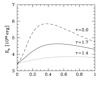
FIG. 3.: Maximum likelihood, binding energy, and $\overline{\nu}_{e}$ temperature as functions of the vacuum mixing angle. The $\overline{\nu}_{\mu}$ temperature is given by $T_{\overline{\nu}_{\mu}}=\tau\,T_{\overline{\nu}_{e}}$ with the indicated $\tau$ values.

B Vacuum Oscillations

Next, we study the case of vacuum oscillations which is relevant for small neutrino mass differences ($\Delta m^{2}\lesssim 10^{-10}\,\rm eV^{2}$). The swap probability $p$ is given by the simple formula Eq. (8) which depends only on the vacuum mixing angle so that no explicit dependence on $\Delta m^{2}$ obtains. In analogy to the $\overline{\nu}_{e}$’s we describe the time-integrated $\overline{\nu}_{\mu}$ flux by a Maxwell-Boltzmann spectrum with the same total energy, but with a higher effective temperature $T_{\overline{\nu}_{\mu}}=\tau\,T_{\overline{\nu}_{e}}$, where the factor $\tau$ is predicted to lie in the range 1.4–2.0.

We begin by performing the maximum-likelihood analysis for a fixed vacuum mixing angle and a fixed $\tau$-factor while allowing $E_{\rm b}$ and $T_{\rm\overline{\nu}_{e}}$ to float. In Fig. 3 we show as a function of $\sin^{2}2\Theta_{0}$ the maximum likelihood and the best-fit $E_{\rm b}$ and $T_{\rm\overline{\nu}_{e}}$. We show these curves for $\tau=1.4$, 1.7, and 2.0.

For $\tau=2.0$ our results agree well with those of Kernan and Krauss [14]. The maximum-likelihood curve has a maximum for $\sin^{2}2\Theta_{0}\approx 0.5$ so that a relatively large mixing angle appears to be favored by the data. The inferred SN parameters and expected detector signals for this case are summarized in Tab. I. In Fig. 3 the inferred best-fit binding energy is greater for large mixing angles compared to the no-mixing case, while the best-fit spectral temperature is a monotonically decreasing function of $\sin^{2}2\Theta_{0}$. For $\sin^{2}2\Theta_{0}\gtrsim 0.5$ and $\tau=2.0$ the best-fit $\langle E_{\overline{\nu}_{e}}\rangle$ is below $6\,{\rm MeV}$. Such a value is far below what is predicted theoretically so that it looks like large mixing angles are difficult to reconcile with the SN 1987A data.

We can also fix the binding energy and neutrino temperature according to theoretical predictions. Figure 4 shows $\ln({\cal L})$ for $E_{\rm b}=3\times 10^{53}\,{\rm erg}$ and $\langle E_{\overline{\nu}_{e}}\rangle=14\,{\rm MeV}$ as a function of the mixing angle for several values of the relative $\overline{\nu}_{\mu}$ temperature. The likelihood is a monotonically decreasing function of $\sin^{2}2\Theta_{0}$ so that, taking the predicted SN parameters seriously, the best-fit mixing angle is zero, and large mixing angles are disfavored. For $\tau=1.4$ the 95.4% confidence interval is $0\leq\sin^{2}2\Theta_{0}\leq 0.17$.

FIG. 4.: Likelihood for a fixed $E_{\rm b}=3\times 10^{53}\,{\rm erg}$ and $\langle E_{\overline{\nu}_{e}}\rangle=14\,{\rm MeV}$ as a function of the vacuum mixing angle. The $\overline{\nu}_{\mu}$ temperature is given by $T_{\overline{\nu}_{\mu}}=\tau\,T_{\overline{\nu}_{e}}$ with the indicated $\tau$ values.

Suppose that future experiments will establish vacuum oscillations as a solution of the solar neutrino problem. What would this imply for the SN 1987A parameters? To study this question we show in Fig. 5 the 95.4% confidence contours in the $T_{\rm\overline{\nu}_{e}}$-$E_{\rm b}$-plane for a joint analysis between the detectors with $\sin^{2}2\Theta_{0}=1$ and with $\tau=1.0$, $1.4$, $1.7$, and $2.0$.

FIG. 5.: Best-fit values for $T_{\overline{\nu}_{e}}$ and $E_{\rm b}$, and contours of constant likelihood which correspond to 95.4% confidence regions. In each case a joint analysis between both detectors was performed with $\sin^{2}2\Theta_{0}=1$ and the indicated relative $\overline{\nu}_{\mu}$ temperature $\tau$. The hatched region corresponds to the theoretical predictions of Eqs. (1) and (2).

The 1.0 case corresponds to no mixing; the contour is identical with that of the lower panel of Fig. 2. The maximum $\overline{\nu}_{e}$ temperature within the 95.4% confidence region is about $4.6\,{\rm MeV}$, corresponding roughly to the lower limit for the range of predicted $\langle E_{\overline{\nu}_{e}}\rangle$ values as given in Eq. (1).

For $\tau=1.4$ the 95.4% CL region for the $\overline{\nu}_{e}$ energies does not overlap with theoretical predictions. Therefore, if the vacuum solution would be borne out by future solar neutrino experiments, one would be forced to conclude that there is a significant problem with the predicted SN neutrino spectra and energies.

C Adiabatic Oscillations and Earth Effect

The most complicated case obtains if the solar neutrino problem is solved by large-angle MSW oscillations where $\Delta m^{2}\approx 10^{-5}\,\rm eV^{2}$. The propagation out of the SN is adiabatic so that no oscillations occur between there and the Earth, but we need to include regeneration effects caused by the matter-induced oscillations in the Earth. The permutation factor Eq. (9) is different for the two detectors; it is a function of the mass difference, the vacuum mixing angle and the neutrino energy.

FIG. 6.: Contours of $\Delta\ln({\cal L}_{\rm max})$, which is the maximum likelihood relative to the no-mixing value $\ln({\cal L}_{\rm max})=-41.0$. The contour lines are in steps of 1. Shaded areas correspond to $\Delta\ln({\cal L}_{\rm max})<0$, i.e. regions which are disfavored relative to the no-mixing case. The relative $\overline{\nu}_{\mu}$ temperature $\tau$ was 2.0 (upper panel) and 1.4 (lower panel).

As in Sect. IV.B we begin by performing the maximum-likelihood analysis for a fixed $\Delta m^{2}$ and $\sin^{2}2\Theta_{0}$ while allowing $E_{\rm b}$ and $T_{\overline{\nu}_{e}}$ to float. In Fig. 6 we show contours of $\ln({\cal L}_{\rm max})$ relative to the no-mixing value $\ln({\cal L}_{\rm max})=-41.0$ in steps of 1. We have used $\overline{\nu}_{\mu}$ fluences with the same total energy as for $\overline{\nu}_{e}$ and a relative temperature $\tau=2.0$ (upper panel) and $\tau=1.4$ (lower panel). The shaded areas correspond to a negative $\Delta\ln({\cal L}_{\rm max})$ and thus to a reduced likelihood relative to the no-mixing case. We emphasize that these areas cannot be interpreted as being excluded even though they are disfavored.

FIG. 7.: Contours of $\Delta\ln({\cal L}_{\rm max})$ relative to the no-mixing case for a fixed SN binding energy $E_{\rm b}=3\times 10^{53}\,\rm erg$. The contour lines are in steps of 1. Shaded areas correspond to $\Delta\ln({\cal L}_{\rm max})<0$, i.e. regions which are disfavored relative to the no-mixing case. The relative $\overline{\nu}_{\mu}$ temperature $\tau$ was 2.0 (upper panel) and 1.4 (lower panel).

For both $\tau=2.0$ and $1.4$ we find best-fit mixing parameters $\sin^{2}2\Theta_{0}=1$ and $\log(\Delta m^{2}/{\rm eV^{2}})\approx-5.5$. The absolute maximum of the likelihood is $\Delta\ln({\cal L}_{\rm max})\approx 3.7$ and $1.6$, respectively, relative to the no-mixing case. A local maximum with $\Delta\ln({\cal L}_{\rm max})\approx 1.4$ (0.4) is found for $\sin^{2}2\Theta_{0}\approx 0.8$ and $\log(\Delta m^{2}/{\rm eV^{2}})\approx-5$. The largest increase of the maximum likelihood occurs for the largest relative $\overline{\nu}_{\mu}$ temperature $\tau=2.0$. The corresponding best-fit SN parameters and expected signal characteristics are listed in Tab. I. They are far away from theoretical predictions so that the apparent improvement of the likelihood is obtained at the price of a conflict with SN theory.

FIG. 8.: Contours of $\ln({\cal L})$ in steps of 1 relative to the no-mixing case. All values are negative, i.e. the maximum is on the line $\sin^{2}2\Theta_{0}=0$. The spectral parameters were held fixed at $E_{\rm b}=3\times 10^{53}\,{\rm erg}$ and $\langle E_{\overline{\nu}_{e}}\rangle=14\,{\rm MeV}$. The relative $\overline{\nu}_{\mu}$ temperature $\tau$ was 2.0 (upper panel) and 1.4 (lower panel).

Therefore, as in Sect. IV.B we next take the opposite point of view and assume that SN theory is roughly correct so that we should keep $E_{\rm b}$ fixed at $3\times 10^{53}\,\rm erg$. In the first analysis we allow $T_{\overline{\nu}_{e}}$ to float for a fixed $\Delta m^{2}$ and $\sin^{2}2\Theta_{0}$. In Fig. 7 we show the relevant contours of the maximum likelihood relative to the no-mixing case. Again, shaded areas correspond to a diminished maximum likelihood. As in Fig. 6 the maximum likelihood has an absolute maximum for $\tau=2.0(1.4)$, $\sin^{2}2\Theta_{0}=1$ and $\log(\Delta m^{2}/{\rm eV^{2}})\approx-5.7(5.6)$ with $\Delta\ln({\cal L}_{\rm max})\approx 1.4(1.1)$. A local maximum with $\Delta\ln({\cal L}_{\rm max})\approx 0.8(0.3)$ is found for $\sin^{2}2\Theta_{0}\approx 0.8$ and $\log(\Delta m^{2}/{\rm eV^{2}})\approx-5$. A similar effect occurred in Fig. 6 where the SN binding energy was also allowed to float.

Next, we hold both spectral characteristics fixed, to wit $E_{\rm b}=3\times 10^{53}\,\rm erg$ and $T_{\overline{\nu}_{e}}=4.7\,\rm MeV$ which corresponds to the low end of the range of predicted $\langle E_{\overline{\nu}_{e}}\rangle$ values given in Eq. (1). The contours of $\ln({\cal L})$ relative to the no-mixing case are shown in Fig. 8 in steps of 1, again with $\tau=2.0$ (upper panel) and $\tau=1.4$ (lower panel). Note that all contours now represent negative $\Delta\ln({\cal L})$, i.e. diminished likelihood values. If we take the predicted SN parameters seriously we arrive at the same conclusion as in Sect. IV.B, namely that the no-mixing case is favored.

FIG. 9.: Mixing parameters favored by the MSW solutions of the solar neutrino problem and those excluded by the absence of an observed day-night effect at Kamiokande. (Contours according to Hata and Haxton [5].)

Finally, we may suppose that future experiments will establish the large-angle MSW solution of the solar neutrino problem, i.e. that the mixing parameters lie within the indicated contour of Fig. 9. Specifically, we choose the parameters $\sin^{2}2\Theta_{0}=0.8$ and $\Delta m^{2}=10^{-5}\,{\rm eV}^{2}$ with $\tau=1.0$, $1.4$, $1.7$, and $2.0$ where $\tau=1.0$ corresponds to no mixing. As in Sect. IV.B we find that the 95.4% confidence regions barely touch the lowest predicted $\overline{\nu}_{e}$ energies only in the no-mixing case. However, because of the Earth effect the other cases yield a serious conflict only when the relative $\overline{\nu}_{\mu}$ temperature is assumed to be large.

FIG. 10.: Best-fit values for $T_{\overline{\nu}_{e}}$ and $E_{\rm b}$ and contours of constant likelihood which correspond to 95.4% confidence regions. In each case a joint analysis between both detectors was performed with $\sin^{2}2\Theta_{0}=0.8$ and $\Delta m^{2}=10^{-5}\,{\rm eV}^{2}$. The curves are marked with the relative $\overline{\nu}_{\mu}$ temperature $\tau$. The hatched region corresponds to the theoretical predictions of Eqs. (1) and (2).

V Discussion and Summary

We have studied the impact of neutrino mixing on the interpretation of the SN 1987A neutrino signal, focussing on those parameter regions which are favored by the oscillation interpretation of the solar neutrino problem. For these purposes the small-angle MSW solution is equivalent to no mixing at all because only large vacuum mixing angles lead to significant modifications of the antineutrino signal from a SN. In agreement with previous authors we find that in the no-mixing case the inferred neutron-star binding energy $E_{\rm b}$ and spectral $\overline{\nu}_{e}$ temperature are consistent with theoretical predictions, but only marginally so with regard to $T_{\overline{\nu}_{e}}$; the 95.4% confidence contour in the $E_{\rm b}$-$T_{\overline{\nu}_{e}}$ plane just barely touches the predicted range of average $\overline{\nu}_{e}$ energies given in Eq. (1).

Neutrino oscillation effects lead to a partial swap of the $\overline{\nu}_{e}$ with the stiffer $\overline{\nu}_{\mu}$ spectrum. The data already point to lowish neutrino energies, especially at the Kamiokande detector, so that even a partial spectral swap aggravates the disagreement between the predicted and experimentally inferred neutrino energies.

For the large-angle MSW solution the regeneration effect in the Earth always goes in the direction of partly undoing the swap caused by the adiabatic oscillation in the SN envelope. Therefore, the 95.4% confidence contour in the $E_{\rm b}$-$T_{\overline{\nu}_{e}}$ plane may be shifted only by a small amount, depending on the exact mixing parameters, and depending on the relative $\overline{\nu}_{\mu}$ temperature (Fig. 10). Even for $\tau=T_{\overline{\nu}_{\mu}}/T_{\overline{\nu}_{e}}=2.0$ it would be difficult to claim a truly convincing conflict between observations and SN theory. Of course, the true value of $\tau$ is not known. Put another way, if the large-angle MSW solution would be borne out by future solar neutrino experiments, the observed SN 1987A signal would have to be taken as evidence for a soft $\overline{\nu}_{\mu}$ spectrum relative to the $\overline{\nu}_{e}$ one.

The solar “vacuum solution” corresponds to a very small $\Delta m^{2}$ for which the SN oscillations are not adiabatic, i.e. we have vacuum oscillations between the SN and here, and no regeneration effect in the Earth. In this case the tension between the predicted and observationally inferred SN neutrino spectra would be too significant to ignore, i.e. one would be forced to take the possibility seriously that the $\overline{\nu}_{\mu}$ spectra and/or $\overline{\nu}_{e}$ spectra are softer than had been thought previously. Conversely, if one could show that theoretical spectral predictions were accurate within the claimed range of possibilities, then one would have to agree with the findings of Smirnov, Spergel, and Bahcall [9] that the solar vacuum solution is incompatible with SN 1987A data. The conclusion of Kernan and Krauss [14] that large mixing angles were actually favored by the data can be upheld only if one ignores current theoretical predictions of the SN spectra. In this case, indeed, the likelihood function has a maximum for large mixing angles.

At the present time we would argue that the theoretical predictions of SN neutrino spectra is not well enough established to achieve a convincing selection between one of the three solutions of the solar neutrino problem. We note, for example, that current numerical calculations of the nonelectron-flavored neutrino spectra are based on energy-conserving neutrino-nucleon scatterings between their energy sphere and transport sphere in a SN core. However, nuclear recoils as well as inelastic modes of energy transfer may soften these spectra in a nonneglibile fashion [22]. There may be other novel effects which modify these spectra.

Therefore, we believe that one should view the solar neutrino experiments as one method for shedding new light on SN neutrino spectra. Of course, the most interesting case would be if one of the large-angle solutions would obtain as they would provide nontrivial new information on the spectral characteristics of the SN 1987A neutrinos.

Note Added

After this paper had been submitted for publication, a new study has appeared where the impact of gravitational fields on the phase evolution of oscillating neutrinos is investigated [23]. We believe that for the range of mixing parameters and oscillation paths considered in our paper the gravitationally induced phases do not cause an observable effect.

REFERENCES

- [1] S. P. Mikheev and A. Yu. Smirnov, Zh. Eksp. Teor. Fiz. 91, 7 (1986) [Sov. Phys. JETP 64, 4 (1986)].
- [2] K. S. Hirata, et al., Phys. Rev. Lett. 58, 1490 (1987) and Phys. Rev. D 38, 448 (1988).
- [3] R. M. Bionta et al., Phys. Rev. Lett. 58, 1494 (1987). C. B. Bratton et al., Phys. Rev. D 37, 3361 (1988).
- [4] D. Nötzold, Phys. Lett. B 196, 315 (1987). J. Arafune, M. Fukugita, T. Yanagida, and M. Yoshimura, Phys. Lett. B 194, 477 (1987) and Phys. Rev. Lett. 59, 1864 (1987). T. P. Walker and D. N. Schramm, Phys. Lett. B 195, 331 (1987). H. Minakata, H. Nunokawa, K. Shiraishi, and H. Suzuki, Mod. Phys. Lett. A 2, 827 (1987). H. Minakata and H. Nunokawa, Phys. Rev. D 38, 3605 (1988). S. P. Rosen, Phys. Rev. D 37, 1682 (1988). T. K. Kuo and J. Pantaleone, Phys. Rev. D 37, 298 (1988).
- [5] N. Hata and W. Haxton, Phys. Lett. B 353, 422 (1995).
- [6] H.-T. Janka, in: Proceedings Vulcano Workshop 1992, Frontier Objects in Astrophysics and Particle Physics, Conf. Proc. Vol. 40 (Soc. Ital. Fis.).
- [7] H.-T. Janka, in: Proceedings of the 5th Ringberg Workshop 1989 on Nuclear Astrophysics. K. Sato and H. Suzuki, Phys. Lett. B 196, 267 (1987).
- [8] L. Wolfenstein, Phys. Lett. B 194, 197 (1987). P. O. Lagage, M. Cribier, J. Rich and D. Vignaud, Phys. Lett. B 193, 127 (1987).
- [9] A. Yu. Smirnov, D. N. Spergel and J. N. Bahcall, Phys. Rev. D 49, 1389 (1994).
- [10] T. J. Loredo, D. Q. Lamb, Ann. N. Y. Acad. Sci. 571, 601 (1989).
- [11] T. J. Loredo and D. Q. Lamb, Preprint, submitted to Physical Review D, 1995.
- [12] G. Raffelt and J. Silk, Phys. Lett. B 366, 429 (1996).
- [13] V. Barger, R. J. N. Phillips, and K. Whisnant, Phys. Rev. Lett. 69, 3135 (1992). P. I. Krastev and S. T. Petcov, Phys. Rev. Lett. 72, 1960 (1994).
- [14] P. J. Kernan and L. M. Krauss, Nucl. Phys. B 437, 243 (1995).
- [15] A. Yu. Smirnov, in: V. A. Kozyarivsky (ed.), Proceedings of the Twentieth International Cosmic Ray Conference, Moscow, 1987 (Nauka, Moscow, 1987).
- [16] H.-T. Janka and W. Hillebrandt, Astron. Astrophys. 224, 49 (1989) and Astron. Astrophys. Suppl. 78, 375 (1989). P. M. Giovanoni, P. C. Ellison, and S. W. Bruenn, Astrophys. J. 342, 416 (1989). H.-T. Janka, Neutrino Transport in Type II Supernovae and Protoneutron Stars by Monte Carlo Methods, Ph. D. Thesis, Technische Universität München, MPA-Report No. 587 (1991).
- [17] S. W. Bruenn, Phys. Rev. Lett. 59, 938 (1987). R. Mayle, J. R. Wilson, and D. N. Schramm, Astrophys. J. 318, 288 (1987). A. Burrows, Astrophys. J. 334, 891 (1988). E. S. Myra and A. Burrows, Astrophys. J. 364, 222 (1990).
- [18] A. Burrows, Astrophys. J. 334, 891 (1988).
- [19] H.-T. Janka, Astropart. Phys. 3, 377 (1995).
- [20] W. T. Eadie, D. Drijard, F. E. James, M. Roos, and B. Sadoulet, Statistical Methods in Experimental Physics (North-Holland, Amsterdam, 1971).
- [21] M. G. Kendall, A. Stuart, The Advanced Theory of Statistics, Vol. 2, 4th ed. (Griffin, London 1979).
- [22] H.-T. Janka, W. Keil, G. Raffelt, and D. Seckel, Report ASTRO-PH/9507013, to be published in Physical Review Letters.
- [23] D. V. Ahluwalia and C. Burgard, E-print gr-qc/9603008 (1996), submitted to Physical Review Letters.