Constraining $\Omega_{0}$ using weak gravitational lensing by clusters

Abstract

The morphology of galaxy clusters reflects the epoch at which they formed and hence depends on the value of the mean cosmological density, $\Omega_{0}$. Recent studies have shown that the distribution of dark matter in clusters can be mapped from analysis of the small distortions in the shapes of background galaxies induced by weak gravitational lensing in the cluster potential. We construct new statistics to quantify the morphology of clusters which are insensitive to limitations in the mass reconstruction procedure. By simulating weak gravitational lensing in artificial clusters grown in numerical simulations of the formation of clusters in three different cosmologies, we obtain distributions of a quadrupole statistic which measures global deviations from spherical symmetry in a cluster. These distributions are very sensitive to the value of $\Omega_{0}$ and, as a result, lensing observations of a small number of clusters should be sufficient to place broad constraints on $\Omega_{0}$ and certainly to distinguish between the extreme values of 0.2 and 1.

1 Introduction

In a low density universe, density fluctuations cease to grow after a redshift $z\sim\frac{1}{\Omega_{0}}-1$, where $\Omega_{0}$ is the present value of the cosmological density parameter (see e.g. [Peebles (1980), §11 & §13]). Introducing a cosmological constant, $\lambda_{0}$ (which we shall express in units of $3H_{0}^{2}$, where $H_{0}$ is the present value of the Hubble constant) makes this cessation more abrupt. Hence, in low $\Omega_{0}$ models, both with and without a cosmological constant, clusters form at moderate redshift ($z$ = 1–4), and subsequently accrete very little material. In this period, which can span many dynamical times, the internal structure of the clusters relaxes to produce smooth, nearly spherical configurations. In contrast, in $\Omega_{0}=1$ models structure formation occurs continuously, rich galaxy clusters form in abundance only at very low redshift ($z$ = 0.2–0.3), and continue to accrete material even at the present epoch. Hence, if $\Omega_{0}=1$, many clusters are expected to show evidence of recent merger events and to have irregular morphologies.

Over the past few years a number of optical and X-ray studies have suggested that a significant proportion of clusters, perhaps $\sim 40\%$, show evidence of substructure (e.g. [Geller & Beers (1982), Dressler & Schectman (1988), West & Bothun (1990), Forman & Jones (1990), Bird (1994), West et al. (1995)]. Motivated by these interesting but controversial observations suggesting recent cluster growth, ?) and ?) demonstrated that, in agreement with analytic predictions [Richstone et al. (1992), Lacey & Cole (1993)], the internal structure of clusters is sensitive to the cosmological model. ?) constructed X-ray surface brightness maps from their hydrodynamic N-body simulations of cluster formation and compared these to X-ray maps of 65 clusters observed with the Einstein Imaging Proportional Counter. They concluded that galaxy clusters with the observed range of X-ray morphologies were more likely to have arisen in a high $\Omega_{0}$ cosmology.

In parallel with these developments, it has become clear that the structure of the dynamically dominant dark matter in clusters can be reliably mapped by analysing the distortions in the images of background galaxies induced by weak gravitational lensing in the cluster potential. Our aim in this paper is to assess whether the surface overdensity maps revealed by such analyses may be used to quantify cluster morphology and hence to constrain $\Omega_{0}$. To this end we simulate the lensing of background galaxies by clusters drawn from three different cosmological models. These are the same clusters studied by ?). For each cluster we create a mock CCD frame as described in ?) (hereafter WCF) and then use the inversion technique of ?) to reconstruct a map of the projected cluster overdensity.

The remainder of this paper is organised as follows. The main features of the Kaiser & Squires reconstruction method are summarized in Section 2.1. Section 2.2 introduces new statistics for measuring cluster shapes, specifically tailored to be insensitive to uncertainties inherent in the reconstructed surface overdensity maps. In Section 2.3 we describe the simulated galaxy clusters to be used as lenses and whose density profiles we examine. Section 2.4 reviews how we generate the background distribution of galaxies and create mock CCD frames of the lensed galaxies. Our results are presented in Section 3 where we compare the reconstructions to the original clusters and assess how the measured distribution of cluster shapes depends on the cosmological model. We conclude in Section 4 with a discussion and summary of our main results.

2 Methods

2.1 Lensing Reconstruction

The lensing reconstruction technique employed in this paper was devised by ?) (hereafter KS). It produces a map of the estimated overdensity, $\hat{\sigma}(\vec{\theta})$, where $\hat{\sigma}(\vec{\theta})$ is the deviation of the true cluster surface density, $\hat{S}$, from the mean surface density, $\bar{S}$, within the area being considered, measured in units of the critical surface density $S_{\rm crit}$:

$$\hat{\sigma}(\vec{\theta})=\frac{\hat{S}-{\bar{S}}}{S_{\rm{crit}}},$$ (2.1)

where $\vec{\theta}$ is the position vector on the plane of the lens. $S_{\rm crit}$ is defined as

$$S_{\rm{crit}}=\frac{c^{2}}{4\pi G}\frac{D_{\rm{os}}}{D_{\rm{ol}}D_{\rm{ls}}},$$ (2.2)

where $D$ denotes angular-diameter distance and the subscripts refer to the observer, lens and source galaxy. This critical surface density is the minimum required to produce multiple images of a source object.

As shown in WCF, the KS technique recovers the mass distribution in clusters extremely well when the lensing is weak i.e. when the bending angle varies slowly with position. Our CCD simulations in that paper demonstrated that observational complications such as seeing and noise act to diminish the reconstructed surface density. However, we showed that it was possible to correct fully for this diminution and proposed a method to estimate a multiplicative compensation factor, f.

2.2 Quantifying Shapes

Lensing reconstructions such as that of KS reliably return relative values of the surface overdensity, $\hat{\sigma}(\vec{\theta})$ (equation 2.1), but do not fix its absolute value. Since $S_{\rm crit}$ depends on the geometry of the lensing configuration through the angular-diameter distance relationship, the redshift distribution of source galaxies must be known before the mean value of $S_{\rm crit}$ (equation 2.10 below) and hence the absolute surface overdensity $\hat{S}-\bar{S}$ can be obtained from equation 2.1. In addition, the KS technique is only sensitive to variations in surface density from the mean. This is because a uniform slab of material across the whole lens plane does not distort the images of galaxies lying behind. Thus, the mean surface density, $\bar{S}$, is also unknown unless the region analysed is sufficiently large to encompass the whole of the lensing material so that the surface density near the edge of the region can be taken as the zero-point.

In order to minimise the effects of these uncertainties, we define dipole and quadrupole statistics which depend not on the absolute surface overdensity, but only on the values of $\hat{\sigma}(\vec{\theta})$ relative to each other. These statistics, therefore, are explicitly independent of $\bar{S}$, $S_{\rm crit}$ and any compensation factor $f$. We define the dipole, $D(A)$, by

$$D(A)=\frac{[d_{1}^{2}+d_{2}^{2}]^{\frac{1}{2}}}{A^{\frac{3}{2}}}=\frac{\left|d\right|}{A^{\frac{3}{2}}}$$ (2.3)

where

$$d_{1}=\int H(\hat{\sigma}-\sigma_{\rm con})x\,dA,$$ (2.4)

$$d_{2}=\int H(\hat{\sigma}-\sigma_{\rm con})y\,dA$$ (2.5)

and

$$A=\int H(\hat{\sigma}-\sigma_{\rm con})\,dA.$$ (2.6)

Here, $\sigma_{\rm con}$ is the surface overdensity of the contour level above which we choose to evaluate the statistic and $A$ is the area within that contour. $H$ is the Heaviside step function, $H(\hat{\sigma}-\sigma_{con})$, which is equal to 0 if $\hat{\sigma}<\sigma_{\rm con}$ and equal to 1 if $\hat{\sigma}\geq\sigma_{\rm con}$. The integrals are evaluated over the area within the contour. Similarly the quadrupole, $Q(A)$, for the same area $A$ is defined as

$$Q(A)=\frac{[q_{1}^{2}+q_{2}^{2}]^{\frac{1}{2}}}{A^{2}}=\frac{\left|q\right|}{A^{2}}$$ (2.7)

where

$$q_{1}=\int H(\hat{\sigma}-\sigma_{\rm con})(x^{2}-y^{2})\,dA$$ (2.8)

and

$$q_{2}=\int H(\hat{\sigma}-\sigma_{\rm con})2xy\,dA.$$ (2.9)

The $x$ and $y$ coordinates are measured relative to the cluster centre. (We shall discuss exactly how we define the cluster centre in Section 3.) In practice, the integrals become sums over pixels in the reconstructed maps. Note that both these statistics are dimensionless. If one pictures a reconstructed surface density map as a contour plot, then these statistics are independent of the value of $\hat{\sigma}$ labelling each contour because we select the contour by the area $A$ that it encloses rather than by its level. Thus, once a suitable area $A$ has been chosen, say 5 arcmin², the statistics are independent of :-

1. Any dilution of the lensing signal due to seeing.

2. Nonlinearity effects which may result in an underestimate of the surface overdensity in regions of high $\hat{S}$.

3. The (unknown) value of $S_{\rm crit}$.

The values of the statistics $D(A)$ and $Q(A)$ will, of course, depend on the noise level in the reconstructed surface density maps. It is this effect on these statistics that we aim to quantify with our simulations of lensing.

2.3 The Cluster Simulations

As our lenses we used a set of eight N-body gasdynamic simulations of the formation of galaxy clusters, further details of which may be found in ?). The clusters evolved from the same eight sets of initial density fields but in three different cosmologies:

1. A biased Einstein-de Sitter model [ $\Omega_{0}=1$, $\sigma_{8}=0.59$, where $\sigma_{8}$ is the rms fluctuation of mass within spheres of radius $8h^{-1}{\rm Mpc}$, and $h$ is the present value of the Hubble constant in units of $100$ kms^-1Mpc^-1].

2. An unbiased ($\sigma_{8}=1.0$) open model with $\Omega_{0}=0.2$ and $\lambda_{0}=0$.

3. An unbiased ($\sigma_{8}=1.0$) low density flat model with $\Omega_{0}=0.2$ and $\lambda_{0}=0.8$.

In each of four periodic boxes of size $L=15,20,25$ and $30$ $h^{-1}$ Mpc, [Evrard et al. (1994)] created two constrained realizations of Gaussian random density fields, with the standard cold dark matter power spectrum appropriate for $H_{0}=50$ km ${\rm s^{-1}}$ ${\rm Mpc^{-1}}$. In each case, using the technique of ?), they imposed the constraint that, when smoothed with a Gaussian of width $R_{f}=0.2L$, there be a peak at the centre of the box with height 2.5–5 times the rms density fluctuation on this scale.

Evrard’s (1988) P³M/SPH hydrodynamic N-body code was used to evolve the particle distributions to the present epoch. Two sets of $32^{3}$ particles represented the dark matter and gas respectively. A baryon content of $\Omega_{\rm b}=0.1$ was assumed for all the models. Gravity, PdV work and shock heating were incorporated for the gas but the effects of radiative cooling were ignored. The spatial resolution was approximately $0.005L$, varying from 75 to 150 $h^{-1}$ kpc depending on the box length. For our lensing simulations we chose the output epoch from each cosmology closest to redshift $z=0.18$. This value is fairly typical in observational studies [Wilson et al. (1996)] and corresponds to the value adopted in our previous simulations (WCF).

In the simulations of ?) the mass of each cluster was approximately proportional to the volume of the simulation box. Our aim here is to study the morphology of clusters detected by gravitational lensing with similar signal-to-noise ratio in each cosmology. Thus, for our purposes it is more convenient to have a set of clusters all of the same mass. To achieve this we simply rescaled the mass of each particle in the smaller clusters so that the total mass was the same as that in the largest cluster i.e. the one in the $L=30h^{-1}$ Mpc box. This required multiplying each mass by the factor $(30h^{-1}{\rm Mpc}/L)^{3}$. In order to preserve the correct density, we also multiplied the simulation length by $30h^{-1}{\rm Mpc}/L$.

The typical mass of a rich cluster is known approximately from observations. For a fair intercomparison of the models, the clusters considered should all have approximately the same mass within a fiducial radius such as the Abell radius ($1.5h^{-1}$Mpc). The simulated clusters in the open and flat $\Omega_{0}=0.2$ cosmologies were somewhat less massive and so we scaled them as in the previous paragraph to have approximately the same total mass as the average $\Omega_{0}=1$ cluster ($\sim 1.36\times 10^{15}h^{-1}{\rm M_{\odot}}$ within an Abell radius). The maximum scaling required was a factor of 2.4 in mass.

After this rescaling the initial conditions are no longer appropriate for a standard CDM model but instead have power spectra with slopes which differ slightly from the correct ones. However, analytic arguments show that moderate changes in the slope of the power spectrum are far less important in determining the formation history of a cluster than the actual value of $\Omega_{0}$ (Lacey & Cole 1993). Furthermore, recent high-resolution simulations of the formation of dark matter halos in an $\Omega_{0}=1$ universe by Cole & Lacey (1995) demonstrate that a statistic similar to the one we use below to characterize cluster shapes is insensitive to spectral index and halo mass (cf their Figure 17). Thus, our rescaling should have a negligible effect on our results.

We tripled the size of our cluster sample by choosing three perpendicular axes through the centre of each cluster and treating the projection along each axis as a different cluster. This resulted in 72 clusters, 24 from each of the three cosmologies.

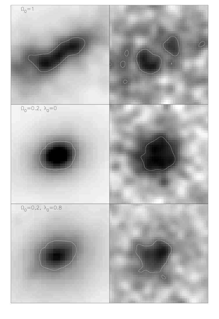
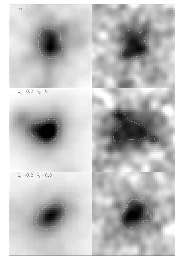
a)                                                                          b)

Figure 2: Examples of surface overdensity maps for four clusters from each of the three cosmologies. In each group the left-hand column shows the original surface density maps and the right-hand column the corresponding reconstruction. The greyscales have been adjusted according to the central surface overdensity in each case. From top to bottom the clusters are from the $\Omega_{0}=1$, open $\Omega_{0}=0.2$ and flat $\Omega_{0}=0.2$ models with the same initial fluctuation spectrum. The original CCD frame from which the reconstruction was made subtended an angle of $\sim$ 10 arcmins but these maps show only the inner 6.7 by 6.7 arcmins. At the cluster redshift, $z=0.18$, 1 arcmin is equivalent to $0.12h^{-1}$Mpc for the $\Omega_{0}=1$ cosmology. The contour plotted encloses an area of 3.8 arcmin². A Gaussian smoothing of width $\theta_{\rm sm}$ = 0.25 arcminutes has been used in the KS reconstruction procedure.

2.4 CCD images

To simulate typical observational datasets, we constructed artificial B-band CCD images of lensed field galaxies, building them up pixel by pixel, in the manner described in WCF. We employed the same distributions of galaxy ellipticity, scalelength, redshift, magnitude, noise and seeing as in that paper:

$\bullet$ Redshift and magnitude distributions

For the redshift distribution of the model galaxies, we adopted the $\rm{m_{B}}=25$ distribution predicted by the analytic model of galaxy formation of ?). Since the critical density, $S_{\rm crit}$, depends on the source redshifts through equation (2.2), we sampled this redshift distribution discretely and produced a set of source planes spanning a range of redshifts. The net effect on the reconstruction equations is that $S_{\rm crit}$ is replaced by the mean value, ${\bar{S}}_{\rm crit}$, defined by

$${\bar{S}}_{\rm crit}^{-1}=\int\frac{1}{S_{\rm crit}(z)}\,p(z)\,dz,$$ (2.10)

where $p(z)$ is the probability that a galaxy lies at redshift $z$. For our adopted redshift distribution, $\bar{S}_{\rm crit}\simeq 6\times 10^{15}h{\rm M_{\odot}/Mpc^{2}}$, with the exact value depending on the cosmology. The distribution of apparent magnitudes we generated directly from the B-band source counts of ?).

$\bullet$ Scalelength distribution

We assumed that all the background galaxies are disks with exponential profiles. The scalelength was chosen from a uniform distribution in the range 0.25 arcseconds to 0.65 arcseconds, as suggested by the observations of ?).

$\bullet$ Ellipticity distribution

Ellipticities for the background galaxies were generated by randomly sampling the empirical ellipticity distribution derived from a single frame in 0.7–0.9 arcseconds seeing by ?).

We created one CCD frame per cluster projection and then analysed it using FOCAS [Jarvis & Tyson (1981)] as described in WCF. We assumed moderately good seeing of 1 arcsecond full-width half-maximum.

3 Results

c)                                                                          d)

Figure 1. continued.

Figures 2a-d show examples of the projected mass distribution in the central regions of some of our clusters. In each group, from top to bottom, we illustrate clusters grown from identical initial conditions in the $\Omega_{0}=1$, open $\Omega_{0}=0.2$, and flat $\Omega_{0}=0.2$ cosmologies respectively. The left-hand panels give the original surface density, smoothed with a Gaussian of $\theta_{\rm sm}$ = 0.25 arcminutes, the same smoothing as we employed in the KS reconstruction. The right-hand panels show the corresponding reconstructions. The field of view in each plot is $6.7$ arcmins (equivalent to $0.8h^{-1}$ Mpc, for $\Omega_{0}=1$), and the contour on each map encloses an area of 3.8 arcmin².

The surface overdensities on the left-hand side have been normalised so that the mean value is zero over the full CCD frame, reflecting the fact that the mean value from the KS reconstruction is automatically set to zero. To enhance the substructure in the reconstructed maps, we have used different greyscales in the left- and right-hand panels. The former appear uniformly black near the centre. Limitations of scale, particularly in the open $\Omega_{0}=0.2$ case, conceal the reality that the density distribution is in fact very highly peaked. The maximum surface density can be critical or even greater. In contrast, the maximum surface overdensity in the right-hand panels is $\simeq$ 0.2 or 0.3 of critical. This diminution is partly due to observational effects such as seeing and noise, and partly due to the effects of nonlinearity - weak lensing reconstruction techniques generally underestimate $\hat{\sigma}$ in regions where the surface overdensity rises above a few tenths of critical. This failure of the method results in reconstructed profiles that saturate near the cluster centre producing a broad plateau which, in the open $\Omega_{0}=0.2$ model, extends over many hundreds of pixels with similar density values.

a)                                                                          b)

Figure 4: The quadrupole, $Q(A)$, as a function of the area over which it is calculated. Two examples are shown of clusters in each of the $\Omega_{0}=1$ (left panel) and open $\Omega_{0}=0.2$ models (right panel).

Figure 1 illustrates how clusters in the $\Omega_{0}=1$ cosmology are still forming at $z=0.18$. In most cases, large clumps are still infalling and the dominant mass condensation is usually quite elongated. By contrast, clusters in the open $\Omega_{0}=0.2$ cosmology are more centrally concentrated and closer to spherical symmetry. Clusters from the flat $\Omega_{0}=0.2$ ($\lambda_{0}=0.8$) cosmology are similar to these but they have slightly lower central overdensity and are a little more elongated. In general, the reconstructed shapes match the originals rather well. With the exception of a few noisy pixels, the essential features of the different cluster morphologies are preserved by the reconstruction.

We now use the dipole and quadrupole statistics, defined in Section 2.2, to quantify the distribution of cluster shapes in each cosmology. Initially we evaluated the statistics $D(A)$ and $Q(A)$ (equations 2.3 and 2.7) after identifying the cluster centre with the pixel of maximum surface overdensity. We found that unless the reconstructions have very high signal-to-noise, this choice of centre results in noisy estimates of $D(A)$ and to a lesser extent of $Q(A)$. For clusters with steep density profiles the reconstructed profiles have a saturated core and, as a result, the highest density peak is simply the highest noise peak anywhere in this central plateau. In light of this we tried a second choice of cluster centre which is more robust than simply selecting the densest pixel. This time we took the centre of coordinates to be the position at which $D(A)=0$ (i.e. the centroid of the area within the contour). The choice of centre now depends on the area, $A$, selected, but is much less sensitive to the presence of noise. Having chosen the centre such that $D(A)=0$ we then use only $Q(A)$ as a measure of the asymmetry of the cluster.

Figure 6: The cumulative probability distribution of the quadrupole, $Q(A)$, at a fixed area, $A$, for $A=3.8$ arcmin² (top), $6.3$ arcmin² (middle), and $12.6$ arcmin² (bottom). The cluster centre has been chosen as the point about which the dipole vanishes. The two solid lines are for the $\Omega_{0}=1$ model, the two dotted lines for the open $\Omega_{0}=0.2$ model, and the two dashed lines for the flat $\Omega_{0}=0.2$ model. In each case the curves marked by triangles correspond to the original clusters while the unmarked lines correspond to the reconstructed clusters.

Figure 4a shows $Q(A)$ as a function of area, $A$, for two clusters from the $\Omega_{0}=1$ cosmology. For $A<2$ arcmin², $Q(A)$ tends to be small because of the dominant contribution from the central relaxed core, although its value fluctuates due to noise. As larger areas (and hence smaller surface overdensities) are considered, some of the more distant infalling clumps are included and $Q(A)$ increases. $Q(A)$ then varies slowly, gradually falling as an increasing number of randomly distributed noise peaks enter into the analysis. Fig. 4b shows $Q(A)$ for two clusters from the open $\Omega_{0}=0.2$ cosmology. $Q(A)$ is fairly stable over a wide range of area, never rising above a value of $0.1$. This behaviour reflects the smooth and nearly spherical mass distribution in these clusters.

We now examine the distribution of $Q(A)$, at a fixed area $A$, for our sample of clusters in each of the 3 cosmologies. Figure 3 shows cumulative distributions of $Q(A)$ obtained from the 24 clusters in each model (see Section 2). The three panels are for $A=3.8$ arcmin², $6.3$ arcmin², and $12.6$ arcmin². The two solid lines are for $\Omega_{0}=1$, the two dotted lines for the open $\Omega_{0}=0.2$ model, and the two dashed lines for the flat $\Omega_{0}=0.2$ cosmology. For each pair, the line marked by triangles, usually with the smaller quadrupole value, corresponds to the original, smoothed clusters. The unmarked line corresponds to the reconstructed clusters. Examining the original clusters first, it is apparent that an open $\Omega_{0}=0.2$ universe forms clusters with the smallest quadrupoles, followed by the flat $\Omega_{0}=0.2$ model and finally the $\Omega_{0}=1$ case. After reconstruction, the quadrupole value tends to increase, at least for the $\Omega_{0}=1$ and the flat $\Omega_{0}=0.2$ clusters. This is primarily due to the inclusion of outlying noisy pixels in the analysis.

Figure 3 shows that even with the imperfections of the weak lensing reconstructions, there remains a strong and measurable difference in the expected distribution of cluster shapes in high and low $\Omega_{0}$ cosmologies. The dependence of these distributions on $\lambda_{0}$ is very weak and so this statistic cannot be used to constrain the cosmological constant. This does mean, however, that $\Omega_{0}$ can be constrained independently of the unknown value of $\lambda_{0}$. For example, for $A=3.8$ arcmin² we see that $75\%$ of clusters in an $\Omega_{0}=1$ universe have a $Q(A)$ value in excess of $0.1$, whereas less than $10\%$ of clusters in the two $\Omega_{0}=0.2$ universes are so aspherical. Alternatively, the median value of $Q(A)$ is approximately $0.2$ for both $A=3.8$ and $6.3$ arcmin² in the $\Omega_{0}=1$ universe, but less than $0.06$ for both the $\Omega_{0}=0.2$ universes. These large differences suggest that weak lensing observations of a small number of clusters, approximately five or so, can distinguish between these two values of $\Omega_{0}$. A larger cluster sample is required to place finer constraints on $\Omega_{0}$.

We stress that the distributions of $Q(A)$ plotted in Figure 3 are typical of those expected from KS mass reconstructions using weak lensing data obtained in realistic observing conditions. However, they are not intended to be definitive descriptions of $Q(A)$ for these cosmologies. Clearly, the exact form of the distributions will depend on the observing conditions, the seeing and limiting magnitude, as well as on the redshifts of the clusters. In practice, simulations that mimic specific observational datasets will need to be performed for this test of $\Omega_{0}$ to be reliably applied.

4 Discussion and conclusions

We have shown how global properties of the dark matter distribution in clusters, as revealed by weak gravitational lensing analyses, can be used to measure the cosmological density parameter, $\Omega_{0}$. Our approach complements and extends earlier work by ?) who first applied in practice the well established correlation between the morphology of clusters and the underlying cosmology to estimate the value of $\Omega_{0}$. Their analysis exploited the fact that the distribution of hot X-ray emitting gas in clusters is expected to reflect the structure of the underlying mass distribution. By probing this distribution directly, gravitational lensing bypasses the need to assume that the morphology of the gas faithfully mimics the morphology of the cluster mass. Possible (although unlikely) non-gravitational processes that may affect this correspondence are therefore not a concern, nor is there a worry that the test may be affected by contaminating X-ray signals from, for example, AGNs. A second advantage of the lensing approach is that it allows the matter distribution to be probed at larger cluster radii than the centrally concentrated X-ray emission, that is, at radii where the distinction between different cosmological models is particularly strong.

The major disadvantage of the lensing method is its sensitivity to projection effects. The observed galaxy shear pattern is a function of the product of the projected surface density along the line-of-sight and the effective cross-section for lensing (which depends on distance through equation 2.2). Mass clumps at large distances from the cluster contribute to the lensing signal and, in principle, to the measured quadrupole. In practice, this is unlikely to be a strong effect, particularly when the analysis is restricted to relatively small areas around the cluster centre. Nevertheless the size of this contamination needs to be assessed using different simulations from those discussed here. X-ray analyses are much less sensitive to projection effects and so the two approaches are complementary and should be used in combination.

In some respects, our detailed results must be regarded as preliminary. The simulations by [Evrard et al. (1994)] which we have analyzed have a number of limitations. Firstly, the initial conditions in all the cosmological models were laid down with the power spectrum appropriate to an $\Omega_{0}=1$ CDM universe. This inconsistency between the power spectrum and the cosmology was further exacerbated in our case by the need to rescale the simulations in order to ensure a lensing signal with comparable signal-to-noise in all cosmologies. Secondly, the baryon fraction in all the simulations was fixed to be 10% of the critical density so that in the $\Omega_{0}=0.2$ models, the gas contributes half of the total gravitating mass. Finally, the clusters we have analyzed were chosen to correspond to high peaks in the density field, but they do not represent a proper statistical sample. Although we argue that all these approximations are unlikely to affect our results significantly, it is clearly desirable to repeat our analysis with purpose-built simulations.

The main result of our work is that the distribution of a low-order statistic sensitive to global deviations from spherical symmetry in the mass distribution of clusters depends strongly on $\Omega_{0}$. The distribution of this quadrupole statistic can be robustly recovered from the shear pattern of galaxies weakly lensed by the cluster gravitational potential. We have shown that under standard observing conditions, lensing data for a handful of clusters should distinguish between cosmological models with $\Omega_{0}=1$ and $\Omega_{0}=0.2$.

This paper has been produced using the Royal Astronomical Society/Blackwell Science LaTeX style file.

References

- Bertschinger (1987) Bertschinger E., 1987, Ap.J.L., 323, L103
- Bird (1994) Bird C. M., 1994, A.J., 107, 1637
- Brainerd et al. (1995) Brainerd T. G., Blandford R. D., Smail I., 1995, preprint
- Cole et al. (1994) Cole S., Aragon-Salamanca A., Frenk C. S., Navarro J. F., Zepf S. E., 1994, M.N.R.A.S., 271, 781
- Dressler & Schectman (1988) Dressler A., Schectman S., 1988, A.J., 95, 284
- Evrard et al. (1994) Evrard A. E., Mohr J. J., Fabricant D. G., Geller M. J., 1994, Ap.J.L., 419, L9
- Forman & Jones (1990) Forman W. F., Jones C. J., 1990, in Oegerle W. R., Fitchett M. J., Danly L., ed, Clusters of Galaxies. Cambridge University Press, p. 257
- Geller & Beers (1982) Geller M. J., Beers T. C., 1982, P.A.S.P., 94, 421
- Jarvis & Tyson (1981) Jarvis J. F., Tyson J. A., 1981, A.J., 86, 476
- Kaiser & Squires (1993) Kaiser N., Squires G., 1993, Ap.J., 404, 441
- Lacey & Cole (1993) Lacey C., Cole S., 1993, M.N.R.A.S., 262, 627
- Metcalfe et al. (1995) Metcalfe N., Shanks T., Fong R., Roche N., 1995, preprint
- Mohr et al. (1995) Mohr J. J., Evrard A. E., Fabricant D. G., Geller M. J., 1995, Ap.J., 447, 8
- Peebles (1980) Peebles P. J. E., 1980, The Large-Scale Structure of the Universe. Princeton University Press
- Richstone et al. (1992) Richstone D., Loeb A., Turner E. L., 1992, Ap.J., 393, 477
- Tyson (1994) Tyson J. A., 1994, in Schaeffer R., ed, Proc. Les Houches Summer School, Cosmology and Large Scale Structure. Elsevier Scientific Publishers
- West & Bothun (1990) West M. J., Bothun G. D., 1990, Ap.J., 350, 36
- West et al. (1995) West M. J., Jones C., Forman W., 1995
- Wilson et al. (1996) Wilson G., Cole S., Frenk C. S., 1996, M.N.R.A.S., in press
- Wilson et al. (1996) Wilson G., Smail I., Frenk C. S., Ellis R. S., Couch W. J., 1996, M.N.R.A.S., in preparation