Angular Power Spectrum of the Microwave Background Anisotropy seen by the
COBE Differential Microwave Radiometer

Abstract

The angular power spectrum estimator developed by Peebles (1973) and Hauser & Peebles (1973) has been modified and applied to the 4 year maps produced by the COBE DMR. The power spectrum of the observed sky has been compared to the power spectra of a large number of simulated random skies produced with noise equal to the observed noise and primordial density fluctuation power spectra of power law form, with $P(k)\propto k^{n}$. The best fitting value of the spectral index in the range of spatial scales corresponding to spherical harmonic indices $3\leq\ell\lesssim 30$ is an apparent spectral index $n_{app}={1.13^{+0.3}_{-0.4}}$ which is consistent with the Harrison-Zel’dovich primordial spectral index $n_{pri}=1$ The best fitting amplitude for $n_{app}=1$ is ${{\langle Q_{RMS}^{2}\rangle^{0.5}}}=18\;\mu$K.

1 Introduction

The spatial power spectrum of primordial density perturbations, $P(k)$ where $k$ is the spatial wavenumber, provides evidence about processes occurring very early in the history of the Universe. In the first moments after the Big Bang, the horizon scale $ct$ corresponds to a current scale that is much smaller than galaxies, so the assumption of a scale free form for $P(k)$ on large scales is natural, which implies a power law $P(k)\propto k^{n}$. The Poisson equation $\nabla^{2}\phi=4\pi G\rho$ implies that $|\phi(k)|^{2}\propto P(k)/k^{4}$, and hence that the potential fluctuations on scale $\lambda\propto 1/k$ are $\Delta\phi^{2}\propto|\phi(k)|^{2}k^{3}\propto k^{n-1}$. Harrison (1970), Zel’dovich (1972), and Peebles & Yu (1970) all pointed out that the absence of tiny black holes implies that the limit as $k\rightarrow\infty$ of $\Delta\phi$ must be small, so $n\lesssim 1$, while the large-scale homogeneity implied by the near isotropy of the Cosmic Microwave Background Radiation (CMBR) requires that the limit as $k\rightarrow 0$ of $\Delta\phi$ must be small, so $n\gtrsim 1$. Thus the prediction of a Harrison-Zel’dovich or $n=1$ form for $P(k)$ by an analysis that excludes all other possibilities is an old one. This particular scale-free power law is scale-invariant because the perturbations in the metric (or gravitational potential) are independent of the scale. The inflationary scenario (Starobinsky 1980; Guth 1981) proposes a tremendous expansion of the Universe (by a factor $\gtrsim 10^{30}$) during the inflationary epoch, which can convert quantum mechanical fluctuations on a microscopic scale during the inflationary epoch into Gpc-scale structure now. To the extent that conditions were relatively stable during the small part of the inflationary epoch which produced the Mpc to Gpc structures we now study, an almost scale-invariant spectrum is produced (Bardeen, Steinhardt & Turner 1983). Bond & Efstathiou (1987) show that the expected variance of the coefficients $a_{\ell m}$ in a spherical harmonic expansion of the CMBR temperature given a power law power spectrum $P(k)\propto k^{n}$ is $<a_{\ell m}^{2}>\;\propto\Gamma[\ell+(n-1)/2]/\Gamma[\ell+(5-n)/2]$ for $\ell<40$. Thus a study of the angular power spectrum of the CMBR can be used to place limits on the spectral index $n$ and test the inflationary prediction of a spectrum close to the Harrison-Zel’dovich spectrum with $n=1$.

The angular power spectrum contains the same information as the angular correlation function, but in a form that simplifies the visualization of fits for the spectral index $n$. Furthermore, the off-diagonal elements of the covariance matrix have a smaller effect for the power spectrum than for the correlation function. However, with partial sky coverage the multipole estimates in the power spectrum are correlated, and this covariance must be considered when analyzing either the correlation function or the power spectrum.

The power spectrum of a function mapped over the entire sphere can be derived easily from its expansion into spherical harmonics, but for a function known only over part of the sphere this procedure fails. Wright et al. (1994) have modified a power spectral estimator from Peebles (1973) and Hauser & Peebles (1973) that allows for partial coverage and applied this estimator to the DMR maps of CMBR anisotropy. We report here on the application of these statistics to the DMR maps based on all 4 years of data (Bennett et al. 1996). Monte Carlo runs have been used to calculate the mean and covariance of the power spectrum. Fits to estimate ${\langle Q_{RMS}^{2}\rangle^{0.5}}$ and $n$ by maximizing the Gaussian approximation to the likelihood of the angular power spectrum are discussed in this paper. Since we only consider power law power spectrum fits in this paper, we use $Q$ as a shorthand for ${\langle Q_{RMS}^{2}\rangle^{0.5}}$ or $Q_{rms-ps}$, which is the RMS quadrupole averaged over the whole Universe, based on a power law fit to many multipoles. ${\langle Q_{RMS}^{2}\rangle^{0.5}}$ should not be confused with the actual quadrupole of the high galactic latitude part of the sky observed from the Sun’s location within the Universe, which is the $Q_{RMS}$ discussed by Bennett et al. (1992).

2 Estimating the Angular Power Spectrum

Wright et al. (1994) have discussed the modification of the Hauser-Peebles angular power spectrum estimator for use on CMBR anisotropy maps. To allow for the cutting out of the galactic plane, new basis functions are defined using a modified inner product:

$$<fg>={{\sum_{j=1}^{N}w_{j}f_{j}g_{j}}\over{\sum_{j=1}^{N}w_{j}}}$$ (1)

where $j$ is an index over pixels, and $w_{j}$ is the weight per pixel. In the galactic plane cut, $w_{j}=0$. We have not used weights proportional to the number of observations, so $w_{j}=1$ outside of the galactic plane cut. The custom galactic cut used in this paper basically follows $\sin|b|=1/3$ with extra cut added in Sco-Oph and Orion (Banday et al. 1996). A total of 3881 pixels are used, or 63% of the sky.

The modified Hauser-Peebles method in Wright et al. (1994) used basis functions defined using

$$G_{\ell m}=F_{\ell m}-{{F_{00}<F_{00}F_{\ell m}>}\over{<F_{00}F_{00}>}}-\sum_{m^{\prime}=-1}^{1}{{F_{1m^{\prime}}<F_{1m^{\prime}}F_{\ell m}>}\over{<F_{1m^{\prime}}F_{1m^{\prime}}>}}$$ (2)

where the $F_{\ell m}$ are real spherical harmonics and the inner product $<fg>$ is defined over the cut sphere. These functions $G_{\ell m}$ are orthogonal to monopole and dipole terms on the cut sphere. Call this the MD method since the basis functions are orthogonal to the monopole and dipole. Let the MDQ method use basis functions orthogonal to the monopole, dipole and quadrupole:

$$G^{\prime}_{\ell m}=F_{\ell m}-{{F_{00}<F_{00}F_{\ell m}>}\over{<F_{00}F_{00}>}}-\sum_{m^{\prime}=-1}^{1}{{F_{1m^{\prime}}<F_{1m^{\prime}}F_{\ell m}>}\over{<F_{1m^{\prime}}F_{1m^{\prime}}>}}-\sum_{m^{\prime}=-2}^{2}{{F_{2m^{\prime}}<F_{2m^{\prime}}F_{\ell m}>}\over{<F_{2m^{\prime}}F_{2m^{\prime}}>}}.$$ (3)

In this paper we have used the MDQ method so our results for $\ell\geq 3$ are completely independent of the quadrupole in the map. We have also tabulated the power in $\ell=2$ which is computed with $G^{\prime}_{2m}$’s which are orthogonal to the monopole, dipole, and those components of the quadrupole which occur earlier in the sequence than $m$. Because the galactic cut used is not a straight $|b|$ cut, the different $F_{2m}$’s are not quite orthogonal, and the definition of $G^{\prime}_{2m}$ depends slightly on the ordering of the $F_{\ell m}$’s. We use the ordering $1,\;\cos\phi\,\;\cos 2\phi,\;\sin\phi,\;\sin 2\phi$. With these basis functions we compute the power spectrum estimators

$${{T_{\ell}^{2}}\over{2\ell+1}}={{\sum_{m=-\ell}^{\ell}<G^{\prime}_{\ell m}T>^{2}}\over{\sum_{m=-\ell}^{\ell}<G^{\prime}_{\ell m}G^{\prime}_{\ell m}>}}$$ (4)

which are quadratic functions of the maps. Note that for full sky coverage, $T_{\ell}^{2}$ is the variance of the sky in order $\ell$, but for partial sky coverage the response of $T_{\ell}^{2}$ to inputs with $\ell^{\prime}\neq\ell$ causes $T_{\ell}^{2}$ to be larger than the order $\ell$ sky variance. Table 1 of Wright et al. (1994) shows the input-output matrix for a straight $20^{\circ}$ cut, while Table 1 shows the input-output matrix for the custom galaxy cut. The jump in Figure 5 at $\ell=5$ for the mean spectrum of $Q=17\;\mu\mbox{K},\;n=1$ inputs is caused by the off-diagonal response to $\ell=3$, while the off-diagonal response of $\ell=4$ to $\ell=2$ has been zeroed by the MDQ method.

This method computes the power spectrum, a quadratic function of the map, which includes contributions from both the true sky signal and from instrument noise. We remove the contribution of the instrument noise by subtracting the power spectrum of a noise only map. This difference map can be constructed by subtracting the two maps made from the $A$ and $B$ sides of the DMR instruments: $D=(A-B)/2$. The sum map containing the real signal is $S=(A+B)/2$. When we compute the quadratic power spectrum, we use the value $S^{2}-D^{2}=A\times B$, the power spectra reported here are the cross power spectra between the $A$ and $B$ sides of the DMR instrument.

We have computed the power spectrum of the internal linear combination “free-free free” no galaxy (NG) map (Wright et al. 1994), $T_{NG}=-0.4512T_{31}+1.2737T_{53}+0.3125T_{90}$, and the close to maximum signal-to-noise ratio maps based on $0.6T_{53}/0.931+0.4T_{90}/0.815$. The denominators in the latter expression convert the Rayleigh-Jeans differential temperatures $T_{53}$ and $T_{90}$ into thermodynamic $\Delta T$’s, but this conversion is included in the coefficients for $T_{NG}$. This process can also be applied to compute the cross power spectrum of the 53 GHz and 90 GHz maps by letting $S=(53+90)$ and $D=(53-90)$, after both maps have been converted into thermodynamic brightness temperature differences. Figure 5 shows the resulting power spectra for the three map combinations.

We have binned the power spectra in quasi-logarithmic bins in $\ell$ in order to minimize the increasing noise-to-signal ratio as $\ell$ gets large. Figure 5 and Table 2 show these binned power spectral estimates.

3 Monte Carlo Simulations

In order to calibrate and test these methods for biases, it is necessary to simulate both the cosmic variance, which gives a random map with random spherical harmonic amplitudes chosen from a Gaussian distribution with a variance determined from the chosen $Q_{in}$ and $n_{in}$, and the experimental variance, which gives the 360 million noise values needed per year. While programs to simulate the DMR time-ordered data do exist, we have not worked at this level of detail. Instead, we have used simulations that start with the maps.

The effect of noise on the map production process can be simulated using

$$T_{n}=\sigma_{1}A^{-0.5}U$$ (5)

where $\sigma_{1}$ is the noise in one observation, $U$ is an uncorrelated vector of unit variance zero mean Gaussian random variables, and $A$ is the matrix with diagonal elements $A_{ii}$ equal to the number of times the $i^{th}$ pixel was observed, and off-diagonal elements $-A_{ij}$ equal to the number of times the $i^{th}$ pixel was referenced to the $j^{th}$ pixel. Even though $A$ is singular, Wright et al. (1994) give a rapidly convergent series technique for generating noise maps. Thus each noise map depends on 6144 independent Gaussian unit variance random variables and the parameter $\sigma_{1}$.

The signal map that is added to the noise maps to give the “observed” maps is generated using independent Gaussian random amplitudes with variances given by Bond & Efstathiou (1987) for $\ell<40$. The simulations done here included $\ell$’s up to 39, so the signal map depends on 1600 Gaussian independent unit variance random variables and the two parameters $Q_{in}$ and $n_{in}$.

4 Maximum Likelihood Estimation

Using the Monte Carlo’s, we find the mean power spectrum $\overline{T_{\ell}^{2}(Q_{in},n_{in})}$, and the covariance matrix $C(Q_{in},n_{in})_{\ell\ell^{\prime}}=\langle(T_{\ell}^{2}-\overline{T_{\ell}^{2}})(T_{\ell^{\prime}}^{2}-\overline{T_{\ell}^{2}})\rangle$. For the actual power spectrum $T_{\ell}^{2}$ from the real sky or a Monte Carlo simulation, define the deviation vector $e_{\ell}=T_{\ell}^{2}-\overline{T_{\ell}^{2}(Q_{in},n_{in})}$ and the $\chi^{2}$ statistic $\chi^{2}=e^{T}C^{-1}e$. All of the fits in this paper are based on the range $\ell=\ell_{min}\ldots\ell_{max}$ with $\ell_{min}=3$ and $\ell_{max}=30$. $C$ is thus a $28\times 28$ matrix. Ignoring the quadrupole is reasonable because the galactic corrections are largest for $\ell=2$, and the maximum order used is set by the DMR beam-size of 7^∘ and the increased computer time required to analyze more orders. Since the magnitude of the covariance matrix gets larger rapidly when $Q_{in}$ increases there is a bias toward large values of $Q$ when minimizing $\chi^{2}$. One can allow for this by minimizing $-2\ln(L)$ instead of $\chi^{2}$, where $L$ is the Gaussian approximation to the likelihood:

$$-2\ln(L)=\chi^{2}+\ln(\det(C))+{\rm const}.$$ (6)

For any given power spectrum, we can adjust $Q_{in}$ and $n_{in}$ until $-2\ln L$ is minimized. This gives us the maximum likelihood fit of a power law power spectrum to the given power spectrum. We have called the values of $Q$ and $n$ that maximize the likelihood for the observed power spectrum $Q_{ML}$ and $n_{ML}$ since these are maximum likelihood values. The maximum likelihood technique gives an asymptotically unbiased determination of the amplitude $Q$ and index $n$, but only as the observed solid angle goes to infinity. Since we are limited to about 8 sr of sky, asymptotically unbiased means biased in practice, both for the quadratic statistics considered here and for linear statistics used by Górski et al. (1994) and Bond (1995). Our use of a Gaussian approximation to the likelihood for our quadratic statistics can introduce additional errors. We use our Monte Carlo simulations to calibrate our statistical methods to avoid biased final answers.

Our $k^{th}$ Monte Carlo run depends on a set of random variables $\{Z_{k}\}$ (with 1600 + 12288 elements for a cross-analysis needing two noise maps) having a known distribution, and the three parameters $Q_{in}$, $n_{in}$ and $\sigma_{1}$. $\sigma_{1}$ can be determined with great precision using the time-ordered data. Hence one needs to run many Monte Carlo simulations with several different values for $Q_{in}$ and $n_{in}$ and compare the fitted values $Q_{ML,k}$ and $n_{ML,k}$ to the fitted values for the real data, $Q_{ML,obs}$ and $n_{ML,obs}$. For the $k^{th}$ realization $\{Z_{k}\}$, the fitted values $Q_{ML,k}$ and $n_{ML,k}$ are a continuous function of the input parameters $Q_{in}$ and $n_{in}$, and one can choose values $Q_{in}=Q_{match,k}$ and $n_{in}=n_{match,k}$ such that $Q_{ML,k}=Q_{ML,obs}$ and $n_{ML,k}=n_{ML,obs}$. By choosing many different realizations of $\{Z_{k}\}$, one creates many different $(Q_{match},\;n_{match})$ pairs. Figure 5 shows this cloud of points for the 2 year $53\times 90$ cross-power spectrum, along with contours of $-2\ln L$. The spectral index we give is the median of the set of $n_{match}$’s, and the 16%-tile to 84%-tile range in $n_{match}$ defines the $\pm 1\sigma$ range. The value $1.13^{+0.3}_{-0.4}$ given in the Abstract is the weighted mean of these determinations, but we have not reduced the error because the cosmic variance is common to all three maps.

The value of ${\langle Q_{RMS}^{2}\rangle^{0.5}}$ can be found by doing a one parameter maximum likelihood fit for $Q_{ML}$ with $n$ fixed at 1. After using the Monte Carlo runs to debias the maximum likelihood results, we get the values shown in Table 3. We can also find the best fit values of $Q$ for other values of $n$. The best fit $Q$ values for $n$ forced to be 1.25 are smaller than those for $n$ forced to be 1 by an amount that allows us to estimate the effective wavenumber of our amplitude determination. We find that $\ell_{eff}=7.9$ for the 53+90 $A\times B$ case and 7.3 for the $53\times 90$ case. In Figure 5 we have chosen to plot the amplitude at $\ell=7$ which is closest to the effective wavenumber in order to minimize the correlation between the amplitude and the spectral index.

5 Discussion

The angular power spectrum of the four year COBE DMR maps has been calculated, and it is very consistent with a Harrison-Zel’dovich primordial spectrum $n_{pri}=1$, especially after the small correction for the “toe” of the Doppler peak which gives an expected apparent index of $n_{app}\approx 1.1$ for $\Omega=1$ CDM models. Models with a cosmological constant ($\Lambda$CDM) predict a smaller $n_{app}\approx 0.75$ (Kofman & Starobinsky 1985) that is still consistent with the COBE DMR observations. The amplitude derived from this analysis is in between the ${{\langle Q_{RMS}^{2}\rangle^{0.5}}}=17\;\mu$K derived from the first year maps and the ${{\langle Q_{RMS}^{2}\rangle^{0.5}}}=19\;\mu$K derived from the two year maps (Wright et al. 1994). The amplitude from the no galaxy map is consistent with but now slightly higher than the amplitude derived from the 53 and 90 GHz maps, indicating that galactic contamination is not a major problem with the chosen galactic cut.

Table 1: $10^{3}\times$ the mean over $m$ of the power spectra of $F_{\ell^{\prime}m}$ for the custom galaxy cut.

$\ell^{\prime}$	2	3	4	5	6	7	8	9	10	11	12	13	14	15	16	17	18	19
0	0	0	0	0	0	0	0	0	0	0	0	0	0	0	0	0	0	0
1	0	0	0	0	0	0	0	0	0	0	0	0	0	0	0	0	0	0
2	1087	0	0	0	0	0	0	0	0	0	0	0	0	0	0	0	0	0
3	0	1016	0	275	1	84	1	21	1	15	1	16	1	12	1	7	1	5
4	150	0	930	0	295	1	81	1	20	1	17	1	17	1	12	1	7	1
5	0	197	1	1067	0	182	1	63	1	15	1	7	1	9	1	8	1	5
6	35	0	251	0	1051	1	179	1	57	1	12	1	6	1	9	1	7	1
7	0	46	1	138	0	1103	1	167	1	58	1	15	1	7	1	8	1	7
8	6	0	55	0	143	1	1100	1	166	1	57	1	14	1	7	1	8	1
9	0	9	1	38	0	132	1	1105	1	164	1	58	1	15	1	7	1	7
10	3	0	11	0	37	0	134	1	1102	1	165	1	58	1	15	1	6	1
11	0	5	1	7	0	38	0	135	1	1104	1	161	1	56	1	14	1	6
12	3	0	8	0	6	0	39	0	139	1	1100	1	162	1	55	1	14	1
13	0	5	0	3	0	8	0	41	0	138	1	1103	1	158	1	54	1	14
14	2	0	7	0	3	0	9	0	42	0	140	1	1102	1	158	1	54	1
15	0	3	0	3	0	4	0	9	0	41	0	138	1	1105	1	157	1	53
16	1	0	4	0	4	0	4	0	9	0	42	0	139	1	1104	1	156	1
17	0	2	0	3	0	4	0	4	0	9	0	42	0	139	1	1105	1	155
18	1	0	2	0	3	0	4	0	4	0	9	0	42	0	139	1	1105	1
19	0	1	0	1	0	3	0	4	0	4	0	10	0	42	0	139	1	1105

Table 2: Binned power spectra of the 4 yr DMR Maps.

$\ell$ Range	$\ell_{eff}$	NG $A\times B$	$53\times 90$	$53+90\;A\times B$
2	02.1	+$0.08\pm 0.68$	+$0.16\pm 0.65$	+$0.15\pm 0.60$
3	03.1	+$0.76\pm 0.70$	+$0.99\pm 0.59$	+$0.90\pm 0.57$
4	04.1	+$1.65\pm 0.76$	+$1.51\pm 0.57$	+$1.52\pm 0.56$
5-6	04.6	+$1.62\pm 0.51$	+$1.40\pm 0.35$	+$1.30\pm 0.34$
7-9	06.3	+$1.71\pm 0.52$	+$0.85\pm 0.29$	+$0.94\pm 0.28$
10-13	08.9	$-0.02\pm 0.79$	+$0.78\pm 0.33$	+$1.19\pm 0.30$
14-19	11.5	+$1.50\pm 1.42$	+$1.75\pm 0.46$	+$1.52\pm 0.40$
20-30	13.2	+$0.37\pm 4.81$	+$0.57\pm 1.39$	+$0.02\pm 1.08$

Note. — All values have been normalized to the mean for $Q=17\;\mu$K, $n=1$ Monte Carlo runs.

Table 3: Power Law Fits to 4 year DMR map power spectra.

Maps	$n_{app}$	${{\langle Q_{RMS}^{2}\rangle^{0.5}}}$ at $n_{app}=1$, $[\mu$K]
53+90 A$\times$B	$1.17^{+0.34}_{-0.41}$	$17.9^{+1.6}_{-1.6}$
53$\times$90	$1.02^{+0.44}_{-0.47}$	$17.3^{+1.6}_{-2.1}$
NG A$\times$B	$1.22^{+0.60}_{-0.71}$	$19.6^{+2.9}_{-2.6}$

Cross power spectra for the 53+90 $A\times B$, $53\times 90$ and NG $A\times B$ maps. $T_{\ell}^{2}$ measures the variance of the sky due to order $\ell$ harmonics for full sky coverage, but partial sky coverage changes the expected value slightly as seen in the curves showing the average power spectrum of $Q=17\;\mu$K, $n=1$ models in the cut sky. Values are shifted upward by 400 for NG and 900 for $53\times 90$, as shown by the horizontal lines marking zero power.

Binned cross power spectra for the 53+90 $A\times B$, $53\times 90$ and NG $A\times B$ maps, normalized to the mean power spectrum of $Q=17\;\mu$K, $n=1$ simulations, plotted on a logarithmic scale. $\ell_{eff}$ is the effective wavenumber of the bin for $n=1$. The thin curves show a CDM model with $n_{pri}=0.96$ including the effect of gravitational waves derived from Crittenden et al. (1993).

Each point is an input parameter set that is consistent with the real 4 year $53\times 90$ DMR data for a given realization of the random cosmic and radiometer variance processes. The amplitude is specified using the RMS $\Delta T$ due to $\ell=7$ spherical harmonics because $\ell_{eff}$ for this fit is 7.3. The likelihood contours are at $\Delta(-2\ln L)=1$, 4 and 9.

Figure 1:  

Figure 2:  

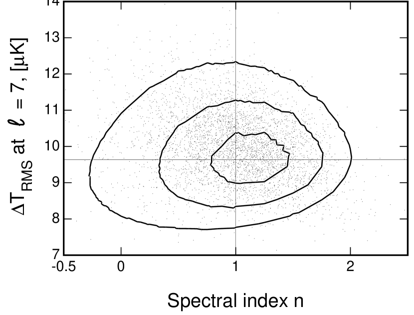
Figure 3: