Testing the LCDM model (and more) with the time evolution of the redshift

Abstract

With the many ambitious proposals afoot for new generations of very large telescopes, along with spectrographs of unprecedented resolution, there arises the real possibility that the time evolution of the cosmological redshift may, in the not too distant future, prove to be a useful tool rather than merely a theoretical curiosity. Here I contrast this approach with the standard cosmological procedure based on the luminosity (or any other well-defined) distance. I then show that such observations would not only provide a direct measure of all the associated cosmological parameters of the LCDM model, but would also provide wide-ranging internal consistency checks. Further, in a more general context, I show that without introducing further time derivatives of the redshift one could in fact map out the dark energy equation of state should the LCDM model fail. A consideration of brane-world scenarios and interacting dark energy models serves to emphasize the fact that the usefulness of such observations would not be restricted to high redshifts.

I Introduction

Differentiation of the standard cosmological redshift notation

$$1+z=\frac{a(t_{o})}{a(t_{e})}=\frac{dt_{o}}{dt_{e}}$$ (1)

gives the McVittie equation mcvittie

$$\dot{z}=H_{o}\left(1+z-\frac{H(z)}{H_{o}}\right)\equiv H_{o}Z(z),$$ (2)

where the $t$ - derivative is evaluated today. The boundary condition is $Z(0)=0$. The fact that $\dot{z}$ is very difficult to detect detect is due to the fact that $H_{o}$ is, in human terms, so very small ($\sim h\times 10^{-10}\;yr^{-1}$ with $h\equiv H_{o}/100$ and $H_{o}$ in km s^-1 Mpc^-1 where, according to all observations, $h\sim 1$). Nonetheless, almost 50 years ago Sandage sandage tried to make (2) an observational tool but concluded that this was not possible given the technology available to him. About 30 years ago Davis and May davisandmay , with appropriate caution, suggested that direct measurements of $\dot{z}$ might be feasible on timescales of decades. There have been arguments that peculiar accelerations would invalidate attempts to measure (2) phillipps countered by arguments that in a suitable sample this would not be the case lake1 . The latter argument seems to have survived and it was Loeb loeb , many years later, who pointed out that the Ly$\alpha$ absorption-line forest on the continuum flux from quasars could provide an ideal template for the observation of $\dot{z}$. Recently, Corasaniti, Huterer and Melchiorri chm have reviewed some of the many ambitious proposals afoot for new generations of very large telescopes along with spectrographs of unprecedented resolution clar . In particular, the CODEX (Cosmic Dynamics Experiment) spectrograph should be able to detect $\dot{z}$ in distant quasi-stellar objects ($z\geq 2$) over a single decade codex . It would seem that observations of $\dot{z}$ might, in the relatively short term, finally be within our grasp. However, the usefulness of such observations would, as we show here, not be restricted to high redshifts. Low redshift ($z<2$) Ly$\alpha$ systems (which requires UV space-based systems) have already produced results penton but much improvement will be needed to actually measure the low-redshift effects discussed here.

Assuming $H_{o}$ is known hubble , (2) provides cosmological information through $H(z)$. Indeed, for any background model, all properties of the model can be obtained by taking higher $t$ - derivatives of $z$ lake . However, $t$ - derivatives of order $N$ produce factors of $H_{o}^{N}$ and so this approach will remain of theoretical interest but of no practical value beyond $N=1$. Throughout the present analysis $N=1$. The approach used here is to explicitly use the redshift information contained within $Z$ itself so that no higher powers of $H_{o}$ enter. In this regard it is useful to start with a comparison of the standard approach based on luminosity (or other well-defined) cosmological distances.

II Luminosity Distances

The standard approach in cosmology is to fit measurements to a truncated Taylor series approximation to the luminosity distance which, in general, we can write as

$$d_{L}(z)=a_{o}(1+z)\mathcal{S}_{k}\left(\frac{c}{a_{o}}\int_{o}^{z}\frac{dx}{H(x)}\right)$$ (3)

where $\mathcal{S}_{k}(x)\equiv\sin(\sqrt{k}x)/\sqrt{k}$. We start with the expansion

$$H(z)=H_{o}+H^{{}^{\prime}}_{o}z+\frac{1}{2}H^{{}^{\prime\prime}}_{o}z^{2}+...$$ (4)

where ${}^{{}^{\prime}}\equiv d/dz$ (and, as usual, $H^{{}^{\prime}}_{o}$ means $dH/dz|_{z=0}$ etc.). It is customary to evaluate the coefficients in the Taylor expansion in terms of $t$ - derivatives of the scale factor evaluated at $t_{o}$. To do this consider $a_{o}$ fixed and look back along the past null cone to write the familiar relation

$$\frac{dz}{dt_{e}}=-(1+z)H(z).$$ (5)

This must not be confused with the notation used for $\dot{z}$ in (2). From (4) and (5) we obtain

$$\frac{H_{o}}{c}d_{L}(z)=\sum_{i=1}\mathcal{D}_{i}z^{i}$$ (6)

where the $\mathcal{D}_{i}$ are dimensionless constants with $\mathcal{D}_{1}=1$ but the $\mathcal{D}_{i}$ for $i>1$ contain time derivatives of the scale factor ($da/dt|_{o}$) of order up to $i$ and terms at that order of differentiation come in linearly series . Whereas the use of $d_{L}$ is standard, it is not necessarily the best distance measure to use visser . (Note, however, that the use of other distance measures merely changes the power of $(1+z)$ in (3) and this does not change the fundamentals of the procedure under discussion.) Moreover, let us note here that one need never introduce $t$ derivatives but rather one could proceed directly from (3), or any other well-defined distance. For $d_{L}$, for example, we find (6) with $\mathcal{D}_{1}=1$ but now with

$$\mathcal{D}_{2}=\frac{1}{2}(1+Z^{{}^{\prime}}_{o}),$$ (7)

and

$$\mathcal{D}_{3}=\frac{1}{6}\left(Z^{{}^{\prime\prime}}_{o}-1-Z^{{}^{\prime}}_{o}(1-2Z^{{}^{\prime}}_{o})-\frac{kc^{2}}{H_{o}^{2}a_{o}^{2}}\right)$$ (8)

and so on, where $Z$ is defined by (2) (and, as usual, $Z^{{}^{\prime}}_{o}$ means $dZ/dz|_{z=0}$ etc.). It is at this order, $\mathcal{D}_{3}$, that a degeneracy (the last term above) enters weinberg . The use of $z$ derivatives can, of course, be directly related to the more usual expansion in terms of $t$ derivatives. In particular, one easily finds

$$Z^{{}^{\prime}}_{o}=-q_{o}$$ (9)

and

$$Z^{{}^{\prime\prime}}_{o}=-j_{o}+q_{0}^{2}$$ (10)

where $q_{o}$ and $j_{o}$ are the standard deceleration and jerk parameters series . Despite what distance measure one chooses to use, the quantities $Z^{{}^{\prime}}_{o},Z^{{}^{\prime\prime}}_{o}$ and so on, enter by way of series approximation only. In the approach I discuss here, based on (2), this is not the case: encoded in $\dot{z}$, given $H_{o}$, is $Z(z)$ and therefore $Z^{{}^{\prime}}$, $Z^{{}^{\prime\prime}}$ and so on and not just their values at $z=0$. In a sense then what we consider here is a natural generalization of the cosmographic approach. The use of (2) clearly offers tremendous theoretical advantage over $d_{L}$, or other measures of distance, as (2) makes no assumptions other than the cosmological principle itself. However, we must assume a background model given, say, by way of the Friedmann function $H/H_{o}$, a standard procedure davis . In this sense the present approach differs fundamentally from the use of any distances since that approach is kinematic. In practical terms, however, it is necessary to assume that $Z(z)$, when such observations become practical, will be able to be measured with sufficient accuracy and precision in order to reliably produce derivatives. This is the central assumption made here. Whereas one should obviously never differentiate noisy data, quality data of the type needed may eventually play an important role in cosmology and the view taken here is that the associated theory is worth exploration. In what follows we consider various cosmological models and express the associated model parameters in terms of the observables, $Z$ and its $z$ derivatives. (In a very recent paper, Balbi and Quercellini bq have also explored a variety of interesting cosmological models. In terms of the present analysis, their examination is restricted to a study of $Z$ alone.) It is to be reemphasized that no series approximations are used. The resultant formulae are, albeit superficially clumsy at times, exact.

III The LCDM Model

Consider an arbitrary number of non-interacting species species so that

$$\left(\frac{H}{H_{o}}\right)^{2}=\;\sum_{i}\Omega_{io}(1+z)^{3(1+w_{i})}.$$ (11)

If we are interested in the direct measurement of cosmological parameters (say the $\Omega_{io}$ for the above model, assuming the constants $w_{i}$ are given) via $\dot{z}$ alone, then we must recognize that (2) (given (11)) provides but one equation when there are $n-1$ unknowns for $n$ species. (The boundary condition on (11) is the $z\rightarrow 0$ limit $\sum_{i}\Omega_{io}=1$.) For example, in the LCDM model (2) alone can provide unambiguous cosmological information only if the Universe is, say, assumed to be spatially flat a priori. That is, there is no test of the assumption of flatness available. The idea exploited here is to explicitly use the redshift information contained within $Z$ itself so that no higher powers of $H_{o}$ enter and to exploit this information so that we do not have to assume flatness. Specifically, in terms of the observables $Z$ and $Z^{{}^{\prime}}$ we find the following exact relations within the LCDM model:

$$\Omega_{Mo}={\frac{-2\,Z^{{}^{\prime}}z\left(2+z\right)\left(-Z+1+z\right)+2\,Z\left(z(2+z)+2-Z\left(1+z\right)\right)}{{z}^{2}\left(1+z\right)\left(3+z\right)}}$$ (12)

for the dust (including dark matter) and

$$\Omega_{\Lambda o}={\frac{-2\,Z^{{}^{\prime}}z\left(1+z\right)\left(-Z+1+z\right)+Z\left(-Z(1+3\,z)+2\,(1+z)(1+2\,z)\right)}{{z}^{2}\left(3+z\right)}}.$$ (13)

Since $\Omega_{Mo}$ and $\Omega_{\Lambda o}$ are constants, (12) and (13) provide internal consistency checks on the LCDM model as we explore $Z(z)$. Let us note that with the aide of l’Hôpital’s rule as $z\rightarrow 0$ (and note that we have to go to the second derivative), along with equations (9) and (10), we find that (12) and (13) reduce to

$$\Omega_{Mo}=\frac{2(q_{o}+j_{o})}{3}$$ (14)

and

$$\Omega_{\Lambda o}=\frac{-2q_{o}+j_{o}}{3}$$ (15)

so that $\Omega_{ko}=1-j_{o}$. Further, we have the following internal explicit test for flatness within the $\Lambda$CDM model:

$$Z^{{}^{\prime}}={\frac{Z\left(-3\,Z\left(1+z\right)^{2}+12z(1+z)+2(2z^{3}+3)\right)-{z}^{2}\left(1+z\right)\left(3+z\right)}{2\;z\left(3+z(3+z)\right)\left(-Z+1+z\right)}}.$$ (16)

Introducing the additional observable $Z^{{}^{\prime\prime}}$, we can also perform an explicit internal check on the constancy of $\Lambda$ without the assumption of flatness. In particular, it must follow from the observations that

$$Z^{{}^{\prime\prime}}={\frac{Z^{{}^{\prime}}z\left(Z^{{}^{\prime}}z\left(1+z\right)\left(3+z\right)-2\,Z\left(3+2z(3+z)\right)+2\,\left(1+z\right)\left(3+z(3+z)\right)\right)-Z\left(3\,\left(1+z\right)^{2}\left(2-Z\right)+2\,{z}^{3}\right)}{{z}^{2}\left(1+z\right)\left(3+z\right)\left(-Z+1+z\right)}}$$ (17)

or the LCDM model fails.

IV Variable Equation of State $w=w(z)$

The foregoing procedure can of course be applied to any model, not just the standard LCDM model. One popular trend today, despite the Lovelock theorem lovelock , is to generalize the LCDM model by removing the assumption that $w_{\Lambda}=-1$ and to replace it with a free (and often entirely ad hoc) constant parameter $w$. For example, under the assumption of spatial flatness we then have

$$Z=1+z-\sqrt{\left(1+z\right)^{3}\left(1-\Omega_{wo}+\Omega_{wo}(1+z)^{3\,w}\right)}\;,$$ (18)

so that

$$Z^{{}^{\prime}}(0)=-\frac{1}{2}-\frac{3}{2}\Omega_{{wo}}w$$ (19)

and

$$Z^{{}^{\prime\prime}}(0)=\frac{9}{4}\Omega_{{wo}}{w}^{2}(\Omega_{{wo}}-2)-3\Omega_{{wo}}w-\frac{3}{4}.$$ (20)

With the aide of (9) and (10) then

$$q_{0}=\frac{1}{2}+\frac{3}{2}\Omega_{{wo}}w$$ (21)

and

$$j_{0}=1+\frac{9}{2}\Omega_{{wo}}w(1+w)$$ (22)

compared with $q_{o}=1/2-3\Omega_{\Lambda o}/2$ and $j_{o}=1$ in the flat LCDM model. The situation is summarized in Figures 1 and 2. These diagrams suggest, for example, that $\Omega_{w_{o}}$ could be obtained from $Z^{{}^{\prime}}$ at high redshift and compared with $Z$ in the same redshift range. Further, $w$ might be obtained from $Z$ at high redshift and compared to $w$ obtained from $Z^{{}^{\prime}}$ and $Z^{{}^{\prime\prime}}$ at low redshift to check the assumption $w^{{}^{\prime}}=0$. Although such a comparison would require very different technologies, this comparison serves to point out that the usefulness of $\dot{z}$ observations would not be restricted to high redshifts.

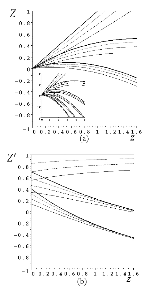
Figure 1: The functions $Z$ (part (a)) and $Z^{{}^{\prime}}$ (part (b)) under the assumption of spatial flatness and constant $w$ as follows from (18). Three values of $\Omega_{w_{o}}$ are shown; $\Omega_{w_{o}}=1,0.8,$ and $0.6$ and within each four values of $w$ are shown; $w=-1$ (wide solid), $-0.9$ (dot), $-0.8$ (dash) and $-0.7$ (thin solid). These are read top down. The insert for $Z$ also shows $\Omega_{w_{o}}=0.9,0.7,$ and $0.5$ over a wider redshift range. The case $\Omega_{w}=-w=1$ corresponds to de Sitter space. The diagrams suggest that there would be little advantage in trying to go to very high redshifts. (In any event, the Ly$\alpha$ forest disappears at $z\sim 4$).

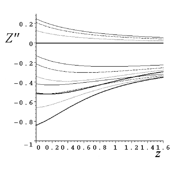
Figure 2: The function $Z^{{}^{\prime\prime}}$ under the assumption of spatial flatness and constant $w$ as follows from (18) with the same conditions as Figure 1 except that the conditions on $w$ are read bottom up.

If we assume spatial flatness and continue to use $Z,Z^{{}^{\prime}}$ and $Z^{{}^{\prime\prime}}$ as obervables then we need not assume $w$ is constant. Rather, we can actually solve for $w(z)$. In the usual way we now obtain

$$\frac{H}{H_{o}}=\sqrt{\left(1+z\right)^{3}\left(\Omega_{Mo}+\Theta(z)\Omega_{wo}\right)},$$ (23)

where

$$\Theta(z)\equiv\exp(3\int_{0}^{z}\frac{w(x)}{1+x}dx).$$ (24)

In this case writing $w=w(z)$ we find

$$\Omega_{Mo}={\frac{\left(-Z+1+z\right)\left(2\,Z^{{}^{\prime}}\left(1+z\right)-3\,Z\left(1+w\right)+\left(1+z\right)\left(3\,w+1\right)\right)}{3w\left(1+z\right)^{3}}}$$ (25)

and

$$\Omega_{wo}={\frac{-2\,Z^{{}^{\prime}}\left(1+z\right)\left(-Z+1+z\right)+Z\left(-3\,Z\left(1+w\right)+2\,\left(1+z\right)\left(3\,w+2\right)\right)+\left(1+z\right)^{2}\left(3\,zw-1\right)}{3w\left(1+z\right)^{3}}}$$ (26)

where now $w(z)$ follows from

$$w\left(z\right)=\frac{{e^{\int\!-{\frac{f\left(z\right)}{\left(1+z\right)h\left(z\right)}}{dz}}}}{\int\!3\,{e^{\int\!-{\frac{f\left(z\right)}{\left(1+z\right)h\left(z\right)}}{dz}}}\left(1+z\right)^{-1}{dz}+{\it C}}$$ (27)

where ${\it C}$ is a constant (provided by the theory that gives $w(z)$) and the observables $h(z)$ and $f(z)$ are given by

$$h(z)\equiv\left(-Z+1+z\right)\left(-3\,Z+\left(1+z\right)(1+2\,Z^{{}^{\prime}})\right)$$ (28)

and

$$f(z)\equiv-2\,Z^{{}^{\prime\prime}}\left(1+z\right)^{2}\left(-Z+1+z\right)-2\,\left(1+z\right)Z^{{}^{\prime}}\left(-(Z^{{}^{\prime}}+3)\left(1+z\right)+5\,Z\right)$$ (29)

$$+Z\left(9\,Z-8(1+z)\right)+\left(1+z\right)^{2}.$$

Note that $\Theta$ does not enter. It should be clear that the introduction of $Z^{{}^{\prime\prime\prime}}$ as an observable would allow us to map out $w(z)$ without the assumption of spatial flatness, but the associated algebra is not repeated here.

V Recovering The Flat LCDM Model

As a check of the above let us note that if we use (16) in (12) and (13), or $w(z)=-1$ and (16) in (25) and (26), we obtain the following simple forms for the flat $\Lambda$CDM model:

$$\Omega_{Mo}={\frac{\left(-Z+2+z\right)\left(-Z+z\right)}{z\left(3+z(3+z)\right)}}$$ (30)

and

$$\Omega_{\Lambda o}={\frac{Z\left(-Z+2(1+z)\right)+z\left(1+z\right)^{2}}{z\left(3+z(3+z)\right)}}$$ (31)

so that now the $z\rightarrow 0$ limit gives us the familiar relations (14) and (15) with $j_{0}=1$. Similarly, substituting from (16) into (17), or $w(z)=-1$ into the derivative of (27) and using (16), we obtain

$$Z^{{}^{\prime\prime}}={\frac{3\left(1+z\right)\left(-Z+z\right)\left(-Z+2+z\right)\left(Z\left(3(\,z-1)+{z}^{2}\left(3+z\right)\right)\left(Z-2(1+z)\right)+z\left(6+z\left(3+z\right)\right)\left(1+z\right)^{2}\right)}{4{z}^{2}\left(Z-1-z\right)^{3}\left(3(1+\,z)+{z}^{2}\right)^{2}}}$$ (32)

which, in addition to a check on the foregoing, reiterates the fact that the only observable needed in the flat LCDM case is $Z$ alone.

VI Acceleration Without $\Lambda$

The idea that the accelerated Universe could be the result of extra dimensions - for example, the so-called DGP models dgp , is widely discussed in the literature. Cosmological tests based on $d_{L}$ in these models have been studied by Deffayet, Dvali and Gabadadze deffayet and more recently by Maartens and Majerotto maartens . Here we consider the spatially flat case so that we need only consider $Z$. In this model we have

$$\frac{H}{H_{o}}=\frac{(1-\Omega_{Mo})}{2}+\sqrt{\left(\frac{(1-\Omega_{Mo})}{2}\right)^{2}+\Omega_{Mo}(1+z)^{3}}$$ (33)

so that subject to the boundary condition $Z(0)=0$ we have

$$Z=\frac{\Omega_{Mo}+1}{2}+z-\sqrt{\left(\frac{\Omega_{Mo}+1}{2}\right)^{2}+\Omega_{Mo}z\left(3+3\,z+{z}^{2}\right)}$$ (34)

so that

$$Z^{{}^{\prime}}(0)=\frac{1-2\Omega_{Mo}}{\Omega_{Mo}+1}$$ (35)

and

$$Z^{{}^{\prime\prime}}(0)=\frac{6\Omega_{Mo}(3\Omega_{Mo}-(\Omega_{Mo}+1)^{2})}{(\Omega_{Mo}+1)^{3}}.$$ (36)

Again with the aide of (9) and (10) we now have

$$q_{o}={\frac{2\,\Omega_{{Mo}}-1}{\Omega_{{Mo}}+1}}$$ (37)

and

$$j_{o}={\frac{10\,{\Omega_{{Mo}}}^{3}+3\,\Omega_{{Mo}}+1-6\,{\Omega_{{Mo}}}^{2}}{\left(\Omega_{{Mo}}+1\right)^{3}}}.$$ (38)

Relation (34) can be compared with the spatially flat LCDM model where from (30) we obtain

$$Z=z+1-\sqrt{1+\Omega_{{Mo}}z\left(3+3\,z+{z}^{2}\right)}$$ (39)

so that $q_{o}=3\Omega_{Mo}/2-1$ and of course $j_{o}=1$. A comparison is carried out in Figures 3 and 4. The most noticeable feature is perhaps the fact that for the same $\Omega_{Mo}$ the models predict rather different values for $q_{o}$ and $j_{o}$.This again serves to point out that the usefulness of $\dot{z}$ observations would not be restricted to high redshifts.

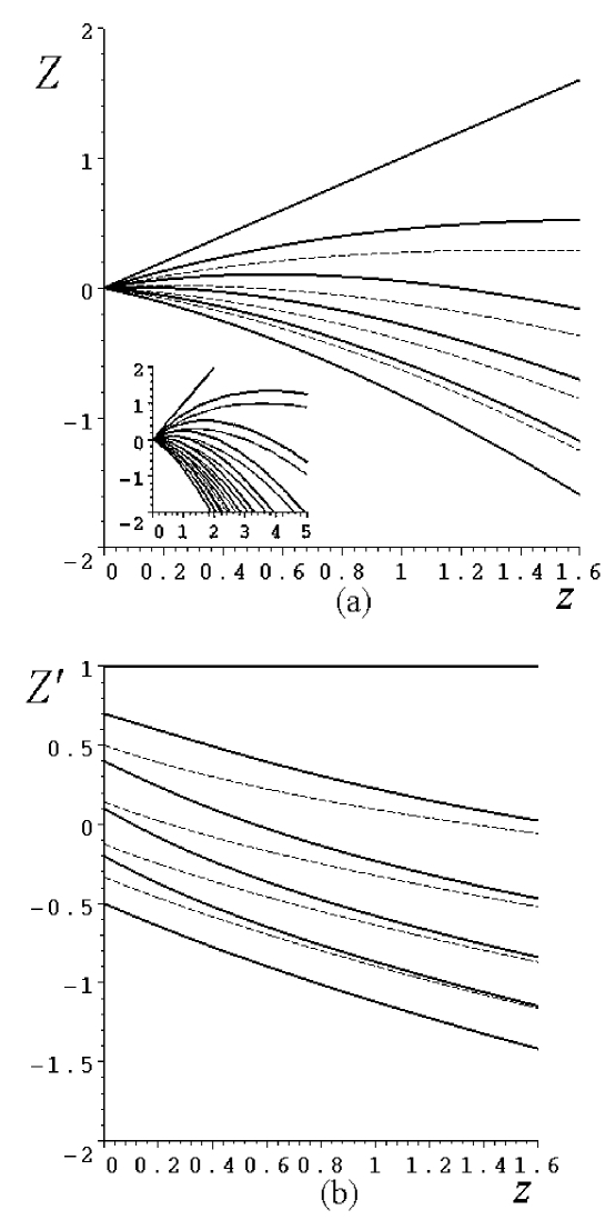
Figure 3: The functions $Z$ (part (a)) and $Z^{{}^{\prime}}$ (part (b)) as follows from (34) and (39). The LCDM model corresponds to the solid lines. In all cases $\Omega_{Mo}$ varies from $1$ (bottom coincident curve, that is the Einstein-de Sitter universe) to $0$ (top coincident curve, that is de Sitter space) in intervals of $0.2$. The insert for $Z$ also shows more values of $\Omega_{Mo}$ over a wider redshift range.

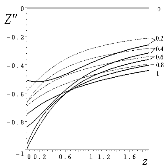
Figure 4: The function $Z^{{}^{\prime\prime}}$ from (34) and (39) with the same conditions as Figure 3. The values of $\Omega_{Mo}$ are shown on the right.

VII Interacting dark energy

It is natural to consider the coupling between dark energy and matter and there are many explicit coupling procedures considered in the literature. Here we use the parametrization of Majerotto, Sapone and Amendola majerotto to write

$$\left(\frac{H}{H_{\;o}}\right)^{2}=\Omega_{k}(1+z)^{2}+(1+z)^{3}(1-\Omega_{k})\left(1-\frac{\Omega_{de}}{1-\Omega_{k}}(1-(\frac{1}{1+z})^{\xi})\right)^{\frac{-3w}{\xi}}$$ (40)

and setting $w=-1$, $\delta=3/\xi$ and considering the spatially flat case we have

$$Z=1+z-\sqrt{(1+z)^{3}\left(\Omega_{Mo}+(1-\Omega_{Mo})\left(\frac{1}{1+z}\right)^{\frac{3}{\delta}}\right)^{\delta}}$$ (41)

so that with $\delta=1$ we recover the LCDM model and (41) reduces to (39). We now have

$$Z^{{}^{\prime}}(0)=1-\frac{3\Omega_{Mo}}{2},$$ (42)

exactly as in the LCDM model, and

$$Z^{{}^{\prime\prime}}(0)=\frac{3\Omega_{Mo}(6(\Omega_{Mo}-1)+2\delta(1-\frac{3\Omega_{Mo}}{2}))}{4\delta}.$$ (43)

Again with the aide of (9) and (10) we now have

$$q_{o}=\frac{3\Omega_{Mo}}{2}-1$$ (44)

and

$$j_{o}={\frac{9\,{\Omega_{Mo}}^{2}\left(\delta-1\right)-9\,\Omega_{Mo}\left(\delta-1\right)+2\,\delta}{2\delta}}.$$ (45)

A comparison is carried out in Figures 5 and 6.

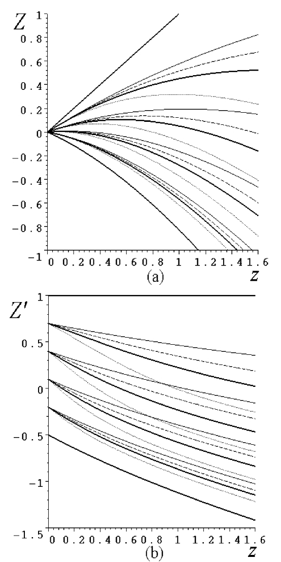
Figure 5: The functions $Z$ (part (a)) and $Z^{{}^{\prime}}$ (part (b)) as follows from (41). In all cases $\Omega_{Mo}$ varies from $1$ (bottom coincident curve, that is the Einstein-de Sitter universe) to $0$ (top coincident curve, that is de Sitter space) in intervals of $0.2$. Within each value of $\Omega_{Mo}$ four values of $\delta$ are shown; $\delta=0.75$ (dot), $1$ (thick solid = LCDM), $1.2$ (dash) and $1.5$ (thin solid).

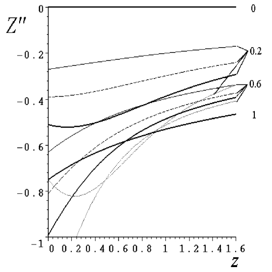
Figure 6: The function $Z^{{}^{\prime\prime}}$ from (41) with the same conditions as Figure 5. The values of $\Omega_{Mo}$ are shown on the right.

VIII Discussion

Measurements of $\dot{z}$ of sufficient quality, without the introduction of further time derivatives, would not only allow a detailed verification of the LCDM model with a minimum number of assumptions, but also a mapping of the dark energy equation of state $w(z)$ should the LCDM model fail. The procedure given here can be immediately applied to any model for which $H(z)/H_{o}$ can be written out explicitly. A consideration of brane-world scenarios and interacting dark energy models serves to emphasize the fact that the usefulness of such observations would not be restricted to high redshifts.