Strong lensing optical depths in a $\Lambda$CDM universe

Abstract

We investigate strong gravitational lensing in the concordance $\Lambda$CDM cosmology by carrying out ray-tracing along past light cones through the Millennium Simulation, the largest simulation of cosmic structure formation ever carried out. We extend previous ray-tracing methods in order to take full advantage of the large volume and the excellent spatial and mass resolution of the simulation. As a function of source redshift we evaluate the probability that an image will be highly magnified, will be highly elongated or will be one of a set of multiple images. We show that such strong lensing events can almost always be traced to a single dominant lensing object and we study the mass and redshift distribution of these primary lenses. We fit analytic models to the simulated dark halos in order to study how our optical depth measurements are affected by the limited resolution of the simulation and of the lensing planes that we construct from it. We conclude that such effects lead us to underestimate total strong-lensing cross sections by about 15%. This is smaller than the effects expected from our neglect of the baryonic components of galaxies. Finally we investigate whether strong lensing is enhanced by material in front of or behind the primary lens. Although strong lensing lines-of-sight are indeed biased towards higher than average mean densities, this additional matter typically contributes only a few percent of the total surface density.

1 Introduction

Gravitational lensing was first discovered through strong lensing effects which can produce multiple images of distant quasars (Walsh et al., 1979) and highly distorted images of distant extended objects such as galaxies (Lynds & Petrosian, 1986; Soucail et al., 1987) and radio sources (Hewitt et al., 1988). Such effects occur when the surface mass density of an individual object (the ‘lens’) is comparable to that across the Universe as a whole, and as a result they are generated only by the most massive and most concentrated structures. In contrast, weak lensing, detected through the small but coherent distortion of the images of distant galaxies in the same direction on the sky (Tyson et al., 1990), is sensitive to the abundance and structure of typical nonlinear objects, so-called dark matter halos, and is now beginning to measure the statistics of the cosmic mass distribution also in the quasilinear regime (Semboloni et al., 2006; Hoekstra et al., 2006; Hetterscheidt et al., 2007; Massey et al., 2007). Thus gravitational lensing complements microwave background, large-scale structure, and Ly$\alpha$ forest studies, which provide information primarily in the quasilinear and linear regimes (for recent reviews on strong and weak lensing, see Kochanek, 2006; Schneider, 2006b). Combining all these measures to constrain theories for the origin of structure requires a reliable model for the nonlinear phases of evolution.

The current standard model of cosmological structure formation is based on cold dark matter and a cosmological constant. This $\Lambda$CDM model has been shown to fit a wide variety of observations of galaxies and their dark halos, of galaxy clusters and galaxy clustering, of the structure of the intergalactic medium out to redshift 6, and, most notably, of the detailed pattern of temperature fluctuations in the cosmic microwave background. The parameters of the model are already highly constrained (Spergel et al., 2007). Early predictions for its lensing properties were based on analytic models for nonlinear structure (e.g. Turner et al., 1984; Subramanian et al., 1987; Narayan & White, 1988), but reliable predictions require numerical simulation (e.g. Bartelmann et al., 1998; Jain et al., 2000; Wambsganss et al., 2004). Recent gravitational lensing work has confirmed the dark halo structure predicted by these simulations for galaxies (Hoekstra et al., 2002; Seljak et al., 2005; Mandelbaum et al., 2006b; Simon et al., 2007) and clusters (Comerford et al., 2006; Mandelbaum et al., 2006a; Natarajan et al., 2007) as well as for the ensemble properties of the dark halo population (Semboloni et al., 2006; Hoekstra et al., 2006). Substantial efforts are currently underway to improve all these measurements, and these will need to be matched by a comparable improvement in the theoretical predictions.

Additional tests and constraints may be obtained from observations of gravitational lensing effects. For example, foreground matter inhomogeneities may (de-)magnify images of distant sources thus changing their apparent magnitude. Although expected to be small for current type Ia supernova samples (Wambsganss et al., 1997; Holz, 1998; Riess et al., 1998; Valageas, 2000; Amanullah et al., 2003; Knop et al., 2003; Barris et al., 2004; Riess et al., 2004), some evidence for lensing effects on the observed luminosity distribution may be present in higher-redshift samples (Wang, 2005; Jönsson et al., 2006). For future supernova surveys, one should be able to detect such effects with higher statistical significance (Metcalf, 1999; Metcalf & Silk, 1999; Minty et al., 2002; Munshi & Valageas, 2006). This will then provide a further test of the standard structure formation model.

Sufficiently massive and concentrated structures along the line-of-sight can give rise to multiple images, to strongly magnified images and to highly distorted images, so-called giant arcs. The number of such strong-lensing events depends on the abundance of massive objects and on their detailed internal structure, both of which are sensitive to the background cosmology. Currently a much-debated question is whether the observed frequency of giant arcs (Luppino et al., 1999; Zaritsky & Gonzalez, 2003; Gladders et al., 2003) is too high compared to predictions based on $\Lambda$CDM models with parameters favoured by other observations (Bartelmann et al., 1998; Meneghetti et al., 2000; Oguri et al., 2003; Dalal et al., 2004; Wambsganss et al., 2004; Li et al., 2005; Horesh et al., 2005; Li et al., 2006; Wu & Chiueh, 2006; Meneghetti et al., 2007). The problem appears particularly pressing at higher redshift, but available simulation results are not good enough to establish a clear discrepancy.

In this paper, we will study the optical depth for a variety of strong lensing effects as a function of source redshift in the standard $\Lambda$CDM cosmology. In particular, we will estimate the fraction of images that are highly magnified by gravitational lensing, that have a large length-to-width ratio, or that belong to multiply imaged sources. In addition, we compare the effect of foreground and background matter to that of the primary lens in generating these optical depths.

The results presented here were obtained by shooting random rays through a series of lens planes created from the Millennium Simulation (Springel et al., 2005). This very large $N$-body simulation of cosmic structure formation covers a volume comparable to the largest current surveys with substantially better resolution than previous simulations used for ray-tracing studies. Our set of lens planes represents the entire mass distribution between source and observer, allowing us to quantify the effects of foreground and background matter. In addition we have ensured that our ray-tracing techniques take full advantage both of the statistical power offered by the large volume of the simulation, and of its high spatial and mass resolution. This allows us to make more precise statements about model expectations than has previously been possible.

Our paper is organised as follows. In Sec. 2, we describe how we trace representative rays through the Millennium Simulation. Results for the magnification distribution as a function of source redshift are presented in Sec. 3.1. Strong-lensing optical depths are then discussed in Sec. 3.2. In Sec. 3.3, the mass and redshift distribution of the objects which cause strong lensing are examined, and we demonstrate that the errors induced by the finite volume and resolution of the simulation are relatively small. Biases induced by additional structure in front of or behind the principal lens are examined in Sec. 3.4 and are also found to be small. The paper concludes with a summary and outlook in Sec. 4.

2 Methods

2.1 The multiple-lens-plane approximation

In the multiple-lens-plane approximation (see, e.g., Blandford & Narayan, 1986; Schneider et al., 1992), a finite number of planes are introduced along the line of sight, onto which the matter inhomogeneities in the backward light cone of the observer are projected. Between these lens planes, light is assumed to travel on straight lines. Light rays are deflected only when passing through a lens plane. The deflection angles may be calculated from the gradient of a lensing potential, which is connected to the projected matter distribution on the lens planes via a Poisson equation.

A light ray reaching the observer from a given angular position $\bm{\theta}$ can then be traced back to the angular position $\bm{\beta}$ of its source at given redshift $z^{\mathrm{S}}$, thereby defining the lensing map

$$\mathrm{L}:\;\mathbb{P}^{\mathrm{I}}\to\mathbb{P}^{\mathrm{S}}:\;\bm{\theta}\mapsto\bm{\beta}$$ (1)

from the image plane $\mathbb{P}^{\mathrm{I}}$ to the source plane $\mathbb{P}^{\mathrm{S}}$. The distortion matrix $\bm{\mathsf{A}}=\frac{\partial\bm{\beta}}{\partial\bm{\theta}}$, i.e. the Jacobian of the map, quantifies the magnification and distortion of images of small sources induced by gravitational lensing. The (signed) magnification $\mu$ of an image is given by the inverse determinant of the distortion matrix:

$$\mu=\left(\det{\bm{\mathsf{A}}}\right)^{-1}.$$ (2)

The decomposition (Schneider et al., 1992)

$$\bm{\mathsf{A}}=\begin{pmatrix}\cos\varphi&\sin\varphi\\ -\sin\varphi&\cos\varphi\end{pmatrix}\begin{pmatrix}1-\kappa-\gamma_{1}&-\gamma_{2}\\ -\gamma_{2}&1-\kappa+\gamma_{1}\end{pmatrix}$$ (3)

of the distortion matrix defines the image rotation angle $\varphi$, the convergence $\kappa$, and the complex shear $\gamma=\gamma_{1}+\mathrm{i}\gamma_{2}$. The reduced shear $g=\gamma/(1-\kappa)$ determines the major-to-minor axis ratio

$$r=\left|\frac{1+|g|}{1-|g|}\right|$$ (4)

of the elliptical images of sufficiently small circular sources. The determinant and trace of the distortion matrix may be used to categorise images (Schneider et al., 1992):

• type I: $\det\bm{\mathsf{A}}>0$ and $\mathrm{tr}\,\bm{\mathsf{A}}>0$,

• type II: $\det\bm{\mathsf{A}}<0$,

• type III: $\det\bm{\mathsf{A}}>0$ and $\mathrm{tr}\,\bm{\mathsf{A}}<0$.

In all situations relevant for this work, images of type II and type III belong to sources that have multiple images. In the following, we will often consider type II and III images together as

• type $\mathrm{II}\vee\mathrm{III}$: $\det\bm{\mathsf{A}}<0$ or $\mathrm{tr}\,\bm{\mathsf{A}}<0$.

In this paper, we want to study how often one can expect to observe images with certain lensing properties, e.g. highly magnified or strongly distorted images. In order to quantify the frequency of rays with a given property $p$, we define the optical depth

$$\tau^{\mathrm{I}}_{p}=\frac{\int_{\mathbb{P}^{\mathrm{I}}}\mathrm{d}^{2}{\bm{\theta}}\,1_{p}(\bm{\theta})}{\int_{\mathbb{P}^{\mathrm{I}}}\mathrm{d}^{2}{\bm{\theta}}\,},$$ (5)

where

$$1_{p}(\bm{\theta})=\begin{cases}1&\text{if ray}(\bm{\theta})\text{ has property }p,\text{ or}\\ 0&\text{otherwise.}\end{cases}$$

For a uniform distribution of images in the image plane, $\tau^{\mathrm{I}}_{p}$ estimates the fraction of images of sufficiently small sources that have the property $p$. Furthermore, we define the optical depth

$$\tau^{\mathrm{S}}_{p}=\frac{\int_{\mathbb{P}^{\mathrm{I}}}\mathrm{d}^{2}{\bm{\theta}}\,\left|\mu(\bm{\theta})\right|^{-1}1_{p}(\bm{\theta})}{\int_{\mathbb{P}^{\mathrm{I}}}\mathrm{d}^{2}{\bm{\theta}}\,\left|\mu(\bm{\theta})\right|^{-1}}$$ (6)

to estimate the average fraction of images with properties $p$ for a uniform distribution of sources in the source plane. These optical depths (assumed to be smooth) will be used to define corresponding probability density functions (pdf) for the magnification:

$$\mathrm{pdf}^{\mathrm{I/S}}(\mu^{\prime})=\frac{\mathrm{d}}{\mathrm{d}\mu^{\prime}}\tau^{\mathrm{I/S}}_{\mu(\bm{\theta})\leq\mu^{\prime}}\;.$$ (7)

Compared to $\tau^{\mathrm{I}}_{p}$, the optical depth $\tau^{\mathrm{S}}_{p}$ takes into account that areas in the image plane with higher magnification map to smaller areas in the source plane. This aspect of magnification bias leads to a lower image density in areas of higher magnification for volume-limited surveys. In magnitude-limited surveys, however, magnification can push images that would otherwise be too faint to be observed above the detection threshold. This aspect of magnification bias counteracts the previous one, but will not be discussed in this paper since it depends sensitively on the luminosity distribution of the source population.

Note that $\tau^{\mathrm{I}}_{p}$ and $\tau^{\mathrm{S}}_{p}$ differ from the optical depths

$$\tilde{\tau}^{\mathrm{S}}_{p}=\frac{\int_{\mathbb{P}^{\mathrm{S}}}\mathrm{d}^{2}{\bm{\beta}}\,1_{p}(\bm{\beta})}{\int_{\mathbb{P}^{\mathrm{S}}}\mathrm{d}^{2}{\bm{\beta}}\,}.$$ (8)

discussed, e.g., by Schneider et al. (1992), which quantify the fraction of sources whose images have certain properties. The methods used in this paper do not yield enough information to deduce $\tilde{\tau}^{\mathrm{S}}_{p}$ in general. We will therefore restrict our discussion to $\tau^{\mathrm{I}}_{p}$ and $\tau^{\mathrm{S}}_{p}$.

Roughly speaking, $\tau^{\mathrm{I}}_{p}$ weights lensing events by their area on the sky, $\tau^{\mathrm{S}}_{p}$ weights by the number of images, and $\tilde{\tau}^{\mathrm{S}}_{p}$ weights by the number of sources. In the absence of multiple images, $\tau^{\mathrm{S}}_{p}$ and $\tilde{\tau}^{\mathrm{S}}_{p}$ would be identical. For strongly lensed properties such as considered in this paper, they can be significantly different: For $\tau^{\mathrm{S}}_{p}$, each of the multiple images of a source contributes individually, whereas all images of the same source contribute a single event event to $\tilde{\tau}^{\mathrm{S}}_{p}$. Consequently, for a given number $N^{S}$ of uniformly distributed sources in the source plane, $N^{S}\tau^{\mathrm{S}}_{p}$ is the expected number of images with property $p$, whereas $N^{S}\tilde{\tau}^{\mathrm{S}}_{p}$ gives the expected number of sources. Obviously, the number of images is easier to count in observations than the number of sources.

2.2 The lens planes

Our methods for reconstructing the observer’s backward light cone, for splitting it into a series of lens planes, and for calculating the matter distribution and deflection angles on these planes are generally similar to those used by Jain et al. (2000). They differ, however, in a number of important details which reflect our wish to take full advantage of the unprecedented statistical power offered by the large volume and high spatial and mass resolution of the Millennium Simulation. Here, we give a brief outline of our algorithms, reserving a detailed description for Hilbert et al. (2007).

The Millennium Simulation (Springel et al., 2005) is an $N$-body simulation of cosmological structure formation in a flat $\Lambda$CDM universe with a matter density of $\Omega_{\mathrm{M}}=0.25$ (in terms of the critical density), a cosmological constant with $\Omega_{\Lambda}=0.75$, a Hubble constant $h=0.73$ in units of $100\,\mathrm{km}\mathrm{s}^{-1}\mathrm{Mpc}^{-1}$, a primordial spectral index $n=1$ and a normalisation parameter $\sigma_{8}=0.9$ for the linear density power spectrum. The simulation followed $N\approx 10^{10}$ particles of mass $m_{\mathrm{p}}=8.6\times 10^{8}h^{-1}\,\mathrm{M}_{\odot}$ in a cubic region of comoving side $L=500h^{-1}\,\mathrm{Mpc}$ (assuming periodic boundary conditions) from redshift $z=127$ to the present using a TreePM version of gadget-2 (Springel, 2005). The force softening length was chosen to be $5h^{-1}\,\mathrm{kpc}$ comoving. Snapshots of the simulation were stored on disk at 64 output times spaced approximately logarithmically in expansion factor for $z\geq 1$ and at roughly $200\,\mathrm{Myr}$ intervals after $z=1$.

Since the fundamental cube of the simulation is too small to trace rays back to high redshift in a single replication, we have to make use of the periodicity to construct our light cones. In order to reduce the repetition of structure along long lines-of-sight (LOS) through this lattice-periodic matter distribution, we chose the LOS to be in the direction $\bm{n}=(1,3,10)$. This results in a comoving period of $5.24h^{-1}\,\mathrm{Gpc}$ along the LOS, giving the first image of the origin at $z=3.87$. It also allows us to maintain periodicity perpendicular to the LOS with a rectangular unit cell of dimension $1.58h^{-1}\,\mathrm{Gpc}\times 1.66h^{-1}\,\mathrm{Gpc}$ comoving. This periodicity allows us to use Fast-Fourier-Transform (FFT) methods (e.g., Cooley & Tukey, 1965; Frigo & Johnson, 2005) to obtain the lensing potential and its derivatives on the lens planes.

To construct the matter distribution in the observer’s backward light cone, we partitioned space into a series of redshift slices, each perpendicular to our chosen LOS and containing the part of the light cone closer to one of the snapshot redshifts than to its neighbours. The matter distribution within each such slice was then approximated by the stored particle data at the time of the corresponding snapshot, was projected onto the lens plane, and was placed at the comoving distance corresponding to the snapshot’s redshift. In order to reduce the shot noise from individual particles, we employed an adaptive smoothing scheme. Each particle was smeared out into a cloud with projected surface mass density

$$\Sigma_{\mathrm{p}}(\bm{x})=\begin{cases}\frac{3m_{\mathrm{p}}}{\pi r_{\mathrm{p}}^{2}}\left(1-\frac{|\bm{x}-\bm{x}_{\mathrm{p}}|^{2}}{r_{\mathrm{p}}^{2}}\right)^{2},&|\bm{x}-\bm{x}_{\mathrm{p}}|<r_{\mathrm{p}},\\ 0,&|\bm{x}-\bm{x}_{\mathrm{p}}|\geq r_{\mathrm{p}},\end{cases}$$ (9)

where $\bm{x}$ denotes comoving position on the lens plane, $\bm{x}_{\mathrm{p}}$ is the projected comoving particle position, and $r_{\mathrm{p}}$ denotes the comoving distance to the 64th nearest neighbour particle in three dimensions (i.e. before projection).

To calculate the lensing potential from the projected matter density, we used a particle-mesh particle-mesh (PMPM) method. The effective spatial resolution of the Millennium Simulation is about $5h^{-1}\,\mathrm{kpc}$ comoving in dense regions, where the particles’ smoothing lengths become comparable to softening length of the simulation, i.e. $r_{\mathrm{p}}\sim 5h^{-1}\,\mathrm{kpc}$. Hence, a mesh spacing of $2.5h^{-1}\,\mathrm{kpc}$ comoving is required to exploit the numerical data without degradation. A single mesh of this spacing covering the whole periodic area of the lens plane (i.e. $1.58h^{-1}\,\mathrm{Gpc}\times 1.66h^{-1}\,\mathrm{Gpc}$ comoving) would, however, be too demanding both to compute and to store. We therefore split the lensing potential $\Psi$ into long-range and short-range parts defined in Fourier space by:

$$\Psi_{\mathrm{long}}(\bm{k}) =\Psi(\bm{k})\exp\left(-l_{\mathrm{split}}^{2}\bm{k}^{2}\right)\text{, and}$$ (10a)

$$\Psi_{\mathrm{short}}(\bm{k}) =\Psi(\bm{k})\left[1-\exp\left(-l_{\mathrm{split}}^{2}\bm{k}^{2}\right)\right].$$ (10b)

The comoving splitting length $l_{\mathrm{split}}=0.175h^{-1}\,\mathrm{Mpc}$ characterises the spatial scale of the split. We use a $16384\times 16384$ mesh covering the whole periodic area of the lens plane to calculate $\Psi_{\mathrm{long}}$ from the projected surface mass density by an FFT (Frigo & Johnson, 2005) method. The long-range potential is calculated once and then stored on disk for each of the lens planes. To calculate $\Psi_{\mathrm{short}}$, a fine mesh with $2.5h^{-1}\,\mathrm{kpc}$ spacing is used. This mesh only need cover a relatively small area around regions where the potential is required, i.e. where light rays intersect the lens plane. Because of the short range of $\Psi_{\mathrm{short}}$, periodic boundary conditions can be used on the fine mesh, provided points close to its boundary are excluded from subsequent analysis. Therefore, FFT methods can used without ‘zero padding’ to calculate $\Psi_{\mathrm{short}}$ on the fine mesh. The long- and short-range contributions to the deflection angles and shear matrices (i.e. the second derivatives of the lensing potential) are calculated on the two meshes by finite differencing of the potentials. The values between mesh points are obtained by bilinear interpolation. The resulting deflection angles and shear matrices at ray positions can then be used to advance the rays and their associated distortion matrices from one plane to the next.

2.3 Ray sampling

In order to estimate optical depths and magnification distributions, we shoot random rays through our set of lens planes. In doing this, we neglect correlations between the matter distributions on different lens planes. This allows us to pick random points on each lens plane as we propagate rays back in time, significantly simplifying and accelerating our code. Since the comoving separation between the lens planes is large ($\sim 100h^{-1}\,\mathrm{Mpc}$), and the shear matrices are dominated by small-scale structure ($\lesssim 1h^{-1}\,\mathrm{Mpc}$), this assumption is very well justified for the purposes of the current paper.

On each lens plane, 40 fields of about $40h^{-1}\,\mathrm{Mpc}\times 40h^{-1}\,\mathrm{Mpc}$ comoving were selected at random. Within each of these fields, the shear matrix was calculated at 16 million random positions by our PMPM algorithm. The resulting $6.4\times 10^{8}$ shear matrices for each plane were then stored on disk together with the positions at which each had been computed.

The shear matrices from all lens planes were next combined at random to produce 640 million simulated LOS from the observer back to high redshift. Imagining a small circular source at the position where each of these LOS intersects a particular lens plane, we can combine the shear matrices of the ray from all lower redshift planes to obtain the trace $\mathrm{tr}\,\bm{\mathsf{A}}$ of the distortion matrix, the magnification $\mu=(\det\bm{\mathsf{A}})^{-1}$, and the length-to-width ratio $r$ of the source’s image. The measured fractions of rays with certain properties, e.g. a large magnification, can then be used to estimate the corresponding optical depth to the redshift of the chosen plane.

This sampling method assumes that the rays are uniformly distributed in the image plane. The observed number $N_{p}$ of rays with a particular property $p$, when compared to the total number of rays $N$, is thus a straightforward Monte-Carlo estimate (without importance sampling) of the optical depth $\tau^{\mathrm{I}}_{p}$:

$$\tau^{\mathrm{I}}_{p}\approx\frac{N_{p}}{N}\;.$$ (11a)

The calculation of the corresponding optical depth $$\tau^{\mathrm{S}}_{p} \mu(i) i=1,\ldots,N$$ requires using the individual magnifications of the rays as statistical weights:

$$\tau^{\mathrm{S}}_{p}\approx\frac{\sum_{i=1}^{N}\left|\mu^{-1}(i)\right|1_{p}(i)}{\sum_{i=1}^{N}\left|\mu^{-1}(i)\right|}\;.$$ (11b)

The matter distribution on our lens planes is guaranteed to be periodic, smooth and non-singular as a result of the adaptive smoothing we use. Furthermore, a large and random area of the image plane is mapped onto an equally large area in the source plane by our lensing map (1). Thus a representative ray sample should satisfy [see Eq. (15) in Appendix A]:

$$1\approx\frac{1}{N}\sum_{i=1}^{N}\mu^{-1}(i)\;.$$ (12)

For our ray sample, we find this relation to be satisfied to quite high precision; for all source planes the deviation is smaller than $0.003$.

Our ray sampling technique neglects correlations between the structure on different lens planes. The effects of the lens environment on scales smaller than $100h^{-1}\,\mathrm{Mpc}$ comoving should be correctly represented, however, and the effects of uncorrelated fluctuations in the density of foreground and background matter are also included properly. This simple procedure should thus give accurate results in the context where we use it, but we note that it does not allow the construction of extended images of extended sources. This can be done by relatively straightforward extensions of our methods which we reserve for future papers.

3 Results

3.1 The magnification distribution

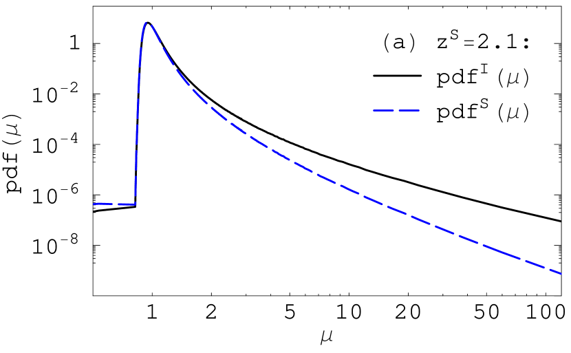
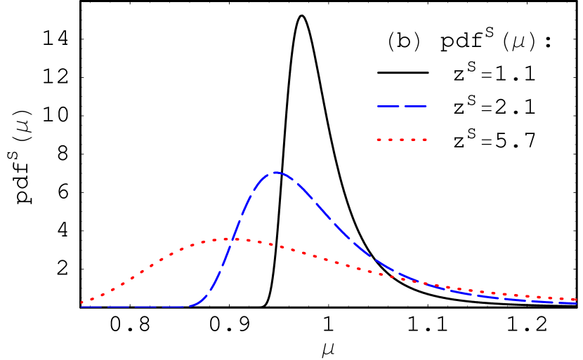
Figure 1: The probability density $\mathrm{pdf}(\mu)$ of the magnification $\mu$. (a) Logarithmic plot comparing $\mathrm{pdf}^{\mathrm{I}}(\mu)$ (solid line) and $\mathrm{pdf}^{\mathrm{S}}(\mu)$ (dashed lines) for a source redshift of $z^{\mathrm{S}}=2.1$. (b) Linear plot comparing the $\mathrm{pdf}^{\mathrm{I}}(\mu)$ around $\mu=1$ for different source redshifts, $z^{\mathrm{S}}=1.1$ (solid line), $z^{\mathrm{S}}=2.1$ (dashed lines) and $z^{\mathrm{S}}=5.7$ (dotted lines).

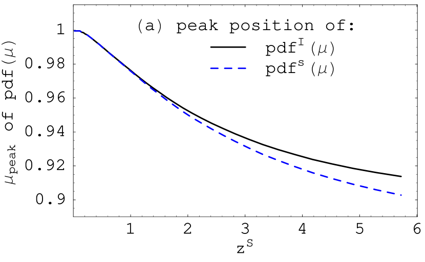
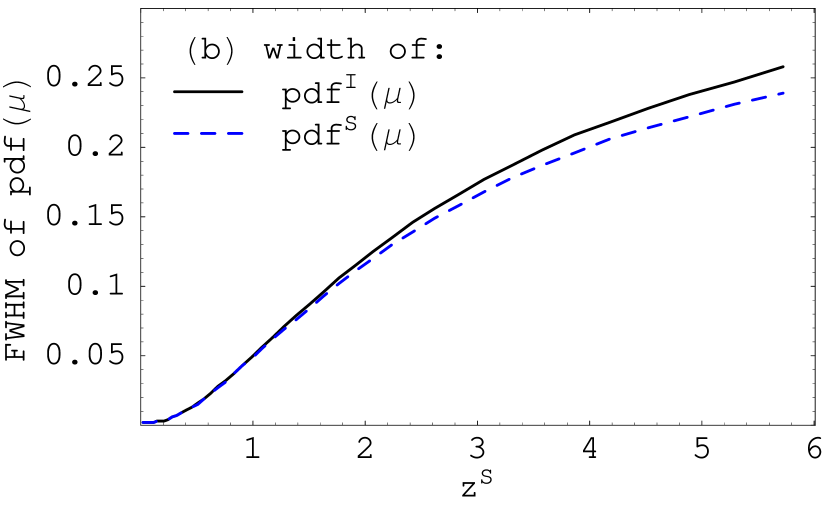
Figure 2: The peak position (a) and the width (b) of the probability densities $\mathrm{pdf}^{\mathrm{I}}(\mu)$ (solid lines) and $\mathrm{pdf}^{\mathrm{S}}(\mu)$ (dashed lines) for the magnification $\mu$ as a function of source redshift $z^{\mathrm{S}}$. The distributions get broader and more skew with increasing $z^{\mathrm{S}}$.

From the magnifications of our random rays, we have estimated the probability density functions $\mathrm{pdf}^{\mathrm{I}}(\mu)$ and $\mathrm{pdf}^{\mathrm{S}}(\mu)$. These are compared for a source redshift $z^{\mathrm{S}}=2.1$ in Fig. 1a. One can readily see the stronger fall-off to high magnification for $\mathrm{pdf}^{\mathrm{S}}(\mu)$, which is a consequence of the relation $\mathrm{pdf}^{\mathrm{S}}(\mu)\approx|\mu|^{-1}\mathrm{pdf}^{\mathrm{I}}(\mu)$ [see Eq. (16) in the Appendix]. The asymptotic behaviour predicted from catastrophe theory (Schneider et al., 1992), i.e. $\mathrm{pdf}^{\mathrm{I}}(\mu)\propto\mu^{-2}$ and $\mathrm{pdf}^{\mathrm{S}}(\mu)\propto\mu^{-3}$, is reached for magnifications $\mu\gtrsim 20$.

Probability density functions $\mathrm{pdf}^{\mathrm{S}}(\mu)$ for different source redshifts $z^{\mathrm{S}}$ are shown in Fig. 1b. With increasing $z^{\mathrm{S}}$, the peak of the distribution broadens and moves to lower $\mu$, whereas the high-$\mu$ tail increases in amplitude. The peak positions and the widths of the pdfs, i.e. their modes $\mu_{\mathrm{peak}}$ and full-widths-at-half-maximum FWHM, are plotted as functions of source redshift in Fig. 2. The shift of the peak with increasing redshift balances the heavier tail so that $\int\mu\mathrm{pdf}^{\mathrm{S}}(\mu)\mathrm{d}{\mu}\,\approx 1$ for all redshifts [see Eq. (17)]. These results for peak position and width are in good agreement with those of Valageas (2000) and Fluke et al. (2002), who considered similar cosmologies.

There is a lower bound to the magnification of images of type I, which is realized for rays which propagate through empty cones (i.e., for which the matter density vanishes along their path) and which are subject to no shear effects (e.g., Dyer & Roeder, 1972; Seitz & Schneider, 1992). No light ray can diverge more strongly than such an empty-beam ray. Lower magnifications can only be produced for overfocussed rays which then belong to Type II or III. A simple way of calculating this lower bound $\mu_{\mathrm{min}}$ for a flat universe is given in Appendix B. The steep rise in the probability density of the magnification at $\mu\approx 0.83$ seen in Fig. 1(a) is substantially larger than the theoretical bound $\mu_{\mathrm{min}}=0.69$ for $z^{\mathrm{S}}=2.1$, indicating that there are no real empty cones in a realistic universe, which is in agreement with findings by Vale & White (2003).

3.2 Strong-lensing optical depths

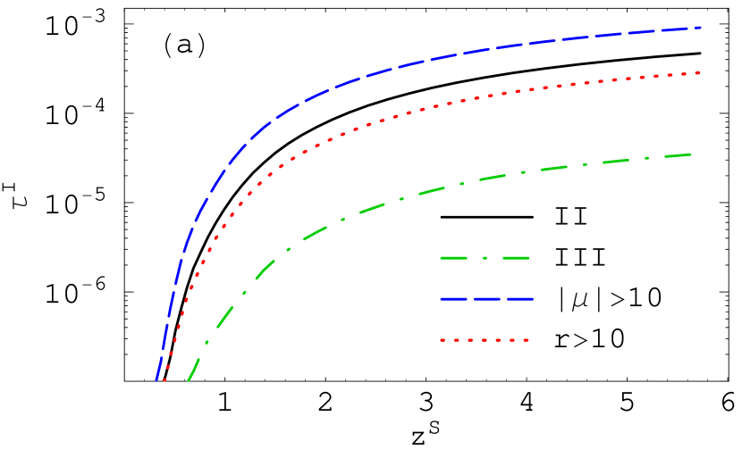
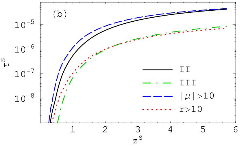
Figure 3: Optical depths for images of small circular sources of type II (solid lines), of type III (dash-dotted lines), with large magnification (dashed lines) and with large length-to-width ratio (dotted lines), assuming a uniform distribution of images in the image plane (a), and a uniform distribution of sources in the source plane (b). Note that the optical depths are significantly smaller in the latter case, and that the relative optical depths for different types of strong lensing are not the same in the two cases.

Sufficiently concentrated matter clumps between distant light sources and the observer can give rise to highly magnified, strongly distorted, or multiple images. We refer to such phenomena as strong lensing. In order to quantify the amount of strong lensing expected in a $\Lambda$CDM universe with the parameters of the Millennium Simulation, we used our large set of random rays to estimate:

• the fraction with $\det\bm{\mathsf{A}}<0$ (type II),

• the fraction with $\det\bm{\mathsf{A}}>0$ and $\mathrm{tr}\,\bm{\mathsf{A}}<0$ (type III),

• the fraction with $\det\bm{\mathsf{A}}<0$ or $\mathrm{tr}\,\bm{\mathsf{A}}<0$, i.e. the sum of the two previous classes (type $\mathrm{II}\vee\mathrm{III}$),

• the fraction with a length-to-width ratio $r>10$ for images of sufficiently small circular sources, and

• the fraction with magnification $|\mu|>10$.

The corresponding optical depths $\tau_{p}^{\mathrm{I}}(z^{\mathrm{S}})$ and $\tau_{p}^{\mathrm{S}}(z^{\mathrm{S}})$ are plotted in Fig. 3 as functions of the source redshift $z^{\mathrm{S}}$. Since all the image properties we consider are (either by definition or at least statistically) associated with large magnifications, the optical depths $\tau_{p}^{\mathrm{S}}(z^{\mathrm{S}})$ are always a factor 5 to 20 smaller than the corresponding $\tau_{p}^{\mathrm{I}}(z^{\mathrm{S}})$.

The optical depths for $r>10$ are 2 to 20 times smaller than those for $|\mu|>10$. Similar results have been found by Dalal et al. (2004) and by Li et al. (2005). Evidently, the optical depth for highly magnified images does not provide a reliable estimate for the probability of images with a large length-to-width ratio.

The optical depth $\tau^{\mathrm{S}}_{r>10}$ may be a reasonable approximation to the optical depth for giant arcs with length-to-width ratio $r>10$, since both finite source size and finite source ellipticity affect this particular property only weakly. Moreover the two effects work in opposite directions. For example, Li et al. (2005) found that the optical depth for ${r>10}$ is almost identical to the optical depth for arc images with length-to-width-ratios $>10$ of elliptical sources with an effective diameter of $1\,\mathrm{arcsec}$.

All our optical depths show a strong dependence on source redshift, similar to that previously noted by Wambsganss et al. (2004) and Li et al. (2005). Comparing to their results in detail, however, we find a somewhat stronger redshift dependence, resulting in 2 to 3 times higher optical depths at $z^{\mathrm{S}}>0.5$. There are various possible explanations for this discrepancy. The simulations they use have 3 to 20 times worse mass resolution than the Millennium Simulation. In addition, Wambsganss et al. (2004) reduced their spatial resolution on lens planes with increasing redshift, thereby potentially missing some low mass lenses, whereas we always use the full spatial resolution permitted by the force resolution of the Millennium Simulation. Furthermore, Wambsganss et al. (2004) measured the fraction of multiply imaged sources for which at least one image has $|\mu|>10$. Thus they do not include sources with a single highly magnified image, as can occur for a marginally subcritical lens. Moreover, they do not account for the fact that multiply imaged sources can give rise to more than one image with $|\mu|>10$. Similarly, Li et al. (2005) only considered the magnification $\mu$ and length-to-width-ratio $r$ of the brightest image of multiply imaged sources for the calculation of the optical depths for ${|\mu|>10}$ and ${r>10}$, although they took into account all giant-arc images for a given population of extended sources in their calculation of the optical depth for giant arcs. Furthermore, they only considered massive clusters and neglected possible contributions from foreground and background matter. These decisions caused them to underestimate the total cross sections for strong lensing (at least for smaller sources).

Fold singularities generically produce strongly magnified and distorted images as pairs, and sources near cusps may give rise to one or three strongly magnified or distorted images (Schneider et al., 1992). Therefore, sources with multiple highly magnified or strongly distorted images might explain a substantial part of the discrepancy between our results and those of Wambsganss et al. (2004) and Li et al. (2005). With our methods, we cannot quantify this effect, but we discuss the other effects further in the following sections.

3.3 Lens properties

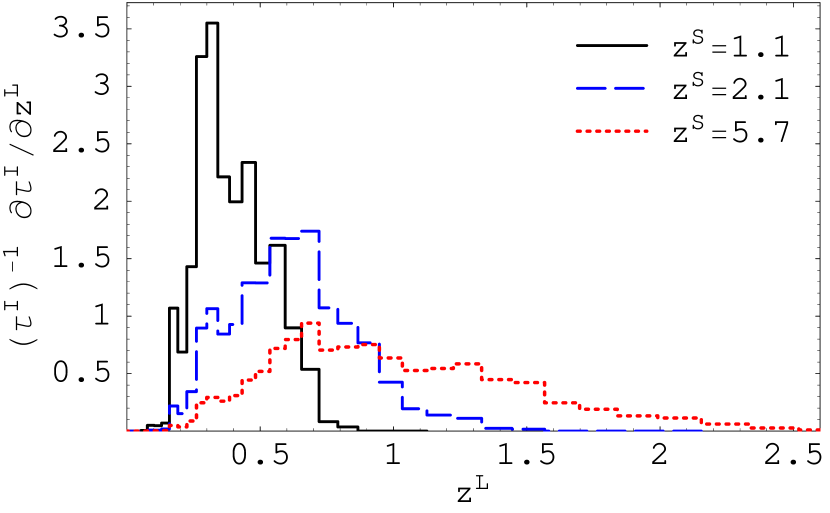
Figure 4: The cross section $\partial\tau^{\mathrm{I}}/\partial z^{\mathrm{L}}$ for rays of type $\mathrm{II}\vee\mathrm{III}$ as a function of lens redshift $z^{\mathrm{L}}$ for sources at redshift $z^{\mathrm{S}}=1.1$ (solid line), $z^{\mathrm{S}}=2.1$ (dashed line), and $z^{\mathrm{S}}=5.7$ (dotted line). Even for high redshift sources, the typical lens redshift is relatively low.

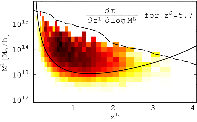
Figure 6: The cross section $\partial\tau^{\mathrm{I}}/\partial z^{\mathrm{L}}\partial\log M^{\mathrm{L}}$ for rays of type $\mathrm{II}\vee\mathrm{III}$ and sources at redshift $z^{\mathrm{S}}=5.7$ as a function of the redshift $z^{\mathrm{L}}$ and halo mass $M^{\mathrm{L}}$ of the lens. Darker areas correspond to higher cross sections (on a logarithmic scale). The dashed line marks the mass of the largest DM halo in the Millennium Simulation at each redshift. The solid line joins masses for which a spherical NFW halo of typical concentration would have Einstein radius $5h^{-1}\,\mathrm{kpc}$, approximately the resolution limit on the lens planes. The cross section for strong lensing in our ray sample is almost entirely contained between these two limits.

In most cases, the properties of strongly lensed rays, i.e. rays with $\det\bm{\mathsf{A}}<0$, $\mathrm{tr}\,\bm{\mathsf{A}}<0$, $|\mu|>10$, or $r>10$, are predominantly caused by a single matter clump along the line of sight. We refer to this as the lens of the ray. In order to find these clumps and to study their properties, we determined for each strongly lensed ray those lens planes which were sufficient to produce the relevant property in the single-plane approximation. Only $2\times 10^{-4}$ of all rays had more than one ‘sufficient’ plane, and we will simply ignore these rays in the following. On the other hand, there was no sufficient plane for up to 41 percent of the rays, depending on source redshift and the property considered, so we will discuss these cases in more detail in Sec 3.4. For most strongly lensed rays, however, this simple criterion identifies exactly one lens plane. The redshift of this plane was then taken as the lens redshift $z^{\mathrm{L}}$ for the ray. For rays of type $\mathrm{II}\vee\mathrm{III}$ (i.e. rays with $\det\bm{\mathsf{A}}<0$ or $\mathrm{tr}\,\bm{\mathsf{A}}<0$), the resulting lens redshift distribution is illustrated in Fig. 4. Here we plot the cross section $\partial\tau^{\mathrm{I}}/\partial z^{\mathrm{L}}$ as a function of lens redshift $z^{\mathrm{L}}$ for various source redshifts $z^{\mathrm{S}}$. Even for sources at redshift $z^{\mathrm{S}}=5.7$, most of the lenses have redshift $z^{\mathrm{L}}<2.5$. The relatively low cross section at higher $z^{\mathrm{L}}$ reflects both the lower abundance of massive halos and the less favourable geometry for lensing at these redshifts (see Fig. 6). The lens redshift distributions for rays with $|\mu|>10$ and with $r>10$ are almost indistinguishable from that of Fig. 4 despite the different total optical depths.

We studied not only the redshift of the clumps acting as strong lenses, but also their masses. All significant matter concentrations have already been identified as DM halos in the simulation and their masses and central positions are available in the simulation archive. We first projected the centres of all halos onto the lens planes in the same way as was done for the particles. For each strongly lensed ray and for all DM halos close to the point where the ray intersects a lens plane, we determined the ratio $M^{\mathrm{L}}/b$, where $M^{\mathrm{L}}$ is the conventional halo mass (defined as the mass within a sphere with mean enclosed density 200 times the cosmological mean), and $b$ denotes the impact parameter of the ray with respect to halo centre.

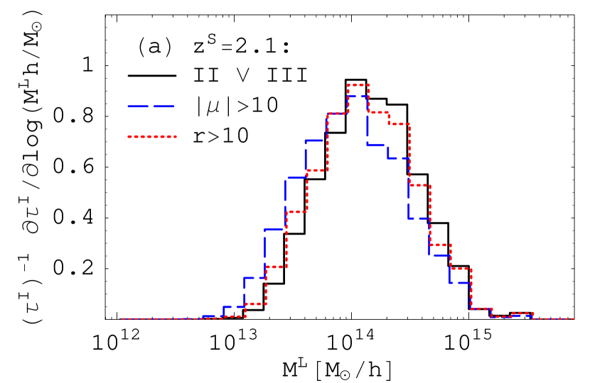
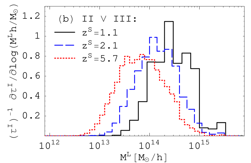
Figure 5: The cross section $\partial\tau^{\mathrm{I}}/\partial\log M^{\mathrm{L}}$ as a function of the mass of the lensing halo $M^{\mathrm{L}}$ (see text). Panel (a) compares rays of type $\mathrm{II}\vee\mathrm{III}$ (solid line), rays with $|\mu|>10$ (dashed line), and rays with $|r|>10$ (dotted line) for source redshift $z^{\mathrm{S}}=2.1$. (b) compares rays of type $\mathrm{II}\vee\mathrm{III}$ for sources at redshift $z^{\mathrm{S}}=1.1$ (solid line), $z^{\mathrm{S}}=2.1$ (dashed line), and $z^{\mathrm{S}}=5.7$ (dotted line). The lens mass distribution is almost independent of the type of strong lensing event, but it shifts towards lower masses for higher source redshift.

The DM halo with the largest $M^{\mathrm{L}}/b$ on the sufficient plane was then defined to be the lens of ray. We discarded from further analysis those 3 to 6 percent of rays for which the largest value of $M^{\mathrm{L}}/b$ was not at least ten times the second largest value. This cut removed all cases where one could not easily separate the influence of several neighbouring DM halos, for example in merging clusters. The resulting distributions of lens masses for rays of type $\mathrm{II}\vee\mathrm{III}$, with $|\mu|>10$, and with $r>10$ are compared in Fig. 5a, where the cross sections $\partial\tau^{\mathrm{I}}/\partial\log M^{\mathrm{L}}$ are plotted for $z^{\mathrm{S}}=2.1$ as a function of lens halo mass $M^{\mathrm{L}}$. Although the corresponding total optical depths are quite different, their lens mass distributions are very similar. There is only a small shift toward lower masses for rays with $|\mu|>10$, and $r>10$ compared to rays of type $\mathrm{II}\vee\mathrm{III}$. In the following we will restrict discussion to the latter for simplicity.

In Fig. 5b, the cross section $\partial\tau^{\mathrm{I}}/\partial\log M^{\mathrm{L}}$ is plotted as a function of mass for type-$\mathrm{II}\vee\mathrm{III}$ rays and for various source redshifts $z^{\mathrm{S}}$. The measured cross section $\partial\tau^{\mathrm{I}}/\partial\log M^{\mathrm{L}}$ vanishes for masses below $4\times 10^{12}h^{-1}\,\mathrm{M}_{\odot}$ and above $4\times 10^{15}h^{-1}\,\mathrm{M}_{\odot}$. The main contribution to the optical depth $\tau^{\mathrm{I}}$ comes from halos with $10^{13}h^{-1}\,\mathrm{M}_{\odot}\lesssim M^{\mathrm{L}}\lesssim 10^{15}h^{-1}\,\mathrm{M}_{\odot}$. For higher source redshifts, the cross section has more weight at lower masses.

The upper mass limit for the cross section simply reflects the fact that there are no halos more massive than $4\times 10^{15}h^{-1}\,\mathrm{M}_{\odot}$ in the simulation. However, the cross section decreases rapidly with increasing $M^{\mathrm{L}}$ already for $M^{\mathrm{L}}>10^{15}h^{-1}\,\mathrm{M}_{\odot}$. The exponential decrease in halo abundance with increasing mass apparently dominates over the increasing cross section of individual halos.

At all source redshifts there is a significant contribution from halos with $M^{\mathrm{L}}<10^{14}h^{-1}\,\mathrm{M}_{\odot}$. For the small sources considered here, the set of DM halos causing strong lensing extends to substantially lower masses than Li et al. (2005) and Dalal et al. (2004) suggest for halos producing giant arcs. The Millennium Simulation has 12 to 20 times better mass resolution than the simulations used by these authors. This provides a considerably better representation of the central halo regions which produce strong lensing. In addition, halos are inefficient in generating strongly distorted images for sources with angular extent comparable to or larger than their Einstein radii. Thus, neglecting or incorrectly treating halos below a given mass (e.g. because of limited mass resolution) has a larger effect on the optical depths for small sources than on those for extended sources – especially for high source redshifts. Together these effects may explain why we find 2 to 3 times larger optical depths at high redshift than the values given by Li et al. (2005).

What sets the lower mass limit for the cross section $\partial\tau^{\mathrm{I}}/\partial\log M^{\mathrm{L}}$? The nominal mass resolution for identifying DM halos in the Millennium Simulation is about $10^{10}h^{-1}\,\mathrm{M}_{\odot}$, so there are plenty of halos with $M^{\mathrm{L}}<4\times 10^{12}h^{-1}\,\mathrm{M}_{\odot}$. The identification limit cannot, in itself, explain the lack of halos less massive than $4\times 10^{12}h^{-1}\,\mathrm{M}_{\odot}$ in our sample. However, the regions capable of causing strong lensing are very small for low-mass halos, so our cross section estimates may be limited by the resolution of our lens planes; critical regions with a diameter below the mesh spacing or the effective gravitational smoothing scale are not resolved. In order to estimate the mass limit induced by these effects, we considered spherical NFW halos (Navarro et al., 1997) with concentration parameter

$$c(M^{\mathrm{L}},z^{\mathrm{L}})=\frac{9.59}{1+z^{\mathrm{L}}}\left(\frac{M^{\mathrm{L}}}{10^{14}h^{-1}\,\mathrm{M}_{\odot}}\right)^{-0.102}$$ (13)

determined by halo mass and redshift (Dolag et al., 2004). For given lens and source redshifts, there is a minimum lens mass for which the Einstein radius exceeds the resolution limit of our lens plane. We take the latter to be $5\,\mathrm{kpc}$ comoving, thus requiring a minimum of four mesh points across the Einstein diameter. This limit takes into account not just the limit imposed by the mesh spacing of $2.5h^{-1}\,\mathrm{kpc}$ ($\sim\!1.7h^{-1}\,\mathrm{kpc}$ in radius), but also the force softening and the smoothing for particles in the halo cores. The solid line in Fig. 6 shows the resulting minimum mass $M^{\mathrm{L}}$ as a function of $z^{\mathrm{L}}$ for $z^{\mathrm{S}}=5.7$. The shading in this plot gives the cross section $\partial^{2}\tau^{\mathrm{I}}/\partial z^{\mathrm{L}}\partial\log M^{\mathrm{L}}$. The region of the $(z^{\mathrm{L}},\log M^{\mathrm{L}})$-plane with non-zero cross section is bounded above by the largest halo mass at each redshift (the dashed line). The lower boundary of this region lies slightly below our analytic estimate of the resolution limit (the solid line). About 6 percent of the cross section is below the analytic estimate. Some deviation is expected because this estimate does not include the effects of intrinsic ellipticity, asymmetries and substructure, and of the scatter in concentration of halos of given mass. It also neglects scatter due to additional matter inhomogeneities along the LOS. These effects should result in strong lensing by somewhat lower mass halos than our simple spherical model would indicate (Meneghetti et al., 2007; Hennawi et al., 2007; Fedeli et al., 2007). In particular, a high-concentration, prolate halo with its major axis along the LOS has a greatly enhanced cross section relative to a spherical halo of the same mass with a typical concentration. Moreover, ellipticity and scatter in concentration lead to larger cross sections on average compared to spherical NFW halos of the mean concentration.

Besides the resolution limit due to the mesh spacing and local smoothing scale on the lens plane, there is another factor limiting the resolution: The critical regions of the relevant halos may not have been simulated to the accuracy required to get fully converged results in the face of discreteness effects resulting from the relatively small number of particles in these regions. According to the criteria given by Power et al. (2003), only the most massive halos in the Millennium Simulation at $0.3<z<2$ should have spherically averaged density profiles which are fully converged at radii comparable to their Einstein radius. At lower masses and at other redshifts the particle number in the inner regions is below the value advocated by Power et al. (2003). (In contrast, the softening length of the Millennium Simulation appears adequate to avoid major problems.) When the particle number is too small, Power et al. (2003) show that simulations typically underestimate the central concentration of a halo, implying a reduction in its strong lensing cross section. This effect is a relatively slow function of particle mass. In addition, strong lensing depends on the projected density distribution rather than the 3-D density profile which Power et al. (2003) studied; there are typically two to three orders of magnitude more particles projected within a halo’s Einstein radius than there are within a central sphere of radius $r_{E}$. Thus it is unclear how seriously the under-resolution of halo cores will affect the cross sections we calculate.

To obtain a rough estimate of how much optical depth we lose due to resolution effects, we calculated the cross section $\partial\tau^{\mathrm{I}}_{\mathrm{II}\vee\mathrm{III}}/\partial\log M^{\mathrm{L}}$ approximating all DM halos in the Millennium Simulation by spherical NFW halos while either (i) taking into account or (ii) disregarding halos with an Einstein radius $r_{\mathrm{E}}<5h^{-1}\,\mathrm{kpc}$ comoving. In doing this, we used the measured maximal circular velocity of each halo to estimate its concentration parameter, rather than assuming the concentration to be given by Eq. (13). The cross sections obtained for the two cases are shown in Fig. 7. Due to the scatter in the halo concentrations, the analytical estimate excluding halos with Einstein radius $r_{E}<5h^{-1}\,\mathrm{kpc}$ extends to lower masses than the limit calculated above by assuming Eq. (13) for all halos. The estimate for $\tau^{\mathrm{I}}_{\mathrm{II}\vee\mathrm{III}}$ including halos with Einstein radius $r_{E}<5h^{-1}\,\mathrm{kpc}$ is only about 15 percent larger than the estimate excluding such halos. Moreover, there is no significant contribution to the full estimate from halos below a few times $10^{12}h^{-1}\,\mathrm{M}_{\odot}$. Indeed, a detailed analysis shows that the strong-lensing cross section of spherical NFW halos with $M^{\mathrm{L}}\leq 10^{13}h^{-1}\,\mathrm{M}_{\odot}$ decreases exponentially with decreasing mass, and is not compensated by the increasing number of halos.

Fig. 7 also shows the two spherical halo-based estimates scaled up by a factor of 3. The curve neglecting halos with small Einstein radii is then a good match to the histogram derived directly from the simulation. Hence, the cross section $\partial\tau^{\mathrm{I}}_{\mathrm{II}\vee\mathrm{III}}/\partial\log M^{\mathrm{L}}$ is about three times as large for simulated halos as for spherical NFW halos, at least for halo masses $M^{\mathrm{L}}>4\times 10^{13}h^{-1}\,\mathrm{M}_{\odot}$ where the resolution limit is unimportant. If this result applies also at lower mass, it implies that limited resolution does not lead us to underestimate total optical depths substantially, perhaps only by about 15%. Note that the missing cross section corresponds to very small image splittings $\Delta\theta^{\mathrm{I}}\lesssim 1\,\mathrm{arcsec}$, a scale where the gravitational effects of the baryons in the central galaxy are expected to be important.

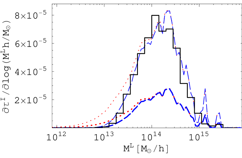
Figure 7: The cross section $\partial\tau^{\mathrm{I}}/\partial\log M^{\mathrm{L}}$ for rays of type $\mathrm{II}\vee\mathrm{III}$ to sources at $z^{\mathrm{S}}=2.1$ as a function of the lensing halo mass $M^{\mathrm{L}}$. The solid histogram gives the direct estimate from the Millennium Simulation. For all other curves we have replaced each halo in the simulation by a spherical NFW halo with the same virial mass and maximal circular velocity. The heavy dotted line gives the result for all halos, while the heavy dashed line shows the effect of excluding all halos with Einstein radius $r_{\mathrm{E}}<5h^{-1}\,\mathrm{kpc}$ comoving. Thin lines show the result of scaling these two curves up by a factor of 3, so that their shape can be compared more easily to the direct estimate from the simulation. The cut-off in cross section at low halo mass in the simulation appears to correspond well to that induced by this simple model for the resolution limit. This suggests that resolution effects reduce our total cross sections by of order 15%.

3.4 Effects of additional matter along the line of sight

For some rays with $\det\bm{\mathsf{A}}<0$, $\mathrm{tr}\,\bm{\mathsf{A}}<0$, $|\mu|>10$, or $r>10$, there is no individual lens plane that is sufficient to produce the relevant property in the single-plane approximation. The fraction of rays for which this is the case is shown in Fig. 8. It increases with increasing source redshift, is lowest for rays of type $\mathrm{II}\vee\mathrm{III}$, and is highest for rays with $r>10$. This fraction gives an indication of the extent to which foreground and background material affects the strong lensing optical depths we have estimated. Such material is expected to have no or little effect on average for the image(s) of a randomly chosen object of given redshift. However, by selecting rays in the extreme tail of lensing distributions, we may be significantly biased towards lines-of-sight for which the additional material enhances the effect of the primary lens. Fig. 8 suggests that additional material is particularly effective in enhancing the probability of highly distorted images (e.g. giant arcs), presumably because these are sensitive to the lensing map in a narrow region around its critical lines. One should, however, bear in mind that not only do certain directions gain a considered property through the primary lens being supplemented by additional LOS material, but other regions lose the same property because the primary lens is counteracted by lower than average additional material. Therefore, the fractions of Fig. 8 do not reflect the overall contribution of line-of-sight material to our cross sections.

In general, the effects of foreground and background material are relatively weak. In the cases where there is no single plane which is sufficient to generate the relevant property, there is still usually a single plane dominating the lensing effects. As an example, we determined for each ray with $|\mu|>10$ and $z^{\mathrm{S}}=5.7$ the planes which gave rise to the largest and second largest magnifications, $\mu_{\text{1st}}$ and $\mu_{\text{2nd}}$, resp., in the single-plane approximation. The cumulative distribution of these magnifications is shown in Fig. 9. Even though the fraction of rays with $\mu_{\text{1st}}<10$ is about 23 percent, virtually all rays have $\mu_{\text{1st}}>2$ and 93 percent of the rays have $\mu_{\text{1st}}>5$. In most of the cases where there is no sufficient lens plane to cause $|\mu|>10$ alone, there is still an ‘almost sufficient’ plane that gives rise to a magnification significantly larger than unity. In only 3 percent of cases is $\mu_{\text{2nd}}>2$, and in 90 percent of all rays we find $\mu_{\text{2nd}}<1.4$. Thus to a good approximation strong lensing can be thought of as being caused by individual objects. These results agree qualitatively with the findings of Wambsganss et al. (2005) for the distribution of the surface mass density.

There are, nevertheless, a few strongly lensed rays whose properties are due to more than one object or lens plane. As noted above, two or more objects at similar redshift contribute significantly for a few percent of all rays. Fig. 9 shows that for a further few percent two or more uncorrelated objects at different redshifts make a significant contribution. For the remaining rays the overall effects of foreground and background matter are at a much lower level. To demonstrate this quantitatively, we first determined the projected mass overdensity at the position of each ray on each plane. We then divided these overdensities by the critical surface densities of the relevant planes. Finally, for each ray we summed the contributions from all planes to obtain a ‘LOS convergence’ $\tilde{\kappa}$, which – to be more precise – is the lensing-efficiency-weighted projection of the matter overdensity along the ray. (This is equal to the convergence $\kappa$ in the single-plane and weak-lensing approximations.) We then performed a similar calculation for all rays of type $\mathrm{II}\vee\mathrm{III}$, with $|\mu|>10$ or with $r>10$. In addition, when calculating $\tilde{\kappa}$ for these rays, we excluded the contribution of the plane containing the primary lens to isolate the contribution $\tilde{\kappa}_{\mathrm{FB}}$ of foreground and background matter to the lensing event. The cumulative distribution of the ratio of $\tilde{\kappa}_{\mathrm{FB}}$ to $\tilde{\kappa}$ is shown in Fig. 10. For 20 percent of the rays of type $\mathrm{II}\vee\mathrm{III}$, additional matter along the LOS contributes more than 10 percent to the total LOS convergence. On the other hand, for 50 percent of the rays, there is a negative contribution $\tilde{\kappa}_{\mathrm{FB}}$. Although there is a noticeable fraction of strongly lensed rays whose LOS convergence is enhanced by additional matter along the LOS, there is also a noticeable fraction of strongly lensed rays whose LOS convergence is decreased due to the lack of matter along the LOS.

In Fig. 11, distributions of the LOS convergence for $z^{\mathrm{S}}=5.7$ are compared for all rays and for strongly lensed rays with the primary lens contribution removed. Although the distributions are very similar, small shifts are visible. In Fig. 12, we show the means of these distributions as a function of source redshift $z^{\mathrm{S}}$. By definition, the mean LOS convergence of all LOS should be zero. The measured mean for our whole ray sample is not exactly zero because of sampling variance, but it is much smaller than the mean for strongly lensed rays with the primary lens excluded. This demonstrates a small but measurable bias towards selecting directions in which matter in front or behind the primary lens enhances the lensing. The effect increases with increasing source redshift, is weakest for the sample of rays with $r>10$, and is strongest for $|\mu|>10$. For $z^{\mathrm{S}}=5.7$ and $|\mu|>10$, where the bias is strongest, we find an average contribution of 0.04 to the LOS convergence. Hence, in all cases the bias is small in comparison with the effect of the primary lens for which $\tilde{\kappa}\sim 1$.

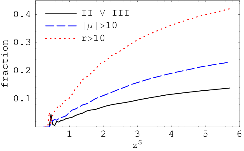
Figure 8: The fraction of rays of type $\mathrm{II}\vee\mathrm{III}$ (solid line), of rays with $|\mu|>10$ (dashed line), and of rays with $r>10$ (dotted line) to source redshift $z^{\mathrm{S}}$ for which no single lens plane is able to generate the relevant property on its own. The relative importance of foreground and background material clearly increases with increasing $z^{\mathrm{S}}$.

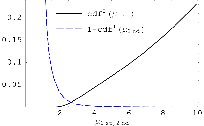
Figure 9: The cumulative distribution function $\mathrm{cdf}^{\mathrm{I}}$ of the largest $\mu_{\text{1st}}$ and of the second largest $\mu_{\text{2nd}}$ single-plane magnification for all rays with a magnification $|\mu|>10$ to source redshift $z^{\mathrm{S}}=5.7$. For clarity we plot $1-\mathrm{cdf}^{\mathrm{I}}(\mu_{\text{2nd}})$ rather than $\mathrm{cdf}^{\mathrm{I}}(\mu_{\text{2nd}})$ so that the high tail of the distribution can be compared with the low tail of $\mathrm{cdf}^{\mathrm{I}}(\mu_{\text{1st}})$. In almost all cases the effect due to the primary lens is strongly dominant.

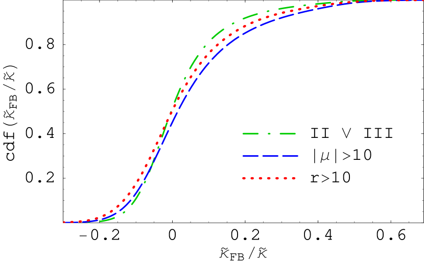
Figure 10: The cumulative distribution function $\mathrm{cdf}(\tilde{\kappa}_{\mathrm{FB}}/\tilde{\kappa})$ of the relative contribution $\tilde{\kappa}_{\mathrm{FB}}/\tilde{\kappa}$ of additional matter to the total LOS convergence $\tilde{\kappa}$ for strongly lensed rays and for source redshift $z^{\mathrm{S}}=5.7$. The dash-dotted line is for rays of type $\mathrm{II}\vee\mathrm{III}$, the dashed line for rays with $|\mu|>10$, and the dotted line for rays with $r>10$.

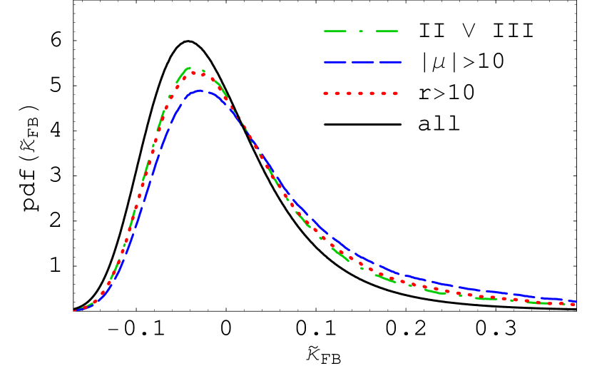
Figure 11: The probability density function $\mathrm{pdf}(\tilde{\kappa}_{\mathrm{FB}})$ of the LOS convergence $\tilde{\kappa}_{\mathrm{BF}}$ for strongly lensed rays and for source redshift $z^{\mathrm{S}}=5.7$, but with the primary lens contribution excluded. The dash-dotted line is for rays of type $\mathrm{II}\vee\mathrm{III}$, the dashed line for rays with $|\mu|>10$, and the dotted line for rays with $r>10$. For comparison, the solid line shows the corresponding distribution $\mathrm{pdf}(\tilde{\kappa})$ for all rays irrespective of their lensing properties. A small but significant shift towards larger convergence is visible in the direction of strong-lensing events.

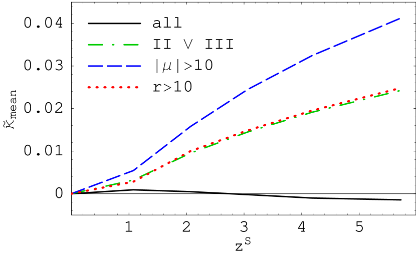
Figure 12: The mean $\tilde{\kappa}_{\mathrm{mean}}$ of the distributions shown in Fig. 11 as a function of source redshift $z^{\mathrm{S}}$. The line types correspond to those of Fig. 11. The mean LOS convergence for all rays irrespective of their lensing properties is non-zero only because of residual sampling variance. The mean convergence from foreground and background matter along rays containing a strong lens is significantly non-zero, however, although still much smaller than the typical convergence due to the primary lens.

4 Summary

The aim of this work has been to study the statistical distribution of the distortion of images of distant sources due to gravitational lensing. In particular, we have concentrated on estimating the cross section for rare strong-lensing events. Our results were obtained by shooting random rays through a series of lens planes created from the Millennium Simulation (Springel et al., 2005). This is the largest $N$-body simulation of cosmological structure formation available today. We have devised improved algorithms to make the lens-planes and to calculate bending angles and shear matrices on these planes in order to take full advantage of the very large volume and the high spatial and mass resolution offered by the simulation.

In Sec. 3.1, we presented results for the statistical distribution of the magnification of point sources. The distribution is skewed with a peak at magnifications below unity and a tail toward high magnification. With increasing source redshift, the peak broadens and moves to lower magnifications, while the tail gains more weight. The magnification distribution affects the observed luminosity distribution of astronomical standard candles. For type Ia supernovae, perhaps the most interesting case, magnification effects on the luminosity distribution are still small for current samples compared to the intrinsic luminosity scatter, to extinction and to other effects. In future high-redshift, high-precision surveys, however, such magnification effects may cause significant systematic errors, so it will be necessary to detect and to correct for them (Dodelson & Vallinotto, 2006; Munshi & Valageas, 2006). In the most optimistic case, detailed comparison with predictions of the magnification distribution may help to discriminate between cosmological models.

Various optical depths connected to strong lensing were presented in Sec. 3.2. In particular, we estimated the fraction of images of sufficiently small sources that are highly magnified, have a large length-to-width ratio, or belong to multiply imaged sources. All the optical depths we analyse increase strongly with increasing redshift. In comparison with earlier results by, e.g., Li et al. (2005) and Wambsganss et al. (2004), we find a stronger evolution with source redshift, leading to higher optical depths for source redshifts $z^{\mathrm{S}}>1$. We discussed possible reasons for this difference.

The results we presented in Sec. 3.3 show that significant contributions to the strong-lensing optical depths come from dark matter halos with masses between $10^{13}h^{-1}\,\mathrm{M}_{\odot}$ and $10^{15}h^{-1}\,\mathrm{M}_{\odot}$. The upper mass limit is due to the very rapidly decreasing abundance of more massive structures. This exponential decrease occurs at lower mass at higher redshift, and in conjunction with the lens geometry it explains why almost all lenses are at redshifts $z^{\mathrm{L}}<2.5$, even for sources with $z^{\mathrm{S}}>5$. The lower mass limit for strong lensing is due primarily to the small cross sections of individual low-mass halos, although the spatial and mass resolution limits of the simulation itself and of our lens planes also play some role. Estimates based on analytic results for spherical NFW halos fit to the Millennium data suggest that these resolution effects are subdominant, and probably only reduce our total cross sections by of order 15%. A more important effect on the relevant scales is our neglect of the baryonic mass of the central galaxies. We will come back to this in later work.

We find that the mass range over which halos can cause strong lensing extends to lower masses than those given by Li et al. (2005) and Dalal et al. (2004). This difference may in part reflect the lower resolution of the simulations used by these authors, and in part the fact that they considered extended sources with diameters $\sim 0.1$–$1\,\mathrm{arcsec}$, while we assumed sufficiently small sources when calculating our cross sections. Halos near our lower mass limit have Einstein radii of order $1\,\mathrm{arcsec}$ and so are inefficient in producing strongly distorted images of sources of comparable angular extent.

Since our set of lens planes represents the whole matter distribution between source and observer, we are able to quantify the influence of foreground and background matter on the frequency and the properties of strong lensing events. We find that such effects are quite modest. On average, the contribution of foreground and background material is only a few percent. Although we do find a bias towards excess foreground and background matter on strong-lensing lines-of-sight, the effect is significantly smaller than suggested by Wambsganss et al. (2005).

The most obvious extension to the work we have presented here would be ray-tracing studies of the effects of lensing for realistic distributions of source properties and across finite size fields. This will, for example, allow direct comparison with observations of massive galaxy clusters where many sets of multiple images are now detected in the best cases (Broadhurst et al., 2005; Halkola et al., 2006). When galaxy properties from galaxy formation modelling within the Millennium Simulation (e.g. Springel et al., 2005; Croton et al., 2006; Bower et al., 2006; De Lucia & Blaizot, 2007) are combined with such ray-tracing analyses, it will be possible to study whether the dark halo masses of individual cluster galaxies are consistent with observation, providing an additional observational test of the hierarchical build-up of structure predicted by the standard $\Lambda$CDM model. This combination of semi-analytic simulation of galaxy formation with ray-tracing measures of lensing will also allow an estimate of how our strong-lensing cross sections should be modified to account for the galaxies, as well as detailed studies of predictions for galaxy-galaxy lensing. We intend to come back to all these topics in future work.

Appendix A Integral relations for the magnification

For a well behaved non-singular lens system, the numbers of images of type I, II and III of a given source satisfy $n_{\mathrm{I}}-n_{\mathrm{II}}+n_{\mathrm{III}}=1$ (Schneider et al., 1992). Here we briefly discuss an ‘integral version’ of this theorem for the particular geometry used in our work: the Multiple-Plane Approximation with lens planes carrying a smooth and non-singular matter distribution that is periodic with a rectangular unit cell of dimensions $L_{1}\times L_{2}$. In this case, the image plane and source plane can both be represented by a rectangle $\mathbb{P}=[0,L_{1}]\times[0,L_{2}]$ with periodic boundary conditions. Furthermore, the lens mapping

$$\mathcal{L}:\mathbb{P}\rightarrow\mathbb{P}:\bm{\theta}\mapsto\bm{\beta}(\bm{\theta})=\bm{\theta}+\bm{\alpha}(\bm{\theta})$$

from image position $\bm{\theta}$ to source position $\bm{\beta}$ for a given source redshift is then smooth and non-singular with a smooth, non-singular, and periodic deflection angle $\bm{\alpha}(\bm{\theta})$. Under these conditions, the inverse signed magnification $\mu^{-1}=\det(\partial\bm{\beta}/\partial\bm{\theta})$ satisfies the following relation:

$$1=\frac{1}{||\mathbb{P}||}\int_{\mathbb{P}}\mathrm{d}^{2}\bm{\theta}\;\mu^{-1}(\bm{\theta}),$$ (14)

where $||\mathbb{P}||=L_{1}L_{2}$ denotes the area of the rectangle $\mathbb{P}$. The following derivation employs integration by parts and exploits the smoothness and periodicity of $(\partial\bm{\beta}/\partial\bm{\theta})$:

$$\begin{split}\int_{\mathbb{P}}\mathrm{d}^{2}\bm{\theta}\;\mu^{-1}(\bm{\theta})&=\int_{\mathbb{P}}\mathrm{d}^{2}\bm{\theta}\;\det\left(\frac{\partial\bm{\beta}}{\partial\bm{\theta}}\right)\\ &=\int_{0}^{L_{1}}\mathrm{d}\theta_{1}\int_{0}^{L_{2}}\mathrm{d}\theta_{2}\;\left(\frac{\partial\beta_{1}}{\partial\theta_{1}}\frac{\partial\beta_{2}}{\partial\theta_{2}}-\frac{\partial\beta_{1}}{\partial\theta_{2}}\frac{\partial\beta_{2}}{\partial\theta_{1}}\right)\\ &=\int_{0}^{L_{2}}\mathrm{d}\theta_{2}\left(\int_{0}^{L_{1}}\mathrm{d}\theta_{1}\;\frac{\partial\beta_{1}}{\partial\theta_{1}}\frac{\partial\beta_{2}}{\partial\theta_{2}}\right)\\ &-\int_{0}^{L_{1}}\mathrm{d}\theta_{1}\left(\int_{0}^{L_{2}}\mathrm{d}\theta_{2}\;\frac{\partial\beta_{1}}{\partial\theta_{2}}\frac{\partial\beta_{2}}{\partial\theta_{1}}\right)\\ &=\int_{0}^{L_{2}}\mathrm{d}\theta_{2}\left(\left[\beta_{1}\frac{\partial\beta_{2}}{\partial\theta_{2}}\right]_{\theta_{1}=0}^{L_{1}}-\int_{0}^{L_{1}}\!\mathrm{d}\theta_{1}\;\beta_{1}\frac{\partial^{2}\beta_{2}}{\partial\theta_{1}\partial\theta_{2}}\right)\\ &-\int_{0}^{L_{1}}\mathrm{d}\theta_{1}\left(\left[\beta_{1}\frac{\partial\beta_{2}}{\partial\theta_{1}}\right]_{\theta_{2}=0}^{L_{2}}-\int_{0}^{L_{2}}\!\mathrm{d}\theta_{2}\;\beta_{1}\frac{\partial^{2}\beta_{2}}{\partial\theta_{1}\partial\theta_{2}}\right)\\ &=\int_{0}^{L_{2}}\mathrm{d}\theta_{2}\left[\beta_{1}\frac{\partial\beta_{2}}{\partial\theta_{2}}\right]_{\theta_{1}=0}^{L_{1}}-\int_{0}^{L_{1}}\mathrm{d}\theta_{1}\left[\beta_{1}\frac{\partial\beta_{2}}{\partial\theta_{1}}\right]_{\theta_{2}=0}^{L_{2}}\\ &=\int_{0}^{L_{2}}\mathrm{d}\theta_{2}\left[\beta_{1}(L_{1},\theta_{2})-\beta_{1}(0,\theta_{2})\right]\frac{\partial\beta_{2}(L_{1},\theta_{2})}{\partial\theta_{2}}\\ &-\int_{0}^{L_{1}}\mathrm{d}\theta_{1}\left[\beta_{1}(\theta_{1},L_{2})-\beta_{1}(\theta_{1},0)\right]\frac{\partial\beta_{2}(\theta_{1},L_{2})}{\partial\theta_{2}}\\ &=\int_{0}^{L_{2}}\mathrm{d}\theta_{2}L_{1}\frac{\partial\beta_{2}(L_{1},\theta_{2})}{\partial\theta_{2}}\\ &=L_{1}L_{2}\;.\end{split}$$

For our ray sampling method, it follows directly from relation (14) that a representative sample of rays with random positions $\bm{\theta}_{i}$ ($i=1,\ldots,N$) in the image plane should satisfy:

$$\frac{1}{N}\sum_{i=1}^{N}\mu^{-1}(\bm{\theta}_{i})\approx\frac{1}{||\mathbb{P}||}\int_{\mathbb{P}}\mathrm{d}^{2}\bm{\theta}\;\mu^{-1}(\bm{\theta})=1.$$ (15)

For our ray sample, we find that

$$\left|\frac{1}{N}\sum_{i=1}^{N}\mu^{-1}(\bm{\theta}_{i})\right|-1<0.003$$

for all source redshifts.

For the magnification distribution, Eq. (14) implies that

$$\begin{split}\mathrm{pdf}^{\mathrm{S}}(\mu^{\prime})&=\frac{\mathrm{d}}{\mathrm{d}\mu^{\prime}}\frac{\int_{\mathbb{P}}\mathrm{d}^{2}{\bm{\theta}}\,\left|\mu(\bm{\theta})\right|^{-1}\Theta[\mu^{\prime}-\mu(\bm{\theta})]}{\int_{\mathbb{P}}\mathrm{d}^{2}{\bm{\theta}}\,\left|\mu(\bm{\theta})\right|^{-1}}\\ &=\frac{\int_{\mathbb{P}}\mathrm{d}^{2}{\bm{\theta}}\,\left|\mu(\bm{\theta})\right|^{-1}\delta[\mu^{\prime}-\mu(\bm{\theta})]}{\int_{\mathbb{P}}\mathrm{d}^{2}{\bm{\theta}}\,\left|\mu(\bm{\theta})\right|^{-1}}\\ &=|\mu^{\prime}|^{-1}\frac{\int_{\mathbb{P}}\mathrm{d}^{2}{\bm{\theta}}\,\delta[\mu^{\prime}-\mu(\bm{\theta})]}{\int_{\mathbb{P}}\mathrm{d}^{2}{\bm{\theta}}\,\left|\mu(\bm{\theta})\right|^{-1}}\\ &=\frac{\int_{\mathbb{P}}\mathrm{d}^{2}{\bm{\theta}}\,}{\int_{\mathbb{P}}\mathrm{d}^{2}{\bm{\theta}}\,\left|\mu(\bm{\theta})\right|^{-1}}|\mu^{\prime}|^{-1}\mathrm{pdf}^{\mathrm{I}}(\mu^{\prime})\\ &=\left(1-2\,\tau^{\mathrm{S}}_{\mathrm{II}}\right)|\mu^{\prime}|^{-1}\mathrm{pdf}^{\mathrm{I}}(\mu^{\prime})\;.\end{split}$$

In practice, the optical depth $\tau^{\mathrm{S}}_{\mathrm{II}}$ for images with negative magnification is very small. Hence,

$$\begin{split}\mathrm{pdf}^{\mathrm{S}}(\mu^{\prime})&\approx|\mu^{\prime}|^{-1}\mathrm{pdf}^{\mathrm{I}}(\mu^{\prime}).\end{split}$$ (16)

Employing the fact that both probability distributions are normalised, we finally find:

$$\int_{\mathbb{R}}\left|\mu\right|^{-1}\mathrm{pdf}^{\mathrm{I}}(\mu)\,\mathrm{d}{\mu}\,\approx 1\;,\;\text{ and}\;\;\;\int_{\mathbb{R}}\left|\mu\right|\mathrm{pdf}^{\mathrm{S}}(\mu)\,\mathrm{d}{\mu}\,\approx 1.$$ (17)

Appendix B Empty-beam magnification in a flat universe

The Jacobian of the lens mapping for light propagation through an inhomogeneous universe is given by (see, e.g., Schneider, 2006a):

$$\bm{\mathsf{A}}_{ij}(\bm{\theta},w)=\delta_{ij}\\ -\frac{2}{c^{2}}\int_{0}^{w}\!\!\mathrm{d}{w^{\prime}}\,\frac{(w-w^{\prime})w^{\prime}}{w}\frac{\partial^{2}\Phi(\bm{x}(\bm{\theta},w^{\prime}),w^{\prime})}{\partial\theta_{i}\,\partial\theta_{k}}\,\bm{\mathsf{A}}_{kj}(\bm{\theta},w^{\prime}).$$ (18)

Here, $\Phi$ denotes the three-dimensional gravitational potential, $w$ the comoving line-of-sight distance and $\bm{\theta}$ the direction of the light ray, and $\bm{x}$ the comoving transverse separation. For an empty beam, we have $\bm{\mathsf{A}}={\rm diag}(\mu_{\mathrm{min}}^{-1/2},\mu_{\mathrm{min}}^{-1/2})$. Furthermore, the Poisson equation in this case reads

$$\nabla^{2}\Phi(\bm{x}(\bm{\theta},w),w)=-\frac{3H_{0}^{2}\Omega_{\rm m}}{2a(w)}\;,$$

where $a(w)$ is the scale factor.

Considering now the $1,1$-component of Eq. (18), we find

$$\mu_{\mathrm{min}}^{-1/2}(w)=1+\frac{3H_{0}^{2}\Omega_{\rm m}}{2c^{2}}\int_{0}^{w}\!\mathrm{d}{w^{\prime}}\,\frac{(w-w^{\prime})w^{\prime}}{a(w^{\prime})w}\,\mu_{\mathrm{min}}^{-1/2}(w^{\prime})\;.$$

Differentiating this expression twice, we finally obtain the differential equation

$$\frac{\mathrm{d}^{2}{f}\,}{\mathrm{d}{w^{2}}\,}=\frac{3H_{0}^{2}\Omega_{\rm m}}{2c^{2}}\,\frac{f(w)}{a(w)}\;,$$

where $f(w)\equiv w\mu_{\mathrm{min}}^{-1/2}(w)$. This ordinary differential equation can be easily solved numerically.

References

- Amanullah et al. (2003) Amanullah, R., Mörtsell, E., & Goobar, A. 2003, A&A, 397, 819
- Barris et al. (2004) Barris, B. J., Tonry, J. L., Blondin, S., et al. 2004, ApJ, 602, 571
- Bartelmann et al. (1998) Bartelmann, M., Huss, A., Colberg, J. M., Jenkins, A., & Pearce, F. R. 1998, A&A, 330, 1
- Blandford & Narayan (1986) Blandford, R. & Narayan, R. 1986, ApJ, 310, 568
- Bower et al. (2006) Bower, R. G., Benson, A. J., Malbon, R., et al. 2006, MNRAS, 370, 645
- Broadhurst et al. (2005) Broadhurst, T., Benítez, N., Coe, D., et al. 2005, ApJ, 621, 53
- Comerford et al. (2006) Comerford, J. M., Meneghetti, M., Bartelmann, M., & Schirmer, M. 2006, ApJ, 642, 39
- Cooley & Tukey (1965) Cooley, J. W. & Tukey, J. W. 1965, Math. Comput., 19, 297
- Croton et al. (2006) Croton, D. J., Springel, V., White, S. D. M., et al. 2006, MNRAS, 365, 11
- Dalal et al. (2004) Dalal, N., Holder, G., & Hennawi, J. F. 2004, ApJ, 609, 50
- De Lucia & Blaizot (2007) De Lucia, G. & Blaizot, J. 2007, MNRAS, 375, 2
- Dodelson & Vallinotto (2006) Dodelson, S. & Vallinotto, A. 2006, Phys. Rev. D, 74, 063515
- Dolag et al. (2004) Dolag, K., Bartelmann, M., Perrotta, F., et al. 2004, A&A, 416, 853
- Dyer & Roeder (1972) Dyer, C. C. & Roeder, R. C. 1972, ApJ, 174, L115
- Fedeli et al. (2007) Fedeli, C., Bartelmann, M., Meneghetti, M., & Moscardini, L. 2007, ArXiv e-prints, 705
- Fluke et al. (2002) Fluke, C. J., Webster, R. L., & Mortlock, D. J. 2002, MNRAS, 331, 180
- Frigo & Johnson (2005) Frigo, M. & Johnson, S. G. 2005, Proc. IEEE, 93, 216
- Gladders et al. (2003) Gladders, M. D., Hoekstra, H., Yee, H. K. C., Hall, P. B., & Barrientos, L. F. 2003, ApJ, 593, 48
- Halkola et al. (2006) Halkola, A., Seitz, S., & Pannella, M. 2006, MNRAS, 372, 1425
- Hennawi et al. (2007) Hennawi, J. F., Dalal, N., Bode, P., & Ostriker, J. P. 2007, ApJ, 654, 714
- Hetterscheidt et al. (2007) Hetterscheidt, M., Simon, P., Schirmer, M., et al. 2007, A&A, 468, 859
- Hewitt et al. (1988) Hewitt, J. N., Turner, E. L., Schneider, D. P., Burke, B. F., & Langston, G. I. 1988, Nature, 333, 537
- Hilbert et al. (2007) Hilbert, S., Hartlap, J., White, S. D. M., & Schneider, P. 2007, in preparation
- Hoekstra et al. (2006) Hoekstra, H., Mellier, Y., van Waerbeke, L., et al. 2006, ApJ, 647, 116
- Hoekstra et al. (2002) Hoekstra, H., van Waerbeke, L., Gladders, M. D., Mellier, Y., & Yee, H. K. C. 2002, ApJ, 577, 604
- Holz (1998) Holz, D. E. 1998, ApJ, 506, L1
- Horesh et al. (2005) Horesh, A., Ofek, E. O., Maoz, D., et al. 2005, ApJ, 633, 768
- Jain et al. (2000) Jain, B., Seljak, U., & White, S. 2000, ApJ, 530, 547
- Jönsson et al. (2006) Jönsson, J., Dahlén, T., Goobar, A., et al. 2006, ApJ, 639, 991
- Knop et al. (2003) Knop, R. A., Aldering, G., Amanullah, R., et al. 2003, ApJ, 598, 102
- Kochanek (2006) Kochanek, C. S. 2006, in Saas-Fee Advanced Course 33: Gravitational Lensing: Strong, Weak and Micro, ed. G. Meylan, P. Jetzer, P. North, P. Schneider, C. S. Kochanek, & J. Wambsganss, 91–268
- Li et al. (2005) Li, G.-L., Mao, S., Jing, Y. P., et al. 2005, ApJ, 635, 795
- Li et al. (2006) Li, G. L., Mao, S., Jing, Y. P., et al. 2006, MNRAS, 372, L73
- Luppino et al. (1999) Luppino, G. A., Gioia, I. M., Hammer, F., Le Fèvre, O., & Annis, J. A. 1999, A&AS, 136, 117
- Lynds & Petrosian (1986) Lynds, R. & Petrosian, V. 1986, in Bulletin of the American Astronomical Society, 1014
- Mandelbaum et al. (2006a) Mandelbaum, R., Seljak, U., Cool, R. J., et al. 2006a, MNRAS, 372, 758
- Mandelbaum et al. (2006b) Mandelbaum, R., Seljak, U., Kauffmann, G., Hirata, C. M., & Brinkmann, J. 2006b, MNRAS, 368, 715
- Massey et al. (2007) Massey, R., Rhodes, J., Leauthaud, A., et al. 2007, ArXiv Astrophysics e-prints
- Meneghetti et al. (2007) Meneghetti, M., Argazzi, R., Pace, F., et al. 2007, A&A, 461, 25
- Meneghetti et al. (2000) Meneghetti, M., Bolzonella, M., Bartelmann, M., Moscardini, L., & Tormen, G. 2000, MNRAS, 314, 338
- Metcalf (1999) Metcalf, R. B. 1999, MNRAS, 305, 746
- Metcalf & Silk (1999) Metcalf, R. B. & Silk, J. 1999, ApJ, 519, L1
- Minty et al. (2002) Minty, E. M., Heavens, A. F., & Hawkins, M. R. S. 2002, MNRAS, 330, 378
- Munshi & Valageas (2006) Munshi, D. & Valageas, P. 2006, ArXiv Astrophysics e-prints
- Narayan & White (1988) Narayan, R. & White, S. D. M. 1988, MNRAS, 231, 97P
- Natarajan et al. (2007) Natarajan, P., De Lucia, G., & Springel, V. 2007, MNRAS, 376, 180
- Navarro et al. (1997) Navarro, J. F., Frenk, C. S., & White, S. D. M. 1997, ApJ, 490, 493
- Oguri et al. (2003) Oguri, M., Lee, J., & Suto, Y. 2003, ApJ, 599, 7
- Power et al. (2003) Power, C., Navarro, J. F., Jenkins, A., et al. 2003, MNRAS, 338, 14
- Riess et al. (1998) Riess, A. G., Filippenko, A. V., Challis, P., et al. 1998, AJ, 116, 1009
- Riess et al. (2004) Riess, A. G., Strolger, L.-G., Tonry, J., et al. 2004, ApJ, 607, 665
- Schneider (2006a) Schneider, P. 2006a, in Saas-Fee Advanced Course 33: Gravitational Lensing: Strong, Weak and Micro, ed. G. Meylan, P. Jetzer, P. North, P. Schneider, C. S. Kochanek, & J. Wambsganss, 1–89
- Schneider (2006b) Schneider, P. 2006b, in Saas-Fee Advanced Course 33: Gravitational Lensing: Strong, Weak and Micro, ed. G. Meylan, P. Jetzer, P. North, P. Schneider, C. S. Kochanek, & J. Wambsganss, 269–451
- Schneider et al. (1992) Schneider, P., Ehlers, J., & Falco, E. E. 1992, Gravitational Lenses (Springer-Verlag)
- Seitz & Schneider (1992) Seitz, S. & Schneider, P. 1992, A&A, 265, 1
- Seljak et al. (2005) Seljak, U., Makarov, A., Mandelbaum, R., et al. 2005, Phys. Rev. D, 71, 043511
- Semboloni et al. (2006) Semboloni, E., Mellier, Y., van Waerbeke, L., et al. 2006, A&A, 452, 51
- Simon et al. (2007) Simon, P., Hetterscheidt, M., Schirmer, M., et al. 2007, A&A, 461, 861
- Soucail et al. (1987) Soucail, G., Mellier, Y., Fort, B., Mathez, G., & Hammer, F. 1987, A&A, 184, L7
- Spergel et al. (2007) Spergel, D. N., Bean, R., Doré, O., et al. 2007, ApJS, 170, 377
- Springel (2005) Springel, V. 2005, MNRAS, 364, 1105
- Springel et al. (2005) Springel, V., White, S. D. M., Jenkins, A., et al. 2005, Nature, 435, 629
- Subramanian et al. (1987) Subramanian, K., Rees, M. J., & Chitre, S. M. 1987, MNRAS, 224, 283
- Turner et al. (1984) Turner, E. L., Ostriker, J. P., & Gott, III, J. R. 1984, ApJ, 284, 1
- Tyson et al. (1990) Tyson, J. A., Wenk, R. A., & Valdes, F. 1990, ApJ, 349, L1
- Valageas (2000) Valageas, P. 2000, A&A, 354, 767
- Vale & White (2003) Vale, C. & White, M. 2003, ApJ, 592, 699
- Walsh et al. (1979) Walsh, D., Carswell, R. F., & Weymann, R. J. 1979, Nature, 279, 381
- Wambsganss et al. (2004) Wambsganss, J., Bode, P., & Ostriker, J. P. 2004, ApJ, 606, L93
- Wambsganss et al. (2005) Wambsganss, J., Bode, P., & Ostriker, J. P. 2005, ApJ, 635, L1
- Wambsganss et al. (1997) Wambsganss, J., Cen, R., Xu, G., & Ostriker, J. P. 1997, ApJ, 475, L81
- Wang (2005) Wang, Y. 2005, Journal of Cosmology and Astroparticle Physics, 2005, 005
- Wu & Chiueh (2006) Wu, J. M. & Chiueh, T. 2006, ApJ, 639, 695
- Zaritsky & Gonzalez (2003) Zaritsky, D. & Gonzalez, A. H. 2003, ApJ, 584, 691