Analysis of Collective Neutrino Flavor Transformation in Supernovae

Abstract

We study the flavor evolution of a dense gas initially consisting of pure mono-energetic $\nu_{e}$ and $\bar{\nu}_{e}$. Using adiabatic invariants and the special symmetry in such a system we are able to calculate the flavor evolution of the neutrino gas for the cases with slowly decreasing neutrino number densities. These calculations give new insights into the results of recent large-scale numerical simulations of neutrino flavor transformation in supernovae. For example, our calculations reveal the existence of what we term the “collective precession mode”. Our analyses suggest that neutrinos which travel on intersecting trajectories subject to destructive quantum interference nevertheless can be in this mode. This mode can result in sharp transitions in the final energy-dependent neutrino survival probabilities across all trajectories, a feature seen in the numerical simulations. Moreover, this transition is qualitatively different for the normal and inverted neutrino mass hierarchies. Exploiting this difference, the neutrino signals from a future galactic supernova can potentially be used to determine the actual neutrino mass hierarchy.

I Introduction

In this paper we employ physical, analytic insights along with the results of large-scale numerical calculations to study the nature of collective neutrino and antineutrino flavor transformation in supernovae. Although neutrino flavor transformation is an experimental fact, modeling this process in astrophysical settings can be problematic. In part, this is because nature produces environments where the number densities of neutrinos and/or antineutrinos can be very large. Examples of these include the early universe and environments associated with compact-object mergers and gravitational collapse. In particular, core-collapse supernovae result in hot proto-neutron stars that emit neutrinos and antineutrinos copiously from the neutrino sphere. This implies inhomogeneous, anisotropic distributions for these particles. As their trajectories intersect above the proto-neutron star, their flavor evolution histories are quantum mechanically coupled Qian and Fuller (1995). The flavor content of the neutrino and antineutrino fields in and above a proto-neutron star will be a necessary ingredient for the interpretation of neutrino signals from a future supernova. It can also be an important, even crucial determinant of the composition of supernova ejecta Qian et al. (1993) and possibly even the supernova explosion mechanism Fuller et al. (1992). Consequently, if we are to understand core-collapse supernovae, it follows that we must understand neutrino and antineutrino flavor evolution in them.

Large neutrino number densities imply that neutrino-neutrino in addition to neutrino-electron forward scattering sets the potential which governs neutrino flavor conversion. Because of the neutrino-neutrino forward scattering potential Fuller et al. (1987); Pantaleone (1992); Sigl and Raffelt (1993), neutrino flavor transformation in the early universe and near the supernova core can be very different from that in the vacuum or in an ordinary matter background only Samuel (1993); Kostelecky and Samuel (1994); Kostelecky et al. (1993); Kostelecky and Samuel (1993, 1995); Samuel (1996); Kostelecky and Samuel (1996); Pastor et al. (2002); Dolgov et al. (2002); Wong (2002); Abazajian et al. (2002). Recent analytical and numerical studies have revealed a new paradigm for neutrino flavor transformation in supernovae Pastor and Raffelt (2002); Balantekin and Yüksel (2005); Fuller and Qian (2006); Duan et al. (2005, 2006a, 2006b); Hannestad et al. (2006); Balantekin and Pehlivan (2007); Raffelt and Sigl (2007), one which is completely different from vacuum oscillations or the conventional Mikheyev-Smirnov-Wolfenstein (MSW) mechanism Wolfenstein (1978, 1979); Mikheyev and Smirnov (1985).

A particular aspect of this new paradigm is best discussed in the following framework: The $2\times 2$ neutrino flavor transformation problem can be described as the motion of isospins in flavor space, wherein $\nu_{e}/\bar{\nu}_{\mu,\tau}$ and $\bar{\nu}_{e}/\nu_{\mu,\tau}$ correspond to the “up” and “down” states of these isospins Duan et al. (2005). Both analytical and numerical studies have suggested that a dense neutrino gas originally in a “bipolar configuration” (i.e., with the corresponding neutrino flavor isospins or NFIS’s forming two oppositely oriented groups) tends to stay in such a configuration even though each isospin group is composed of neutrinos and/or antineutrinos with finite energy spread. In other words, neutrinos and antineutrinos with different energies can experience collective flavor transformation at high neutrino number densities. This is very different from the conventional MSW paradigm in which neutrinos and antineutrinos with different energies undergo flavor transformation independently.

A neutrino system with a bipolar configuration is also referred to as a “bipolar system”. Because supernova neutrinos are essentially in their flavor eigenstates when they leave the neutrino sphere, they naturally form a bipolar system. The neutrino sphere is in the very high density, electron degenerate environment near the neutron star surface.

For a simple bipolar system consisting of mono-energetic $\nu_{e}$ and $\bar{\nu}_{e}$ initially, it has been shown that the evolution of the system is equivalent to the motion of a (gyroscopic) pendulum Hannestad et al. (2006). Therefore, a bipolar system generally can evolve simultaneously in two different kinds of modes, i.e. the precession mode and the nutation mode, in analogy to the mechanical motion of a gyroscopic pendulum. In the extreme limit of large neutrino number density, a bipolar system is reduced to a synchronized system, which is in a pure precession mode characterized by a common synchronization frequency Pastor et al. (2002). The evolution of bipolar systems in the presence of an ordinary matter background has been studied in Refs. Duan et al. (2005); Hannestad et al. (2006) using corotating frames.

Refs. Duan et al. (2006a, b) have presented by far the most sophisticated, large-scale numerical simulations of neutrino flavor transformation in the coherent regime near the supernova core. For example, these simulations for the first time self-consistently treated the evolution of neutrinos propagating along various intersecting trajectories. These simulations clearly show that the conventional MSW paradigm is invalid near the supernova core where neutrino fluxes are large. However, analytical models so far have only corroborated some of the features demonstrated by the simulations, and there are some obvious gaps between the analytical and numerical studies.

One of the gaps is that current analytical models of bipolar systems assume constant neutrino number densities, which is not true in supernovae. Using some simple numerical examples, Ref. Hannestad et al. (2006) has shown that some interesting phenomena observed in the simulations Duan et al. (2006a, b) are related to varying neutrino number densities. For example, the energy averaged neutrino survival probabilities change as neutrino number densities decrease with the radius. In this paper we will show that if the neutrino number density decreases slowly as the system evolves out of the synchronized limit at high neutrino densities, the bipolar system will be dominantly in a precession mode. The neutrino flavor evolution seen in the numerical simulations is the combined effect of this precession mode and the nutation modes that are generated as a result of the finite rate of change in neutrino number densities.

Another important gap between analytical and numerical studies is that most of the current analytical models assume homogeneity and isotropy of the neutrino gas, which is not true of the supernova environment. A recent analytical study which assumes an initial state of $\nu_{e}$ and $\bar{\nu}_{e}$ with equal densities shows that the collectivity (referred to as “coherence” or “kinematic coherence” in Ref. Hannestad et al. (2006)) of the nutation modes tends to break down quickly among different neutrino trajectories in an inhomogeneous and anisotropic environment Raffelt and Sigl (2007). However, the numerical simulations presented in Refs. Duan et al. (2006a, b) employed more realistic supernova conditions where the initial $\nu_{e}$ and $\bar{\nu}_{e}$ as well as $\nu_{\mu,\tau}$ and $\bar{\nu}_{\mu,\tau}$ do not have the same number densities. These simulations do show some clear signs of collective flavor transformation. One important example is the hallmark pattern in the final energy-dependent neutrino survival probability which has a sharp transition energy across all neutrino trajectories (Fig. 3 of Ref. Duan et al. (2006b)). We have further analyzed the numerical results obtained in the large-scale simulations mentioned above and found that, apart from the non-collective nutation modes, neutrinos propagating along different trajectories were in a single, collective precession mode. It is this precession mode that facilitates the mechanism suggested in Ref. Duan et al. (2006a) for producing the fore-mentioned hallmark pattern in the final neutrino survival probability.

This paper is organized as follows. In Sec. II we will study the properties of a symmetric bipolar system initially consisting of an equal number of $\nu_{e}$ and $\bar{\nu}_{e}$. We will use an adiabatic invariant of the system to obtain some analytical understanding of the evolution of such a system as neutrino number densities change. In Sec. III we will compare a simple asymmetric bipolar system with a gyroscopic pendulum. We will revisit the criteria determining whether a bipolar system is in the synchronized or bipolar regime and clarify the description of bipolar oscillations. In Sec. IV we will show that an asymmetric bipolar system can stay roughly in a pure precession mode if neutrino number densities decrease slowly. We will also demonstrate some interesting properties of such a precession mode which can explain the results from the simple numerical examples of Ref. Hannestad et al. (2006). In Sec. V we will apply our simple analytical models to understand the numerical simulations presented in Refs. Duan et al. (2006a, b) and offer some new analyses of these simulations. In Sec. VI we give our conclusions.

II Symmetric Bipolar System

II.1 Flavor pendulum

We start with a simple bipolar system initially consisting of mono-energetic $\nu_{e}$ and $\bar{\nu}_{e}$ with energy $E_{\nu}$ and an equal number density $n_{\nu}$. Throughout this paper we will assume $2\times 2$ flavor mixing through the active-active channel. According to Ref. Duan et al. (2005), the flavor evolution of a neutrino or antineutrino is equivalent to the motion of the corresponding neutrino flavor isospin, or NFIS, in flavor space. For a neutrino, the NFIS in the flavor basis is defined as

$$\mathbf{s}_{\nu}\equiv\frac{1}{2}\begin{pmatrix}2\mathrm{Re}(a_{\nu_{e}}^{*}a_{\nu_{\tau}})\\ 2\mathrm{Im}(a_{\nu_{e}}^{*}a_{\nu_{\tau}})\\ |a_{\nu_{e}}|^{2}-|a_{\nu_{\tau}}|^{2}\end{pmatrix},$$ (1)

where $a_{\nu_{e}}$ and $a_{\nu_{\tau}}$ are the amplitudes for the neutrino to be in $\nu_{e}$ and another flavor state, say $\nu_{\tau}$, respectively. For an antineutrino, the corresponding NFIS in the flavor basis is

$$\mathbf{s}_{\bar{\nu}}\equiv-\frac{1}{2}\begin{pmatrix}2\mathrm{Re}(a_{\bar{\nu}_{e}}a_{\bar{\nu}_{\tau}}^{*})\\ 2\mathrm{Im}(a_{\bar{\nu}_{e}}a_{\bar{\nu}_{\tau}}^{*})\\ |a_{\bar{\nu}_{e}}|^{2}-|a_{\bar{\nu}_{\tau}}|^{2}\end{pmatrix},$$ (2)

where $a_{\bar{\nu}_{e}}$ and $a_{\bar{\nu}_{\tau}}$ are the amplitudes for the antineutrino to be $\bar{\nu}_{e}$ and $\bar{\nu}_{\tau}$, respectively.

To obtain a simple analytical understanding of collective neutrino flavor transformation, we will assume, unless otherwise stated, that the neutrino gas is homogeneous and isotropic and that there is no ordinary matter medium. Using the NFIS notation, the equations of motion (e.o.m.) for the NFIS’s $\mathbf{s}_{1}$ (neutrino) and $\mathbf{s}_{2}$ (antineutrino) of this simple bipolar system are Duan et al. (2005)

$$\frac{\mathrm{d}}{\mathrm{d}t}\mathbf{s}_{1} =\mathbf{s}_{1}\times(\mu_{\mathrm{V},1}\mathbf{H}_{\mathrm{V}}+\mu_{\nu}n_{\nu,2}\mathbf{s}_{2}),$$ (3a)

$$\frac{\mathrm{d}}{\mathrm{d}t}\mathbf{s}_{2} =\mathbf{s}_{2}\times(\mu_{\mathrm{V},2}\mathbf{H}_{\mathrm{V}}+\mu_{\nu}n_{\nu,1}\mathbf{s}_{1}),$$ (3b)

and the initial condition is

$$\mathbf{s}_{1}(0)=-\mathbf{s}_{2}(0)=\frac{\bm{\hat{\mathbf{e}}}^{\mathrm{f}}_{z}}{2},$$ (4)

where

$$n_{\nu,1}=n_{\nu,2}=n_{\nu}$$ (5)

are the number densities of neutrinos and antineutrinos, and $\bm{\hat{\mathbf{e}}}^{\mathrm{f}}_{z}$ is the unit vector in the $z$-direction in the flavor basis. Eq. (3) clearly shows that the motion of the NFIS’s is similar to that of magnetic spins. In this “magnetic spin” picture, the “magnetic spins” $\mathbf{s}_{1}$ and $\mathbf{s}_{2}$ precess around a common “magnetic field”

$$\mathbf{H}_{\mathrm{V}}\equiv-\bm{\hat{\mathbf{e}}}^{\mathrm{f}}_{x}\sin 2\theta_{\mathrm{v}}+\bm{\hat{\mathbf{e}}}^{\mathrm{f}}_{z}\cos 2\theta_{\mathrm{v}}$$ (6)

with “gyro magnetic ratios”

$$\mu_{\mathrm{V},1}=-\mu_{\mathrm{V},2}=\mu_{\mathrm{V}}\equiv\frac{\delta m^{2}}{2E_{\nu}}.$$ (7)

At the same time, $\mathbf{s}_{1}$ and $\mathbf{s}_{2}$ are also coupled to each other with a coefficient

$$\mu_{\nu}\equiv-2\sqrt{2}G_{\mathrm{F}},$$ (8)

where $G_{\mathrm{F}}$ is the Fermi constant.

In this paper we always take the squared difference of the two neutrino vacuum mass eigenvalues to be positive ($\delta m^{2}\equiv m_{2}^{2}-m_{1}^{2}>0$). Accordingly, the vacuum mixing angle $\theta_{\mathrm{v}}$ varies within $(0,\pi/2)$. A normal mass hierarchy corresponds to a mixing angle $\theta_{\mathrm{v}}$ with $0<\theta_{\mathrm{v}}<\pi/4$ and an inverted mass hierarchy corresponds to $\pi/4<\theta_{\mathrm{v}}<\pi/2$. For an inverted mass hierarchy scenario, we follow Ref. Hannestad et al. (2006) to define

$$\tilde{\theta}_{\mathrm{v}}\equiv\frac{\pi}{2}-\theta_{\mathrm{v}},$$ (9)

which has $0<\tilde{\theta}_{\mathrm{v}}<\pi/4$. We will loosely refer to both $\theta_{\mathrm{v}}$ and $\tilde{\theta}_{\mathrm{v}}$ as vacuum mixing angles.

We first look at the scenario with $n_{\nu}$ being constant. With the definition of

$$\mathbf{S}_{\pm}\equiv n_{\nu,1}\mathbf{s}_{1}\pm n_{\nu,2}\mathbf{s}_{2},$$ (10)

Eqs. (3) and (4) become Duan et al. (2005)

$$\frac{\mathrm{d}}{\mathrm{d}t}\mathbf{S}_{+} =\mu_{\mathrm{V}}\mathbf{S}_{-}\times\mathbf{H}_{\mathrm{V}},$$ (11a)

$$\frac{\mathrm{d}}{\mathrm{d}t}\mathbf{S}_{-} =\mu_{\mathrm{V}}\mathbf{S}_{+}\times\mathbf{H}_{\mathrm{V}}+\mu_{\nu}\mathbf{S}_{-}\times\mathbf{S}_{+},$$ (11b)

and

$$\mathbf{S}_{+}(0) =0,$$ (12a)

$$\mathbf{S}_{-}(0) =n_{\nu}\bm{\hat{\mathbf{e}}}^{\mathrm{f}}_{z}.$$ (12b)

It is more convenient to work in the vacuum mass basis where the unit vectors $\bm{\hat{\mathbf{e}}}^{\mathrm{v}}_{i}$ are related to those in the flavor basis $\bm{\hat{\mathbf{e}}}^{\mathrm{f}}_{i}$ by

$$\bm{\hat{\mathbf{e}}}^{\mathrm{v}}_{x} =\bm{\hat{\mathbf{e}}}^{\mathrm{f}}_{x}\cos 2\theta_{\mathrm{v}}+\bm{\hat{\mathbf{e}}}^{\mathrm{f}}_{z}\sin 2\theta_{\mathrm{v}},$$ (13a)

$$\bm{\hat{\mathbf{e}}}^{\mathrm{v}}_{y} =\bm{\hat{\mathbf{e}}}^{\mathrm{f}}_{y},$$ (13b)

$$\bm{\hat{\mathbf{e}}}^{\mathrm{v}}_{z} =\mathbf{H}_{\mathrm{V}}=-\bm{\hat{\mathbf{e}}}^{\mathrm{f}}_{x}\sin 2\theta_{\mathrm{v}}+\bm{\hat{\mathbf{e}}}^{\mathrm{f}}_{z}\cos 2\theta_{\mathrm{v}}.$$ (13c)

Using Eqs. (11) and (12) one can check explicitly that vector $\mathbf{S}_{-}$ rotates in the $\bm{\hat{\mathbf{e}}}^{\mathrm{v}}_{x}$-$\bm{\hat{\mathbf{e}}}^{\mathrm{v}}_{z}$ plane while $\mathbf{S}_{+}$ varies only along the $\bm{\hat{\mathbf{e}}}^{\mathrm{v}}_{y}$-axis Duan et al. (2005).

In reality neutrinos can experience collective oscillations only if $n_{\nu}$ is large. The largeness of the neutrino number density in this simple bipolar system is naturally measured by the ratio $n_{\nu}/n_{\nu}^{0}$, where

$$n_{\nu}^{0}\equiv\frac{\mu_{\mathrm{V}}}{|\mu_{\nu}|}=\frac{\delta m^{2}}{4\sqrt{2}G_{\mathrm{F}}E_{\nu}}.$$ (14)

In the limit $n_{\nu}/n_{\nu}^{0}\gg 1$, the last term in Eq. (11b) dominates and

$$\frac{\mathrm{d}}{\mathrm{d}t}\mathbf{S}_{-}\simeq\mu_{\nu}\mathbf{S}_{-}\times\mathbf{S}_{+}.$$ (11b^′)

Therefore, $\mathbf{S}_{-}$ roughly maintains a constant magnitude if the neutrino number density is large. As a result, $\mathbf{s}_{1}$ and $\mathbf{s}_{2}$ are always roughly anti-aligned although their directions can be completely overturned in some scenarios. It is after this special property that “bipolar” flavor transformation was initially named Duan et al. (2005).

We define $\vartheta$ as the angle between vectors $\mathbf{S}_{-}$ and $\mathbf{H}_{\mathrm{V}}$, which varies within $(0,\pi)$ if $\mathbf{S}_{-}\cdot\bm{\hat{\mathbf{e}}}^{\mathrm{v}}_{x}>0$ and within $(-\pi,0)$ if $\mathbf{S}_{-}\cdot\bm{\hat{\mathbf{e}}}^{\mathrm{v}}_{x}<0$. We also define

$$p_{\vartheta}\equiv\frac{\mathbf{S}_{+}\cdot\bm{\hat{\mathbf{e}}}^{\mathrm{v}}_{y}}{n_{\nu}}.$$ (15)

With the initial condition in Eq. (12), we find that Eqs. (11a) and (11b^′) are equivalent to

$$\dot{p}_{\vartheta} =-\mu_{\mathrm{V}}\sin\vartheta,$$ (16a)

$$\dot{\vartheta} \simeq\mu_{\mathrm{V}}\left(\frac{n_{\nu}}{n_{\nu}^{0}}\right)p_{\vartheta}.$$ (16b)

Figure 1: The equivalence of a pendulum and a symmetric ($n_{\nu,1}=n_{\nu,2}=n_{\nu}$) bipolar system initially consisting of pure $\nu_{e}$ and $\bar{\nu}_{e}$. In the limit $n_{\nu}/n_{\nu}^{0}\gg 1$ two NFIS blocks $\mathbf{S}_{1}=n_{\nu,1}\mathbf{s}_{1}$ (for neutrino) and $\mathbf{S}_{2}=n_{\nu,2}\mathbf{s}_{2}$ (for antineutrino) are always roughly anti-aligned and $\mathbf{S}_{1}$ points roughly in the same direction as the pendulum in flavor space.

Eq. (16) can be further reduced to a differential equation of $\vartheta$ of the second order:

$$\ddot{\vartheta}\simeq-\omega^{2}\sin\vartheta,$$ (17)

where

$$\omega \equiv\mu_{\mathrm{V}}\sqrt{\frac{n_{\nu}}{n_{\nu}^{0}}}$$ (18a)

$$=\left(\frac{\sqrt{2}G_{\mathrm{F}}\delta m^{2}n_{\nu}}{E_{\nu}}\right)^{1/2}$$ (18b)

is an intrinsic frequency of the system. Because Eq. (17) also describes the motion of a pendulum, we can view the flavor transformation in this simple bipolar system as the motion of a pendulum in the flavor space (Fig. 1). We note that the mass $M$ of the “flavor pendulum” is irrelevant in this case. The only relevant parameter is the ratio between the magnitude of the acceleration field $\mathbf{g}$ and the length of the pendulum $r$, which is related to the intrinsic frequency by

$$\omega=\sqrt{\frac{g}{r}}.$$ (19)

The period of the flavor pendulum is (see, e.g., Ref. Landau and Lifshitz (1976))

$$T=\frac{4\bm{K}(\sin(\vartheta_{\max}/2))}{\omega},$$ (20)

where

$$\bm{K}(k)\equiv\int_{0}^{\pi/2}\frac{\mathrm{d}\zeta}{\sqrt{1-k^{2}\sin^{2}\zeta}}$$ (21)

is the complete elliptic integral of the first kind Gradshteyn and Ryzhik (1994).

The period of the simple symmetric bipolar system in Eq. (20) takes a simpler form if the vacuum mixing angle $\theta_{\mathrm{v}}$ or $\tilde{\theta}_{\mathrm{v}}$ is small. For the normal mass hierarchy scenario with $\theta_{\mathrm{v}}\ll 1$, the pendulum motion is the same as that of a harmonic oscillator and

$$T\simeq\frac{2\pi}{\omega}=2\pi\left(\frac{E_{\nu}}{\sqrt{2}G_{\mathrm{F}}\delta m^{2}n_{\nu}}\right)^{1/2}.$$ (22)

For the inverted mass hierarchy scenario with $\tilde{\theta}_{\mathrm{v}}\ll 1$, we expand Eq. (20) in terms of $\tilde{\theta}_{\mathrm{v}}$ Gradshteyn and Ryzhik (1994) and find that

$$T\simeq\frac{4\ln(4/\tilde{\theta}_{\mathrm{v}})}{\omega}=4\ln(4/\tilde{\theta}_{\mathrm{v}})\left(\frac{E_{\nu}}{\sqrt{2}G_{\mathrm{F}}\delta m^{2}n_{\nu}}\right)^{1/2}.$$ (23)

The period of the bipolar oscillation in this limit has a logarithmic dependence on $\tilde{\theta}_{\mathrm{v}}$ as pointed out in Ref. Hannestad et al. (2006). The periods of bipolar oscillations calculated using Eqs. (22) and (23) are in excellent agreement with the simple numerical examples in Ref. Duan et al. (2005).

Ref. Hannestad et al. (2006) has shown that the evolution of this simple bipolar system is equivalent to a pendulum motion for any $n_{\nu}$ (also see Sec. III.2). In the limit $n_{\nu}/n_{\nu}^{0}\gg 1$ the flavor pendulum described here is the same as that in Ref. Hannestad et al. (2006). This limit is of interest to analyses of the flavor evolution of supernova neutrinos and antineutrinos which have finite spread in their energy distributions, and therefore, may experience the collective flavor transformation only when $n_{\nu}$ is large Duan et al. (2005).

II.2 Slowly varying neutrino number density

If the neutrino number density $n_{\nu}$ varies with time, Eq. (3) is still valid but Eq. (11) is not. In this case, Eq. (16) is also valid as long as $n_{\nu}/n_{\nu}^{0}\gg 1$. We note that $\vartheta$ and $p_{\vartheta}$ comprise a canonically conjugate coordinate and momentum pair. In these variables the flavor pendulum has Hamiltonian

$$\mathcal{H}=\mu_{\mathrm{V}}\left[\frac{1}{2}\left(\frac{n_{\nu}}{n_{\nu}^{0}}\right)p_{\vartheta}^{2}-\cos\vartheta\right].$$ (24)

Ref. Hannestad et al. (2006) first noticed that the amplitude of flavor mixing in this bipolar system (or equivalently, the maximal angular position $\vartheta_{\max}$ of the flavor pendulum) decreases with the neutrino number density $n_{\nu}$. Drawing an analogy to the relation between the kinetic energy and the angular momentum of a pirouette performer, Ref. Hannestad et al. (2006) suggested an intuitive explanation for this phenomenon: As $n_{\nu}$ becomes smaller, the effective mass $m_{\mathrm{eff}}\equiv\mu_{\mathrm{V}}^{-1}(n_{\nu}^{0}/n_{\nu})$ in Eq. (24) increases. As a result, the kinetic energy of the flavor pendulum $E_{\mathrm{kin}}=p_{\vartheta}^{2}/(2m_{\mathrm{eff}})$ is reduced with smaller $n_{\nu}$ and the flavor pendulum cannot swing as high as before.

We can arrive at the same conclusion for the scenarios $n_{\nu}/n_{\nu}^{0}\gg 1$ using Eq. (16). Let us compare the evolution of two flavor pendulums (a) and (b). We assume that the two pendulums have the same values of $(\vartheta,p_{\vartheta},\dot{\vartheta},\dot{p}_{\vartheta},n_{\nu})$ at instant $t=t_{0}$. We also assume that pendulum (a) has constant $n_{\nu}$ and that (b) has $n_{\nu}$ decreasing with time. After an infinitesimal interval $\Delta t$, both pendulums will have the same values of $(\vartheta,p_{\vartheta},\dot{p}_{\vartheta})$ but pendulum (b) has smaller $(\dot{\vartheta},n_{\nu})$ than (a) does [see Eq. (16)]. This is equivalent to saying that both pendulums have the same angular position and potential well but pendulum (b) possesses less kinetic energy $E_{\mathrm{kin}}=\dot{\vartheta}p_{\vartheta}/2$ than (a) does. As a result, pendulum (b) will not swing as high as (a) even if $n_{\nu}$ is constant for $t>t_{0}+\Delta t$.

We note that neither Eq. (16) in this paper or Eq. (7) in Ref. Hannestad et al. (2006) is equivalent to the original e.o.m. of the NFIS’s [Eq. (3)] if $n_{\nu}$ is small and varies with time. Therefore, this explanation fails for $n_{\nu}/n_{\nu}^{0}\lesssim 1$.

To quantify the relation between the maximal angular position $\vartheta_{\max}$ of the flavor pendulum and the neutrino number density $n_{\nu}$, we note that in the limit $n_{\nu}/n_{\nu}^{0}\gg 1$

$$\mathcal{A}\equiv\oint p_{\vartheta}\,\mathrm{d}\vartheta$$ (25)

is an adiabatic invariant of the pendulum motion (see, e.g., Ref. Landau and Lifshitz (1976)). The integration in Eq. (25) is performed over one pendulum cycle with $-\vartheta_{\max}\leq\vartheta\leq\vartheta_{\max}$. The neutrino number density $n_{\nu}$ is taken to be constant during this cycle.

If $n_{\nu}$ is constant, the Hamiltonian of the flavor pendulum is also a constant and is $-\mu_{\mathrm{V}}\cos\vartheta_{\max}$. Using Eq. (24) we obtain

$$|p_{\vartheta}|=\sqrt{\frac{2n_{\nu}^{0}}{n_{\nu}}}\sqrt{\cos\vartheta-\cos\vartheta_{\max}}.$$ (26)

Combining Eqs. (25) and (26) we have

$$\mathcal{A} =-4\sqrt{\frac{2n_{\nu}^{0}}{n_{\nu}}}\int_{\vartheta_{\max}}^{0}\sqrt{\cos\vartheta-\cos\vartheta_{\max}}\,\mathrm{d}\vartheta$$ (27a)

$$=16\sqrt{\frac{n_{\nu}^{0}}{n_{\nu}}}W(\vartheta_{\max}).$$ (27b)

Function $W(\xi)$ in Eq. (27b) is defined as

$$W(\xi) \equiv\frac{1}{2\sqrt{2}}\int_{0}^{\xi}\sqrt{\cos\zeta-\cos\xi}\,\mathrm{d}\zeta$$ (28a)

$$=\bm{E}(\sin(\xi/2))-\cos^{2}(\xi/2)\bm{K}(\sin(\xi/2)),$$ (28b)

where

$$\bm{E}(k)\equiv\int_{0}^{\pi/2}\sqrt{1-k^{2}\sin^{2}\zeta}\,\mathrm{d}\zeta$$ (29)

is the complete elliptic integral of the second kind Gradshteyn and Ryzhik (1994). If $n_{\nu}/n_{\nu}^{0}\gg 1$ and $n_{\nu}$ varies slowly (adiabatic process), then $\vartheta_{\max}$ as a function of time satisfies the following relation:

$$W(\vartheta_{\max})\simeq W(2\theta_{\mathrm{v}})\sqrt{\frac{n_{\nu}(t)}{n_{\nu}(0)}}.$$ (30)

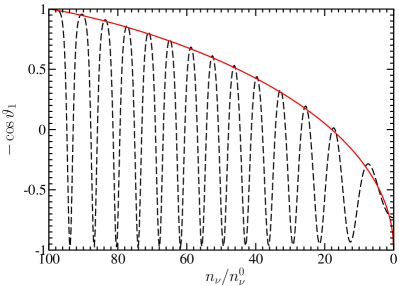
Figure 2: (Color online) Flavor oscillations of the simple symmetric bipolar system in a nearly adiabatic process [Eq. (34) with $\gamma=10$ and $n_{\nu}(0)/n_{\nu}^{0}=100$] for $\tilde{\theta}_{\mathrm{v}}=0.01$. The dashed line is the value of $-\cos\vartheta_{1}$ as a function $n_{\nu}$ computed from Eq. (3) with the initial conditions in Eq. (4). The solid line is $-\cos\vartheta_{\max}$ computed from Eq. (30).

An interesting scenario is that $\tilde{\theta}_{\mathrm{v}}=\pi/2-\theta_{\mathrm{v}}\ll 1$. In this case, $\bm{\hat{\mathbf{e}}}^{\mathrm{f}}_{z}\simeq-\mathbf{H}_{\mathrm{V}}$ and the probability for a neutrino to be $\nu_{e}$ is

$$P_{\nu_{e}\nu_{e}}=\frac{1}{2}+\mathbf{s}_{1}\cdot\bm{\hat{\mathbf{e}}}^{\mathrm{f}}_{z}\simeq\frac{1-\cos\vartheta_{1}}{2}\lesssim\frac{1-\cos\vartheta_{\max}}{2},$$ (31)

where $\vartheta_{1}$ is the angle between the directions of $\mathbf{s}_{1}$ and $\mathbf{H}_{\mathrm{V}}$. Noting that $W(2\theta_{\mathrm{v}})\simeq W(\pi)=1$, we find that

$$0\lesssim P_{\nu_{e}\nu_{e}}(t)\leq(P_{\nu_{e}\nu_{e}})_{\max},$$ (32)

where

$$(P_{\nu_{e}\nu_{e}})_{\max}\simeq\frac{1}{2}\left[1-\cos\left(W^{-1}\left(\sqrt{\frac{n_{\nu}(t)}{n_{\nu}(0)}}\right)\right)\right]$$ (33)

is the maximal value that $P_{\nu_{e}\nu_{e}}$ may take for a given $n_{\nu}$. In the above equation $W^{-1}(\xi)$ is the corresponding inverse function of $W(\xi)$.

For a concrete example, we assume that $n_{\nu}(t)$ has a linear dependence on time $t$:

$$n_{\nu}(t)=n_{\nu}(0)(1-\gamma^{-1}\mu_{\mathrm{V}}t),$$ (34)

where $\gamma$ is the adiabatic parameter. The larger the value of $\gamma$, the more adiabatic the process is. Taking $\tilde{\theta}_{\mathrm{v}}=0.01$, we calculate the value of $-\cos\vartheta_{1}$ as a function of $n_{\nu}$ for $\gamma=10$ and $n_{\nu}(0)/\nu_{\nu}^{0}=100$ by solving Eq. (3) with the initial conditions in Eq. (4). The results are plotted as the dashed line in Fig. 2. We have also computed $\vartheta_{\max}$ from Eq. (30) and plot $-\cos\vartheta_{\max}$ as the solid line in Fig. 2. It is clear that $-\cos\vartheta_{\max}$ outlines the upper envelope of $-\cos\vartheta_{1}$ for $n_{\nu}/n_{\nu}^{0}\gg 1$.

Using the analogy of harmonic oscillators, Ref. Hannestad et al. (2006) has argued that, for the scenario with $\tilde{\theta}_{\mathrm{v}}\ll 1$, $(P_{\nu_{e}\nu_{e}})_{\max}$ should depend linearly on $\sqrt{n_{\nu}}$, at least when $\vartheta_{\max}\ll 1$. However, it is clear that this conjecture is not true if $\vartheta_{\max}$ is significant. In this case, $(P_{\nu_{e}\nu_{e}})_{\max}$ can be understood using the general form of $W(\xi)$ and Eq. (33). On the other hand, we note that

$$W(\vartheta_{\max})\simeq\frac{\pi}{4}\left(\frac{\vartheta_{\max}}{2}\right)^{2}$$ (35)

for $\vartheta_{\max}\ll 1$ Gradshteyn and Ryzhik (1994). Using Eqs. (30) and (35) we obtain

$$\frac{\vartheta_{\max}^{2}(t)}{\vartheta_{\max}^{2}(t_{0})}\simeq\sqrt{\frac{n_{\nu}(t)}{n_{\nu}(t_{0})}},$$ (36)

where $t_{0}$ is an instant at which $\vartheta_{\max}(t_{0})\ll 1$. Because $P_{\nu_{e}\nu_{e}}\simeq(1-\cos\vartheta_{1})/2\simeq\vartheta_{1}^{2}/4$, we have

$$(P_{\nu_{e}\nu_{e}})_{\mathrm{\max}}\simeq\frac{\vartheta_{\max}^{2}(t_{0})}{4}\sqrt{\frac{n_{\nu}}{n_{\nu}(t_{0})}}$$ (37)

for $P_{\nu_{e}\nu_{e}}\ll 1$. Therefore, $(P_{\nu_{e}\nu_{e}})_{\max}$ does depend linearly on $\sqrt{n_{\nu}}$ in the limit $\vartheta_{\max}\ll 1$. Note that this result only applies for $n_{\nu}/n_{\nu}^{0}\gg 1$. As mentioned above, our argument about the adiabatic invariant fails for $n_{\nu}/n_{\nu}^{0}\lesssim 1$.

III Asymmetric Bipolar System

III.1 Gyroscopic flavor pendulum

We now consider a simple asymmetric bipolar system initially consisting of mono-energetic $\nu_{e}$ and $\bar{\nu}_{e}$ with different but constant number densities. We note that Eq. (3) is still valid except that we now take $n_{\nu,1}=n_{\nu}$ and $n_{\nu,2}=\alpha n_{\nu}$ with $\alpha\neq 1$ being a positive constant. Ref. Hannestad et al. (2006) has shown that this asymmetric bipolar system is equivalent to a gyroscopic pendulum or a spinning top in flavor space for which

$$\mathbf{S}_{+}(0) =\frac{1-\alpha}{2}n_{\nu}\bm{\hat{\mathbf{e}}}^{\mathrm{f}}_{z}$$ (38a)

$$\mathbf{S}_{-}(0) =\frac{1+\alpha}{2}n_{\nu}\bm{\hat{\mathbf{e}}}^{\mathrm{f}}_{z}.$$ (38b)

To see this we define

$$\mathbf{Q}\equiv\mathbf{S}_{-}-\frac{\mu_{\mathrm{V}}}{\mu_{\nu}}\mathbf{H}_{\mathrm{V}}.$$ (39)

(Although we follow Ref. Hannestad et al. (2006) in demonstrating the equivalence of an asymmetric bipolar system and a gyroscopic pendulum, we have adopted somewhat different notations for our convenience.) Using Eqs. (11b) and (39) one sees that $\mathbf{Q}$ obeys the e.o.m.

$$\frac{\mathrm{d}}{\mathrm{d}t}\mathbf{Q}=\mu_{\nu}{\mathbf{Q}}\times\mathbf{S}_{+}$$ (40)

and maintains a constant magnitude

$$\begin{split}Q=n_{\nu}\left(\frac{1+\alpha}{2}\right)\Bigg{[}&1+\left(\frac{4}{1+\alpha}\right)\left(\frac{n_{\nu}^{0}}{n_{\nu}}\right)\cos 2\theta_{\mathrm{v}}\\ &+\left(\frac{2}{1+\alpha}\right)^{2}\left(\frac{n_{\nu}^{0}}{n_{\nu}}\right)^{2}\Bigg{]}^{1/2}.\end{split}$$ (41)

With the definition of

$$\mathbf{J} \equiv\frac{\mathbf{S}_{+}}{n_{\nu}},$$ (42a)

$$\mathbf{r} \equiv\frac{\mathbf{Q}}{Q},$$ (42b)

Eqs. (11a), (39) and (40) lead to

$$\dot{\mathbf{J}} =\frac{\mu_{\mathrm{V}}Q}{n_{\nu}}\mathbf{r}\times\mathbf{H}_{\mathrm{V}},$$ (43a)

$$\dot{\mathbf{r}} =-\mu_{\mathrm{V}}\left(\frac{n_{\nu}}{n_{\nu}^{0}}\right)\mathbf{r}\times\mathbf{J}.$$ (43b)

Using Eq. (43) one can easily show that

$$\sigma\equiv\mathbf{J}\cdot\mathbf{r}$$ (44)

is a constant of motion. From Eq. (43b) one obtains

$$\mathbf{r}\times\dot{\mathbf{r}}=-\mu_{\mathrm{V}}\left(\frac{n_{\nu}}{n_{\nu}^{0}}\right)(\sigma\mathbf{r}-\mathbf{J}).$$ (45)

We note that Eqs. (43a) and (45) are equivalent to

$$\dot{\mathbf{J}} =\mathbf{r}\times M\mathbf{g},$$ (46a)

$$\mathbf{J} =M\mathbf{r}\times\dot{\mathbf{r}}+\sigma\mathbf{r},$$ (46b)

where

$$M =\frac{1}{\mu_{\mathrm{V}}}\left(\frac{n_{\nu}^{0}}{n_{\nu}}\right),$$ (47)

$$\mathbf{g} =\frac{\mu_{\mathrm{V}}^{2}}{n_{\nu}^{0}}Q\mathbf{H}_{\mathrm{V}}.$$ (48)

Therefore, this asymmetric bipolar system is indeed equivalent to a gyroscopic flavor pendulum. Specifically, $\mathbf{r}$ is the position vector of the bob, $\mathbf{J}$ is the total angular momentum, $\sigma$ is the internal angular momentum of the bob, $M$ is the mass of the bob, and $\mathbf{g}$ is the acceleration field. The only difference between this pendulum and that shown in Fig. 1(a) is the spin of the bob. Hereafter we will loosely refer to both the symmetric and asymmetric bipolar systems as flavor pendulums.

The motion of the gyroscopic flavor pendulum is the combination of a precession around $\mathbf{H}_{\mathrm{V}}$ and a nutation with $\vartheta_{\min}\leq\vartheta\leq\vartheta_{\max}$. Here $\vartheta$ is the polar angle of $\mathbf{r}$ with respect to $\bm{\hat{\mathbf{e}}}^{\mathrm{v}}_{z}=\mathbf{H}_{\mathrm{V}}$, and $\vartheta_{\min}$ and $\vartheta_{\max}$ are the minimal and maximal values of $\vartheta$ during nutation. For the simple asymmetric bipolar system that we have discussed, one has $\vartheta_{\max}=\vartheta|_{t=0}$. The value of $\vartheta_{\min}$ can be determined as follows. Following Ref. Hannestad et al. (2006) we define the total energy of the pendulum as

$$E_{\mathrm{tot}} =E_{\mathrm{pot}}+E_{\mathrm{kin}}$$ (49a)

$$=Mg(1-\mathbf{H}_{\mathrm{V}}\cdot\mathbf{r})+\frac{\mathbf{J}^{2}}{2M}$$ (49b)

$$=Mg(1-\cos\vartheta)+\frac{M\dot{\mathbf{r}}^{2}}{2}+\frac{\sigma^{2}}{2M}.$$ (49c)

We note that $E_{\mathrm{tot}}$ differs from the conserved total effective energy of the NFIS’s Duan et al. (2005) by only a constant multiplicative factor and a additive constant, and therefore, is also conserved. Because the motion of the pendulum is a pure precession around $\mathbf{H}_{\mathrm{V}}$ when $\vartheta=\vartheta_{\min}$, one has

$$Mg(\cos\vartheta_{\min}-\cos\vartheta_{\max})=\frac{1}{2}M\sin^{2}\vartheta_{\min}\dot{\varphi}^{2}|_{\vartheta=\vartheta_{\min}},$$ (50)

where $\varphi$ is the azimuthal angle of $\mathbf{r}$ with respect to $\mathbf{H}_{\mathrm{V}}$. Using the conservation of the total angular momentum in the direction of the acceleration field $\mathbf{g}$, one obtains

$$\sigma(\cos\vartheta_{\min}-\cos\vartheta_{\max})=-M\sin^{2}\vartheta_{\min}\,\dot{\varphi}|_{\vartheta=\vartheta_{\min}}.$$ (51)

Combining Eqs. (50) and (51) we have

$$\cos\vartheta_{\min}=-\eta+\sqrt{(\eta+\cos\vartheta_{\max})^{2}+(1-\cos^{2}\vartheta_{\max})},$$ (52)

where

$$\eta\equiv\frac{\sigma^{2}}{4M^{2}g}.$$ (53)

III.2 Precession/nutation modes and synchronized/bipolar regimes

We shall refer to neutrino flavor transformation as being in the precession (nutation) mode when the corresponding analogous flavor pendulum is undergoing precession (nutation). The symmetric bipolar system discussed in Sec. II corresponds to the limit $\alpha=1$ and is always in a pure nutation mode. In this limit $\sigma=0$ and $\vartheta_{\min}=0$, so the pendulum does not spin at all and simply swings in a fixed plane. Taking $p_{\vartheta}=\mathbf{J}\cdot\bm{\hat{\mathbf{e}}}^{\mathrm{v}}_{y}$ and $\vartheta$ as the angle between $\mathbf{r}$ and $\mathbf{H}_{\mathrm{V}}$, one can obtain from Eq. (43) that Hannestad et al. (2006)

$$\dot{p}_{\vartheta} =-\mu_{\mathrm{V}}\left(\frac{Q}{n_{\nu}}\right)\sin\vartheta$$ (54a)

$$\dot{\vartheta} =\mu_{\mathrm{V}}\left(\frac{n_{\nu}}{n_{\nu}^{0}}\right)p_{\vartheta}.$$ (54b)

Eq. (54) is the exact version of Eq. (16). In the limit $n_{\nu}/n_{\nu}^{0}\gg 1$, $\mathbf{Q}\simeq\mathbf{S}_{-}$ and $\mathbf{S}_{-}$ approximately follows a plane pendulum motion as we have discussed in Sec. II.1. If the neutrino number density $n_{\nu}$ is constant and the vacuum mixing angle $\theta_{\mathrm{v}}$ or $\tilde{\theta}_{\mathrm{v}}$ is small, the bipolar systems in the pure nutation mode can experience almost complete flavor conversion during a nutation period. This is true for various initial configurations (see Table I in Ref. Duan et al. (2005)).

A bipolar system generally evolves simultaneously in both precession and nutation modes. However, if the neutrino number density is large enough, it has been shown that a neutrino gas is in the synchronized mode with a characteristic frequency $\Omega_{\mathrm{sync}}$ independent of its initial configuration Pastor et al. (2002). The criterion for synchronization can be written as Duan et al. (2005)

$$|\mu_{\nu}\mathbf{S}|\gg|\langle\mu_{\mathrm{V}}\rangle|,$$ (55)

where

$$\mathbf{S}\equiv\sum_{i}n_{\nu,i}\mathbf{s}_{i}$$ (56)

is the total NFIS, and

$$\langle\mu_{\mathrm{V}}\rangle\equiv\sum_{i}\frac{\mu_{\mathrm{V},i}n_{\nu,i}\mathbf{s}_{i}\cdot\mathbf{S}}{\mathbf{S}^{2}}=\Omega_{\mathrm{sync}}$$ (57)

is the average vacuum oscillation frequency. The index $i$ in Eqs. (56) and (57) denotes neutrinos or antineutrinos with a specific momentum.

For the initial condition in Eq. (38) we note that, if $n_{\nu}$ is large, the total angular momentum of the flavor pendulum is dominated by its spin

$$\mathbf{J}\simeq\sigma\mathbf{r}$$ (58)

and

$$\sigma\simeq\frac{1-\alpha}{2}.$$ (59)

In the limit

$$n_{\nu}\gg n_{\nu}^{\mathrm{x}}\equiv 8\frac{1+\alpha}{(1-\alpha)^{2}}n_{\nu}^{0},$$ (60)

the parameter $\eta$ [see Eq. (53)] satisfies $\eta\gg 1$ and

$$\cos\vartheta_{\min}\simeq-\eta+\eta\left(1+\frac{\cos\vartheta_{\max}}{\eta}\right)\simeq\cos\vartheta_{\max}.$$ (61)

As a result, the flavor pendulum roughly maintains a constant latitude and is essentially in the precession mode. One can explicitly show that in this case the flavor pendulum precesses around $-\mathbf{H}_{\mathrm{V}}$ with a constant angular frequency Hannestad et al. (2006)

$$\Omega\simeq\Omega_{\mathrm{sync}}\equiv\frac{1+\alpha}{1-\alpha}\mu_{\mathrm{V}}.\quad$$ (62)

Therefore, a bipolar system is synchronized if $n_{\nu}\gg n_{\nu}^{\mathrm{x}}$ and the synchronized mode corresponds to a pure precession mode with the synchronization frequency $\Omega_{\mathrm{sync}}$ as its precession frequency. We refer to the limit in Eq. (60) as the “synchronized regime”. We say that a bipolar system is in the “bipolar regime” if Eq. (60) is not satisfied. In this case it can be in both the precession and nutation modes.

For the simple asymmetric bipolar system discussed here, Eq. (55) lead to

$$n_{\nu}\gg 2\frac{1+\alpha}{(1-\alpha)^{2}}n_{\nu}^{0}=\frac{n_{\nu}^{\mathrm{x}}}{4}.$$ (63)

Eqs. (60) and (63) differ by a constant multiplicative factor. This reflects the fact that there is no sharp boundary between the synchronized and bipolar regimes. The simple prescription for the synchronization frequency $\Omega_{\mathrm{sync}}$ in Eq. (57) allows a ready and practical application of the synchronization condition in Eq. (55) for neutrino and/or antineutrino gases with finite spreads in their energy spectra.

The ways in which the word “bipolar” has been used in the literature Duan et al. (2005, 2006a, 2006b); Hannestad et al. (2006); Raffelt and Sigl (2007) can be very confusing. There is a tendency to mistakenly identify the synchronized (bipolar) regime with the precession (nutation) mode. This is probably because a flavor pendulum can only precess in the synchronized regime and a symmetric bipolar system was once viewed as a typical bipolar system which is always in a nutation mode. However, the criterion determining whether a bipolar system is mostly in the precession or nutation mode is not the same as that for determining whether it is in the synchronized or bipolar regime. A good example is that an asymmetric bipolar system can simultaneously be in both the precession and nutation modes in the bipolar regime. We also note that, while the precession frequency $\Omega$ of the precession mode in the synchronized regime is determined from Eq. (57) and is independent of the neutrino number density $n_{\nu}$, the precession frequency of a precession mode in the bipolar regime depends on $n_{\nu}$ (see Sec. IV.3).

The evolution of a bipolar system in the bipolar regime is also referred to as bimodal oscillations. Ref. Samuel (1996) has shown that, in an asymmetric bipolar system initially consisting of mono-energetic $\nu_{e}$ and $\bar{\nu}_{e}$, the $x$- and $y$-components of the polarization vectors of the neutrino and antineutrino ($2\mathbf{s}_{1}$ and $-2\mathbf{s}_{2}$ in the NFIS notation) are bimodal as they are functions of two intrinsic periods. It is clear that these two periods are related to the precession and nutation of the flavor pendulum. If $\nu_{e}$ and $\bar{\nu}_{e}$ have different energies or the system starts with different neutrino/antineutrino species, one can demonstrate that such a system is equivalent to a flavor pendulum in some properly chosen corotating frame Duan et al. (2005). In this case the precession frequency $\Omega$ is shifted by the rotation frequency of the corotating frame.

IV Pure Precession Mode of Asymmetric Bipolar Systems

IV.1 Pure precession mode

$\begin{array}[]{@{}c@{\hspace{\myfigsep}}c@{}}\includegraphics*[width=208.13574pt,keepaspectratio]{fig3a.eps}\hfil\hskip 17.34189pt&\includegraphics*[width=208.13574pt,keepaspectratio]{fig3b.eps}\\ \includegraphics*[width=208.13574pt,keepaspectratio]{fig3c.eps}\hfil\hskip 17.34189pt&\includegraphics*[width=208.13574pt,keepaspectratio]{fig3d.eps}\end{array}$

Figure 3: (Color online) Values of $\cos\vartheta_{1}$ (solid lines) and $\cos\vartheta_{2}$ (dashed lines), where $\vartheta_{1}$ and $\vartheta_{2}$ are the polar angles of the NFIS’s $\mathbf{s}_{1}$ and $\mathbf{s}_{2}$ with respect to $\mathbf{H}_{\mathrm{V}}$, as functions of neutrino number density $n_{\nu}$ for simple asymmetric bipolar systems. Panels (a), (b) and (d) have mixing angle $\tilde{\theta}_{\mathrm{v}}=0.01$ and panel (c) has $\theta_{\mathrm{v}}=0.6$. The asymmetry parameter is $\alpha=0.8$ for (a) and (c), and $\alpha=0.2$ for (b) and (d). The thin lines are computed from the original e.o.m. of NFIS’s $\mathbf{s}_{1}$ and $\mathbf{s}_{2}$ [Eq. (3) with the initial conditions in (4)] assuming a nearly adiabatic process [Eq. (34) with $n_{\nu}(0)/n_{\nu}^{\mathrm{x}}=2$]. The adiabatic parameter is $\gamma=40$ for panels (a–c) and is $200$ for panel (d). The thick lines are computed from Eq. (66) assuming that bipolar systems stay in the pure precession mode. The vertical dot-dashed lines in panels (a), (b) and (d) correspond to $n_{\nu}=n_{\nu}^{\mathrm{c}}$.

Although a bipolar system tends to develop some nutation in addition to the precession mode in the bipolar regime, the actual mix of these modes depends on the initial conditions as well as the system configuration. For example, a flavor pendulum precesses around $-\mathbf{H}_{\mathrm{V}}$ with constant angular frequency $\Omega$ without any nutation if

$$Mg\sin\vartheta =\Omega J_{\perp}$$ (64a)

$$=\Omega(M\Omega\sin\vartheta\cos\vartheta+\sigma\sin\vartheta)$$ (64b)

is satisfied, and the corresponding bipolar system is in the pure precession mode. For a gyroscope this is known as the “regular precession”.

With varying neutrino number densities the problem is generally complicated. This is because almost all the parameters of the flavor pendulum ($Q$, $M$, $g$, $\sigma$, etc.) depend on $n_{\nu}$ and the e.o.m. of a pendulum, Eq. (46), is not equivalent to that of the NFIS’s if $n_{\nu}(t)$ is not constant. In this case, one has to use Eq. (3) to follow the evolution of the bipolar system. Simple numerical examples presented in Ref. Hannestad et al. (2006) seem to suggest that the evolution of a bipolar system with $\theta_{\mathrm{v}}\simeq\pi/2$ can be dominantly in a precession mode after the system transitions from the synchronized regime into the bipolar regime. Here we try to gain some analytical understanding of this precession mode by using the same simple bipolar system studied in Sec. III but with time-varying $n_{\nu}$.

We note that, in the synchronized regime (i.e., the limit of large $n_{\nu}$), both $\mathbf{s}_{1}$ and $\mathbf{s}_{2}$ precess uniformly around $\mathbf{H}_{\mathrm{V}}$, and the motion of the NFIS’s has a cylindrical symmetry around the axis along $\mathbf{H}_{\mathrm{V}}$. This symmetry is inherited from the e.o.m. of the NFIS’s [Eq. (3)]. We consider an infinitely long process during which $n_{\nu}$ is decreased without preference to any azimuthal angle with respect to $\mathbf{H}_{\mathrm{V}}$. The cylindrical symmetry in the motion of the NFIS’s around $\mathbf{H}_{\mathrm{V}}$ is expected to be preserved in such a process, and $\mathbf{s}_{1}$ and $\mathbf{s}_{2}$ keep on precessing uniformly around $\mathbf{H}_{\mathrm{V}}$ without any wobbling.

If this is true, vectors $\mathbf{s}_{1}$, $\mathbf{s}_{2}$ and $\mathbf{H}_{\mathrm{V}}$ must always be in the same plane, and $\mathbf{s}_{1}$ and $\mathbf{s}_{2}$ rotates around $-\mathbf{H}_{\mathrm{V}}$ with the same angular frequency

$$\Omega =\mu_{\mathrm{V}}\left[1-\frac{\alpha}{2\sin\vartheta_{1}}\left(\frac{n_{\nu}}{n_{\nu}^{0}}\right)\sin(\vartheta_{1}+\vartheta_{2})\right]$$ (65a)

$$=\mu_{\mathrm{V}}\left[-1-\frac{1}{2\sin\vartheta_{2}}\left(\frac{n_{\nu}}{n_{\nu}^{0}}\right)\sin(\vartheta_{1}+\vartheta_{2})\right],$$ (65b)

where $\vartheta_{1(2)}$ is the angle between $\mathbf{s}_{1(2)}$ and $\mathbf{H}_{\mathrm{V}}$. On the other hand, from Eq. (3) it can be shown that $\mathbf{H}_{\mathrm{V}}\cdot(\mathbf{s}_{1}+\alpha\mathbf{s}_{2})$ is time invariant even if $n_{\nu}$ changes with time. Consequently, we obtain the following two equations for $\vartheta_{1}$ and $\vartheta_{2}$:

$$4\sin\vartheta_{1}\sin\vartheta_{2} =-\frac{n_{\nu}}{n_{\nu}^{0}}(\sin\vartheta_{1}-\alpha\sin\vartheta_{2})$$

$$\quad\times\sin(\vartheta_{1}+\vartheta_{2}),$$ (66a)

$$(1-\alpha)\cos 2\theta_{\mathrm{v}} =\cos\vartheta_{1}+\alpha\cos\vartheta_{2}.$$ (66b)

We have solved Eq. (66) numerically for simple asymmetric bipolar systems with different choices of $\theta_{\mathrm{v}}$ and asymmetry parameter $\alpha$. The results are plotted in Fig. 3. For comparison, we have also solved numerically the original e.o.m. of the NFIS’s, Eq. (3), for the same bipolar systems assuming that $n_{\nu}$ changes in the way described by Eq. (34). These results are also shown in Fig. 3. Clearly, the polar angles $\vartheta_{1}$ and $\vartheta_{2}$ of the NFIS’s $\mathbf{s}_{1}$ and $\mathbf{s}_{2}$ oscillate around those values determined from Eq. (66) as $n_{\nu}$ decreases. This is true not only for the bipolar systems with $\theta_{\mathrm{v}}\simeq\pi/2$ but also for those with other vacuum mixing angles.

The results shown in Fig. 3 can be understood as follows. Although Eqs. (3) and (46) are not equivalent over a long period for a time-varying $n_{\nu}$, we may still view a bipolar system as a flavor pendulum over a short time interval during which $n_{\nu}$ does not change much. Suppose that at instant $t_{1}$ the flavor pendulum precesses uniformly around $\mathbf{H}_{\mathrm{V}}$ at latitude $\vartheta_{0}(t_{1})$. In the adiabatic limit this precession continues as $n_{\nu}$ slowly changes, but the value of $\vartheta_{0}$ changes with $n_{\nu}$ [$\vartheta_{0}$ is a function of $\vartheta_{1}$ and $\vartheta_{2}$ which vary with $n_{\nu}$ according to Eq. (66)]. Of course, in realistic conditions, $n_{\nu}$ can only decrease with a finite rate, and the actual polar angle $\vartheta$ of the pendulum always “wobbles” (as a result of excitation of nutation modes) around $\vartheta_{0}$ with some nutation period $T_{\mathrm{nut}}$. However, if $n_{\nu}$ changes so slowly that

$$\left[T_{\mathrm{nut}}\left(\frac{\mathrm{d}n_{\nu}}{\mathrm{d}t}\right)\right]^{-1}\gg\left(\frac{\mathrm{d}\vartheta_{0}}{\mathrm{d}n_{\nu}}\right),\,\left(\frac{\partial\vartheta}{\partial n_{\nu}}\right),$$ (67)

$\vartheta$ can be expected to closely follow $\vartheta_{0}$, and Eq. (66) becomes an excellent approximation. This expectation can be verified by comparing panels (b) and (d) of Fig. 3 where the evolution of two otherwise identical bipolar systems is calculated using different adiabatic parameters [$\gamma=40$ in (b) and $200$ in (d)]. With a much slower change in $n_{\nu}$ for panel (d), the result obtained by solving Eq. (66) becomes very close to that derived from the exact numerical calculations.

The final values of $\vartheta_{1}|_{n_{\nu}=0}$ and $\vartheta_{2}|_{n_{\nu}=0}$ of the bipolar system in the pure precession mode can be obtained as follows. The precession frequency $\Omega$ of the flavor pendulum cannot be 0, and therefore, cannot change sign as $n_{\nu}$ decreases. Because $\Omega=\Omega_{\mathrm{sync}}>0$ in the limit of large $n_{\nu}$ for $\alpha<1$ [Eq. (62)], we have $\Omega>0$. Eq. (65b) would give $\Omega>0$ for $n_{\nu}=0$ only if

$$\vartheta_{2}|_{n_{\nu}=0}=\pi.$$ (68)

This and Eq. (65) then give

$$\Omega|_{n_{\nu}=0}=\mu_{\mathrm{V}}.$$ (69)

Combining Eqs. (68) and (66b) we obtain

$$\cos\vartheta_{1}|_{n_{\nu}=0}=(1-\alpha)\cos 2\theta_{\mathrm{v}}+\alpha.$$ (70)

This agrees with the numerical results shown in Fig. 3. For the inverted mass hierarchy scenario with $\theta_{\mathrm{v}}\simeq\pi/2$, we have $\bm{\hat{\mathbf{e}}}^{\mathrm{f}}_{z}\simeq-\mathbf{H}_{\mathrm{V}}$ and

$$P_{\nu_{e}\nu_{e}}|_{n_{\nu}=0} \simeq\left.\frac{1-\cos\vartheta_{1}}{2}\right|_{n_{\nu}=0}\simeq 1-\alpha,$$ (71a)

$$P_{\bar{\nu}_{e}\bar{\nu}_{e}}|_{n_{\nu}=0} \simeq\left.\frac{1+\cos\vartheta_{2}}{2}\right|_{n_{\nu}=0}\simeq 0.$$ (71b)

However, we note that these results for $n_{\nu}=0$ do not apply to realistic bipolar systems with finite spreads in the neutrino and antineutrino energy spectra as collective oscillations of these systems always break down before $n_{\nu}$ reaches 0.

IV.2 Critical neutrino number density for the inverted mass hierarchy scenario with $\theta_{\mathrm{v}}\simeq\pi/2$

In Fig. 3 one can see that, for the inverted mass hierarchy scenario with $\theta_{\mathrm{v}}\simeq\pi/2$, $\mathbf{s}_{1}$ and $\mathbf{s}_{2}$ begin to misalign with $\mathbf{H}_{\mathrm{V}}$ when $n_{\nu}$ is smaller than some critical value $n_{\nu}^{\mathrm{c}}$, and there seems to be discontinuity in $\mathrm{d}\vartheta_{1(2)}/\mathrm{d}n_{\nu}$ at $n_{\nu}=n_{\nu}^{\mathrm{c}}$. To understand these results, we consider the limit where $\theta_{\mathrm{v}}=\pi/2$. We define

$$x_{1(2)}\equiv\sin\vartheta_{1(2)}.$$ (72)

For $\vartheta_{1}\simeq\pi$ and $\vartheta_{2}\simeq 0$ we have

$$\cos\vartheta_{1} \simeq-1+\frac{x_{1}^{2}}{2},$$ (73a)

$$\cos\vartheta_{2} \simeq 1-\frac{x_{2}^{2}}{2}.$$ (73b)

Combining Eqs. (66) and (73) we obtain

$$4x_{1}x_{2} \simeq(x_{1}-\alpha x_{2})\frac{n_{\nu}}{n_{\nu}^{0}}$$

$$\quad\times\left[x_{2}\left(1-\frac{x_{1}^{2}}{2}\right)-x_{1}\left(1-\frac{x_{2}^{2}}{2}\right)\right],$$ (74a)

$$1-\alpha \simeq\left(1-\frac{x_{1}^{2}}{2}\right)-\alpha\left(1-\frac{x_{2}^{2}}{2}\right).$$ (74b)

Eq. (74) has the solution

$$x_{1}^{2}\simeq\alpha x_{2}^{2}\simeq 2\sqrt{\alpha}\left(\frac{n_{\nu}^{\mathrm{c}}}{n_{\nu}}-1\right)\quad\mathrm{if}\,n_{\nu}<n_{\nu}^{\mathrm{c}},$$ (75)

where

$$n_{\nu}^{\mathrm{c}}\equiv\frac{4n_{\nu}^{0}}{(1-\sqrt{\alpha})^{2}}.$$ (76)

Therefore, for the limiting case with $\theta_{\mathrm{v}}=\pi/2$, $\mathbf{s}_{1}$ and $\mathbf{s}_{2}$ only start to misalign with $\mathbf{H}_{\mathrm{V}}$ when $n_{\nu}$ becomes smaller than $n_{\nu}^{\mathrm{c}}$.

One can also obtain the same value for $n_{\nu}^{\mathrm{c}}$ from the gyroscopic flavor pendulum analogy using Eq. (52). For $\vartheta_{\max}=\pi$, one always has $\vartheta_{\min}=\pi$ if

$$\eta=\frac{\sigma^{2}}{4M^{2}g}>1.$$ (77)

Such a gyroscopic pendulum is known as a “sleeping top” because the pendulum “sleeps” in the upright position defying the effect of the gravity (see, e.g., Ref. Scarborough (1958) for more discussions).

We note that the period of nutation $T_{\mathrm{nut}}$ of the flavor pendulum is infinite if $\theta_{\mathrm{v}}=\pi/2$. For a symmetric bipolar system $T_{\mathrm{nut}}\propto|\ln\tilde{\theta}_{\mathrm{v}}|$ if $\theta_{\mathrm{v}}\simeq\pi/2$ (see Sec. II.1 and also Ref. Hannestad et al. (2006)). One expects similarly long nutation periods for asymmetric bipolar systems in the region where $n_{\nu}\simeq n_{\nu}^{\mathrm{c}}$. In the same region, $\vartheta_{1}$ and $\vartheta_{2}$ change very quickly in the pure precession limit. As a result, the condition in Eq. (67) is usually violated in realistic environments and significant nutation can appear for $n_{\nu}<n_{\nu}^{\mathrm{c}}$ [see, e.g., Fig. 3(b)].

IV.3 Precession frequency

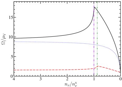
Figure 4: (Color online) Scaled precession frequency $\Omega/\mu_{\mathrm{V}}$ of the flavor pendulum as a function of neutrino number density $n_{\nu}$. The pendulum is assumed to be in the pure precession mode. The vacuum mixing angle is $\tilde{\theta}_{\mathrm{v}}=0.01$ for the solid and dashed lines, and $\theta_{\mathrm{v}}=0.6$ for the dotted line. The asymmetry parameter is $\alpha=0.8$ for the solid and dotted lines and is $0.2$ for the dashed line. The vertical dot-dashed line and dot-dot-dashed line correspond to $n_{\nu}=n_{\nu}^{\mathrm{c}}$ for $\alpha=0.8$ and $0.2$, respectively.

Using Eq. (65) we have calculated the precession frequency $\Omega$ of the flavor pendulum for several scenarios assuming the pendulum is always in the pure precession mode. The results are plotted in Fig. 4. The precession frequency $\Omega$ asymptotically approaches the synchronization frequency $\Omega_{\mathrm{sync}}$ in the synchronized regime ($n_{\nu}/n_{\nu}^{\mathrm{x}}\gg 1$) as $n_{\nu}$ becomes larger and larger. On the other hand, $\Omega$ changes steeply with $n_{\nu}$ in the bipolar regime ($n_{\nu}/n_{\nu}^{\mathrm{x}}\lesssim 1$). As $n_{\nu}$ reaches 0, $\Omega=\mu_{\mathrm{V}}$ and the flavor pendulum precesses with the vacuum oscillation frequency of the dominant neutrino species ($\nu_{e}$ in this case).

We also note that, for the inverted mass hierarchy scenario with $\theta_{\mathrm{v}}\simeq\pi/2$, the precession frequency $\Omega$ reaches its maximum at $n_{\nu}\simeq n_{\nu}^{\mathrm{c}}$. Using Eqs. (65) and (75), we obtain

$$\Omega|_{n_{\nu}=n_{\nu}^{\mathrm{c}}}=1+\frac{2\sqrt{\alpha}}{1-\sqrt{\alpha}}\quad\text{for}\,\theta_{\mathrm{v}}=\frac{\pi}{2},$$ (78)

which is $17.9$ for $\alpha=0.8$ and $2.6$ for $\alpha=0.2$. These values agree well with the solid and dashed lines in Fig. 4 which assume $\tilde{\theta}_{\mathrm{v}}=0.01$.

IV.4 Equipartition of energies?

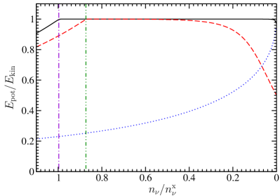
Figure 5: (Color online) Ratio of the potential energy $E_{\mathrm{pot}}$ of the flavor pendulum to its kinetic energy $E_{\mathrm{kin}}$ [Eq. (49)] as functions of neutrino number density $n_{\nu}$. The parameters and the meaning of the lines are the same as those in Fig. 4.

Ref. Hannestad et al. (2006) observed that, for $\theta_{\mathrm{v}}\simeq\pi/2$, the total energy of a flavor pendulum begins to be approximately equipartitioned between its potential and kinetic energies when $n_{\nu}$ reaches $n_{\nu}^{\mathrm{c}}$. Using Eq. (75) one can show that (see Appendix A), for the extreme case $\theta_{\mathrm{v}}=\pi/2$, the ratio of energies is $E_{\mathrm{pot}}/E_{\mathrm{kin}}\simeq 1$ to $\mathcal{O}(n_{\nu}^{\mathrm{c}}/n_{\nu}-1)$ at $n_{\nu}\simeq n_{\nu}^{\mathrm{c}}$ if the flavor pendulum stays in the pure precession mode.

Ref. Hannestad et al. (2006) also mentioned “an important detail” that energy equipartition cannot hold all the way down to very small $n_{\nu}$ because $E_{\mathrm{pot}}$ has a finite positive minimum and $E_{\mathrm{kin}}$ ultimately reaches 0. This is illustrated in Fig. 8 of the same reference. However, we can show that (see Appendix A)

$$\frac{E_{\rm pot}}{E_{\rm kin}}\simeq 1-\frac{(1-\alpha)\cos^{2}2\theta_{\mathrm{v}}}{1+\alpha-2\alpha\cos 2\theta_{\mathrm{v}}}\quad\text{for}\,\left(\frac{n_{\nu}}{n_{\nu}^{0}}\right)\ll 1$$ (79)

if the flavor pendulum stays in the pure precession mode.

In Fig. 5 we plot the ratio $E_{\mathrm{pot}}/E_{\mathrm{kin}}$ as a function $n_{\nu}$ for three different bipolar systems in the pure precession mode with various choices of $\alpha$ and $\theta_{\mathrm{v}}$. Indeed, for the bipolar systems with $\theta_{\mathrm{v}}\simeq\pi/2$, $E_{\mathrm{pot}}/E_{\mathrm{kin}}$ reaches 1 at $n_{\nu}=n_{\nu}^{\mathrm{c}}$ and does not change much for a significant range of $n_{\nu}$. This is especially true for $\alpha\simeq 1$. In the limit $n_{\nu}=0$, $E_{\rm pot}/E_{\rm kin}\simeq 0.94$ and 0.5 for $\theta_{\mathrm{v}}\simeq\pi/2$ but $\alpha=0.8$ and 0.2, respectively. In the same limit, $E_{\rm pot}/E_{\rm kin}\simeq 0.98$ for $\theta_{\mathrm{v}}=0.6$ and $\alpha=0.8$. These results agree well with Eq. (79).

V Neutrino Oscillations in Supernovae

Refs. Duan et al. (2006a, b) have presented two sets of simulations using the “single-angle” and “multi-angle” approximations, respectively. These simulations together with the simple analytical and numerical models discussed in the previous sections represent approximations to the real supernova neutrino oscillation problem at three different levels of complexity.

The analytical and numerical calculations performed in this paper assume that the neutrino gas is homogeneous and isotropic and is represented by two mono-energetic neutrino and/or antineutrino species.

The single-angle simulations increase the complexity by allowing each neutrino species (4 in the $2\times 2$ case) to have continuous energy distributions. It assumes that the flavor evolution histories of neutrinos propagating along different trajectories are the same as those of neutrinos emitted radially from the neutrino sphere. Although the single-angle approximation incorporates the angle dependence of neutrino-neutrino forward scattering into the “effective neutrino density” Duan et al. (2006a), it still assumes that neutrino on all trajectories evolve similarly.

The multi-angle simulations are by far the most sophisticated treatment of the problem. In these calculations neutrinos and antineutrinos have not only continuous energy distributions but also continuous angular distributions. The most important improvement implemented in the multi-angle simulations is that the flavor evolution of neutrinos and antineutrinos (with a wide range of energies) propagating along different trajectories is followed independently.

In this section we will first apply our simple models to the single-angle calculations. We will discuss the onset of neutrino flavor conversion in both the inverted and normal mass hierarchy scenarios (Secs. V.1 and V.2). We will also investigate the precession mode of the neutrino gas in supernovae and its effects (Sec. V.3). Finally, we will offer some new analyses of the multi-angle simulations and comment on the collectivity of neutrino flavor transformation in supernovae (Sec. V.4).

V.1 Onset of neutrino flavor conversion in the inverted mass hierarchy scenario

The simulations presented in Refs. Duan et al. (2006a, b) for the inverted neutrino mass hierarchy scenario all have $\tilde{\theta}_{\mathrm{v}}=0.1$. According to the discussions in Sec. IV.2, bipolar neutrino systems with vacuum mixing angle $\theta_{\mathrm{v}}\simeq\pi/2$ can start flavor conversion after the neutrino number density $n_{\nu}$ drops below some critical value $n_{\nu}^{\mathrm{c}}$. Although the conclusion was made in the absence of an ordinary matter background, it has been shown that the evolution of bipolar systems is not changed qualitatively even in a dominant matter background as long as $\theta_{\mathrm{v}}\simeq\pi/2$ Duan et al. (2005); Hannestad et al. (2006).

For a rough estimate of the radius where $n_{\nu}=n_{\nu}^{\mathrm{c}}$, we assume that the neutrino gas behaves in a way similar to the simple bipolar system initially consisting of $\nu_{e}$ and $\bar{\nu}_{e}$ with energies $E_{\nu_{e}}=11\,\mathrm{MeV}$ and $E_{\bar{\nu}_{e}}=16\,\mathrm{MeV}$, respectively. (These values are the same as the average energies of $\nu_{e}$ and $\bar{\nu}_{e}$ in the simulations.) In a properly chosen corotating frame, the evolution of this simplified bipolar system is the same as that of a gas initial consisting of mono-energetic $\nu_{e}$ and $\bar{\nu}_{e}$ with energy Duan et al. (2005)

$$\overline{E}_{\nu} \equiv\left[\frac{1}{2}\left(\frac{1}{E_{\nu_{e}}}+\frac{1}{E_{\bar{\nu}_{e}}}\right)\right]^{-1}$$ (80a)

$$\simeq 13\,\mathrm{MeV}.$$ (80b)

With the luminosities of all neutrino species being the same and $L_{\nu}=10^{51}\,\mathrm{erg/s}$, the ratio of the number densities of the two neutrino species is

$$\alpha=\frac{L_{\nu}/E_{\bar{\nu}_{e}}}{L_{\nu}/E_{\nu_{e}}}\simeq 0.69.$$ (81)

Therefore, the critical neutrino number density is [see Eq. (76)]

$$n_{\nu}^{\mathrm{c}} =\frac{\delta m^{2}}{\sqrt{2}G_{\mathrm{F}}\overline{E}_{\nu}}(1-\sqrt{\alpha})^{-2}$$ (82a)

$$\simeq 6.24\times 10^{28}\,\mathrm{cm}^{-3}$$ (82b)

for a mass squared difference $\delta m^{2}=3\times 10^{-3}\,\mathrm{eV}^{2}$. Using the single-angle approximation we estimate the effective neutrino number density to be

$$n_{\nu}^{\mathrm{eff}}(r) =\frac{L_{\nu}}{4\pi R_{\nu}^{2}E_{\nu_{e}}}\left[1-\sqrt{1-\left(\frac{R_{\nu}}{r}\right)^{2}}\right]^{2}$$ (83a)

$$\simeq(1.25\times 10^{32}\,\mathrm{cm}^{-3})\left[1-\sqrt{1-\left(\frac{R_{\nu}}{r}\right)^{2}}\right]^{2},$$ (83b)

where $R_{\nu}=11\,\mathrm{km}$ is the radius of the neutrino sphere adopted in the simulation. Therefore, $n_{\nu}^{\mathrm{eff}}\simeq n_{\nu}^{\mathrm{c}}$ at radius $r_{\mathrm{c}}\simeq 52\,\mathrm{km}$.

From panels (c) and (d) of Fig. 8 in Ref. Duan et al. (2006a) one sees that, in the single angle simulation, the flavor conversion starts at the radius $r_{\mathrm{X}}\simeq 63\,\mathrm{km}$. At $r\gtrsim r_{\mathrm{X}}$ the $z$-components of NFIS’s $\mathbf{s}_{\nu_{e}}$ experience rapid oscillations which correspond to the nutation mode of the flavor pendulum. The estimated value of $r_{\mathrm{c}}\simeq 52\,\mathrm{km}$ and the observed value of $r_{\mathrm{X}}\simeq 63\,\mathrm{km}$ differ by $\sim 10\,\mathrm{km}$. This difference most likely arises because at $r\simeq r_{\mathrm{c}}$ the nutation frequency $T_{\mathrm{nut}}^{-1}$ of the flavor pendulum is very small. Consequently, there is a delay before significant nutation amplitude can develop. On the other hand, smaller nutation frequency implies less adiabatic evolution [see Eq. (67)]. So once developed, the nutation amplitude will be large. The oscillation amplitudes of $\langle s_{\nu_{e}z}\rangle$ and $\langle s_{\bar{\nu}_{e}z}\rangle$ are indeed large as shown in Fig. 8 of Ref. Duan et al. (2006a).

We note that the region ($r_{\mathrm{c}}\lesssim r\lesssim r_{\mathrm{X}}$) where the nutation modes are to be excited is roughly the same region where the chaos-like phenomenon shown in Fig. 12 of Ref. Duan et al. (2006a) occurs. In this region the differences of two almost identical systems can grow exponentially as they evolve.

V.2 Onset of neutrino flavor conversion in the normal mass hierarchy scenario

The simulations presented in Refs. Duan et al. (2006a, b) for the normal neutrino mass hierarchy scenario all have $\theta_{\mathrm{v}}=0.1$. According to the discussions in Sec. III, a bipolar neutrino system with vacuum mixing angle $\theta_{\mathrm{v}}\ll 1$ corresponds to a flavor pendulum that oscillates in a very limited region near the bottom of the potential well, and therefore, does not experience much flavor transformation. However, this conclusion only applies in the absence of an ordinary matter background.

In the presence of a matter background, it has been shown that, in the synchronized regime, neutrinos and antineutrinos of all the species and energies go through an MSW-like resonance simultaneously in the same way as does a neutrino with the characteristic energy $E_{\mathrm{sync}}$ in the conventional MSW picture Pastor and Raffelt (2002). A similar phenomenon may also occur in bipolar systems in the bipolar regime (i.e., outside the synchronized regime) as suggested in Ref. Duan et al. (2005). If this is true, the dominant neutrino species are changed from $\nu_{e}$ and $\bar{\nu}_{e}$ to $\nu_{\mu,\tau}$ and $\bar{\nu}_{\mu,\tau}$. Using the corotating frame, one can show that the evolution of a $\bar{\nu}_{\mu,\tau}$-$\nu_{\mu,\tau}$ gas with the normal mass hierarchy is similar to that of a $\nu_{e}$-$\bar{\nu}_{e}$ gas with the inverted mass hierarchy Duan et al. (2005), and the flavor pendulum is raised from the bottom position to the top position because of the change in the dominant neutrino species. Bipolar systems can subsequently develop nutation modes after the collective MSW-like resonance.

From panels (a) and (b) of Fig. 8 in Ref. Duan et al. (2006a) one sees that, in the single angle simulation, the $z$-components of NFIS’s $\mathbf{s}_{\nu_{e}}$ suddenly change at radius $r_{\mathrm{X}}\simeq 88\,\mathrm{km}$ and oscillate rapidly afterwards. This corresponds to the initial collective MSW-like resonance followed by the nutation modes. We note that the observed value of $r_{\mathrm{X}}$ in the simulation is larger than the value of $74\,\mathrm{km}$ estimated for the fully synchronized limit Duan et al. (2006a). The difference arises partly because the MSW-like resonance actually occurs in the bipolar regime in this case.

V.3 Precession mode and final neutrino survival probabilities

As shown in Sec. III bipolar systems generally are in both precession and nutation modes. This is indeed seen in the single-angle simulations for both the normal and inverted mass hierarchies. In Fig. 8 of Ref. Duan et al. (2006a), the $x$- and $y$-components of NFIS’s $\mathbf{s}_{\nu_{e}}$ oscillate with an approximate phase difference of $\pi/2$, signifying precession in the $x$-$y$ plane.

In Sec. IV.1 we have argued that, in the absence of an ordinary matter background, the intrinsic precession angular velocity $\bm{\Omega}$ of the bipolar system as a whole should be in the same direction as that of a single neutrino of the dominant species. Therefore, we expect bipolar systems dominated by neutrinos to tend to precess around $-\mathbf{H}_{\mathrm{V}}$. In the presence of a matter background, bipolar systems will also tend to precess around the direction opposite to

$$\mathbf{H}_{e}\equiv-\bm{\hat{\mathbf{e}}}^{\mathrm{f}}_{z}\sqrt{2}G_{\mathrm{F}}n_{e},$$ (84)

where $n_{e}$ is the net electron number density. For the inverted mass hierarchy with $\theta_{\mathrm{v}}\simeq\pi/2$ and $\mathbf{H}_{\mathrm{V}}\simeq-\bm{\hat{\mathbf{e}}}^{\mathrm{f}}_{z}$, the intrinsic $\bm{\Omega}$ of the flavor pendulum is roughly in the same direction as the precession stemming from the matter background. In this case, the combined precession does not change direction. As a result, the precession of NFIS’s is always roughly around $-\mathbf{H}_{\mathrm{V}}\simeq\bm{\hat{\mathbf{e}}}^{\mathrm{f}}_{z}$ for the inverted mass hierarchy.

For the normal mass hierarchy with $\theta_{\mathrm{v}}\ll 1$ and $\mathbf{H}_{\mathrm{V}}\simeq\bm{\hat{\mathbf{e}}}^{\mathrm{f}}_{z}$, the intrinsic $\bm{\Omega}$ of the flavor pendulum is roughly in the opposite direction to that of the precession due to the matter background, and the combined precession may change its direction. However, it is expected that the matter background becomes negligible after the collective MSW-like resonance. Therefore, the NFIS’s precess roughly in the direction of $-\mathbf{H}_{\mathrm{V}}\simeq-\bm{\hat{\mathbf{e}}}^{\mathrm{f}}_{z}$ in the region $r\gtrsim r_{\mathrm{X}}$ for the normal mass hierarchy. According to Fig. 8 of Ref. Duan et al. (2006a) NFIS’s indeed precess around $\bm{\hat{\mathbf{e}}}^{\mathrm{f}}_{z}$ for the inverted mass hierarchy scenario and $-\bm{\hat{\mathbf{e}}}^{\mathrm{f}}_{z}$ for the normal mass hierarchy scenario.

Ref. Duan et al. (2006a) has shown that (see Fig. 9 of that reference), for the inverted mass hierarchy scenario and at large radius, neutrinos with energies below $E_{\mathrm{C}}\simeq 9\,\mathrm{MeV}$ are mostly in their initial flavors while neutrinos with larger energies and most antineutrinos can be completely converted to other flavors in the limit of large neutrino luminosity $L_{\nu}$. For the normal mass hierarchy scenario, neutrinos with energies below $E_{\mathrm{C}}\simeq 9\,\mathrm{MeV}$ are almost completely converted to other flavors while neutrinos with larger energies and nearly all antineutrinos are mostly in their initial flavors in the limit of large $L_{\nu}$. Ref. Duan et al. (2006a) suggested that this phenomenon is related to the precession of NFIS’s when neutrino number densities decrease and the bipolar configuration starts to break down (see Fig. 10 of that reference).

We note that the precession of NFIS’s due to the matter background $\mathbf{H}_{e}$ is the same for all neutrinos, and we can essentially ignore it in a reference frame $\mathcal{F}_{1}$ rotating with angular velocity $-\mathbf{H}_{e}$. In this corotating frame $\mathcal{F}_{1}$, the e.o.m. of NFIS $\mathbf{s}_{i}$ is

$$\frac{\mathrm{d}}{\mathrm{d}t}\mathbf{s}_{i} =\mathbf{s}_{i}\times\mathbf{H}_{\mathrm{tot}}$$ (85a)

$$\equiv\mathbf{s}_{i}\times(\mu_{\mathrm{V},i}\mathbf{H}_{\mathrm{V}}+\mathbf{H}_{\nu})$$ (85b)

$$\equiv\mathbf{s}_{i}\times(\mu_{\mathrm{V},i}\mathbf{H}_{\mathrm{V}}+\mu_{\nu}\sum_{j}n_{\nu,j}\mathbf{s}_{j})$$ (85c)

where $\mathbf{H}_{\nu}$ is the effective “magnetic field” generated by all other NFIS’s. We assume that all NFIS’s and $\mathbf{H}_{\nu}$ rotate with a constant angular velocity $-\Omega\mathbf{H}_{\mathrm{V}}$. The problem becomes very simple in a reference frame $\mathcal{F}_{2}$ which rotates relative to $\mathcal{F}_{1}$ with angular velocity $-\Omega\mathbf{H}_{\mathrm{V}}$. In $\mathcal{F}_{2}$

$$\frac{\mathrm{d}}{\mathrm{d}t}\mathbf{s}_{i} =\mathbf{s}_{i}\times\widetilde{\mathbf{H}}_{\mathrm{tot}}$$ (86a)

$$\equiv\mathbf{s}_{i}\times[(\mu_{\mathrm{V},i}-\Omega)\mathbf{H}_{\mathrm{V}}+\widetilde{\mathbf{H}}_{\nu}],$$ (86b)

where both $\widetilde{\mathbf{H}}_{\mathrm{tot}}$ and $\widetilde{\mathbf{H}}_{\nu}$ are not rotating .

We first look at a NFIS $\mathbf{s}_{i}$ corresponding to a neutrino which is initially pure $\nu_{e}$ at the neutrino sphere. Because $\mu_{\nu}\equiv-2\sqrt{2}G_{\mathrm{F}}$ is negative and the neutrino gas is initially dominated by $\nu_{e}$, the NFIS $\mathbf{s}_{i}$ must be roughly antialigned with $\widetilde{\mathbf{H}}_{\mathrm{tot}}\simeq\widetilde{\mathbf{H}}_{\nu}$ when neutrino number densities are large. As neutrino number densities decrease to 0, $\widetilde{\mathbf{H}}_{\mathrm{tot}}\rightarrow(\mu_{\mathrm{V},i}-\Omega)\mathbf{H}_{\mathrm{V}}$. If neutrino number densities decrease so slowly that the process is adiabatic, $\mathbf{s}_{i}$ will stay antialigned with $\widetilde{\mathbf{H}}_{\mathrm{tot}}$. At $n_{\nu}=0$ the NFIS $\mathbf{s}_{i}$ can be either aligned or antialigned with $\mathbf{H}_{\mathrm{V}}$ depending on whether $\mu_{\mathrm{V},i}$ is smaller or larger than $\Omega$. For the inverted mass hierarchy scenario with $\theta_{\mathrm{v}}\simeq\pi/2$ and $\mathbf{H}_{\mathrm{V}}\simeq-\bm{\hat{\mathbf{e}}}^{\mathrm{f}}_{z}$, $\mathbf{s}_{i}$ is roughly aligned with $\bm{\hat{\mathbf{e}}}^{\mathrm{f}}_{z}\simeq-\mathbf{H}_{\mathrm{V}}$ if $\mu_{\mathrm{V}}\equiv\delta m^{2}/(2E_{\nu})>\Omega$ and antialigned with $\bm{\hat{\mathbf{e}}}^{\mathrm{f}}_{z}$ otherwise. Accordingly, at large radii neutrinos starting as $\nu_{e}$ are still mostly in the $\nu_{e}$ flavor if their energies are below

$$E_{\mathrm{C}}\equiv\frac{\delta m^{2}}{2\Omega}$$ (87)

and are almost completely converted to other flavors otherwise. In words, one has

$$P_{\nu\nu}(E_{\nu})\simeq\left\{\begin{array}[]{ll}1&\text{if }E_{\nu}<E_{\mathrm{C}},\\ 0&\text{if }E_{\nu}>E_{\mathrm{C}}.\end{array}\right.$$ (88)

One can estimate the final neutrino survival probabilities for other cases in a similar fashion. We have summarized the results for the relevant scenarios in Table 1.

Table 1: Final neutrino survival probabilities in the adiabatic limit for large $L_{\nu}$ in both the normal and inverted neutrino mass hierarchy scenarios.

	$\theta_{\mathrm{v}}\ll 1$ (normal)	$\theta_{\mathrm{v}}\simeq\pi/2$ (inverted)
$P_{\nu\nu}(E_{\nu}<E_{\mathrm{C}})$	0	1
$P_{\nu\nu}(E_{\nu}>E_{\mathrm{C}})$	1	0
$P_{\bar{\nu}\bar{\nu}}(E_{\bar{\nu}})$	1	0

In this analysis we have assumed $\Omega$ to be constant. This analysis is expected to hold as long as the process is more or less adiabatic and neutrino number densities decrease slowly. The predictions from this simple analysis generally agree with the results of single-angle numerical simulations presented in Fig. 9 of Ref. Duan et al. (2006a). The agreement is especially good for large neutrino luminosities and in the neutrino sector for which $P_{\nu\nu}(E_{\nu})$ has a relatively sharp transition or jump at $E_{\nu}\simeq E_{\mathrm{C}}$. This pattern can be taken as a hallmark of collective neutrino flavor transformation because it results from a neutrino background that is in a collective precession mode.

V.4 Collectivity and non-collectivity of neutrino oscillations in supernovae

$\begin{array}[]{@{}c@{\hspace{\myfigsep}}c@{}}\includegraphics*[width=208.13574pt,keepaspectratio]{fig6a.eps}\hfil\hskip 17.34189pt&\includegraphics*[width=208.13574pt,keepaspectratio]{fig6b.eps}\\ \includegraphics*[width=208.13574pt,keepaspectratio]{fig6c.eps}\hfil\hskip 17.34189pt&\includegraphics*[width=208.13574pt,keepaspectratio]{fig6d.eps}\end{array}$

Figure 6: (Color online) The evolution of $x$-components of the average NFIS’s of supernova neutrinos in the flavor basis obtained from the multi-angle simulations as presented in Fig. 4 of Ref. Duan et al. (2006a). The left panels are for neutrinos emitted as $\nu_{e}$, and the right panels are for antineutrinos emitted as $\bar{\nu}_{e}$. The top panels employ the normal mass hierarchy with $\theta_{\mathrm{v}}=0.1$, and the bottom panels employ the inverted mass hierarchy with $\tilde{\theta}_{\mathrm{v}}=0.1$. The solid, dotted and dashed lines give $\langle s_{\nu x}^{\mathrm{f}}\rangle$ along the trajectories with $\cos\Theta_{0}=1$, $0.5$ and $0$, respectively, where $\Theta_{0}$ is the emission angle defined in Ref. Duan et al. (2006a). The neutrino mass-squared difference is taken to be $\delta m^{2}=3\times 10^{-3}\,\mathrm{eV}^{2}$.

Single-angle simulations assumed that neutrinos of the same species and energy all evolve in the same way even if they are emitted in different angles from the neutrino sphere. This is not necessarily always a good approximation as neutrino-neutrino forward scattering is angle dependent and the neutrino density distributions in the supernova environment are inhomogeneous and anisotropic. Even if neutrinos moving along various trajectories all have the same flavor content at a given radius, they produce different refractive indices for neutrinos propagating in different directions. Therefore, neutrinos propagating in different directions are expected to have different flavor evolution histories. On the other hand, neutrinos propagating along different trajectories are coupled to each other through neutrino-neutrino forward scattering. The correlations among different neutrino trajectories are especially strong when neutrino fluxes are large. The inhomogeneity/anisotropy of the environment and the correlation among different neutrino trajectories act as two opposite “forces” which try to break and uphold, respectively, the collective aspect of neutrino oscillations in supernovae. At the moment it is difficult to perform an analytical study that can clearly predict which force wins. Our limited goal here is to gain insight into the issue of collectivity of neutrino flavor transformation by analyzing the multi-angle simulations presented in Refs. Duan et al. (2006a, b).

As shown in Fig. 2 of Ref. Duan et al. (2006b), the flavor evolution of neutrinos on each trajectory in multi-angle simulations looks qualitatively similar to that in the corresponding single-simulations. However, the oscillations in neutrino survival probabilities $P_{\nu\nu}$ and $P_{\bar{\nu}\bar{\nu}}$ have different frequencies for different trajectories. For vacuum angle $\theta_{\mathrm{v}}\ll 1$ or $\theta_{\mathrm{v}}\simeq\pi/2$, the oscillations in $P_{\nu\nu}$ and $P_{\bar{\nu}\bar{\nu}}$ represent the nutation of the flavor pendulum. Therefore, the nutation modes of neutrinos propagating along different trajectories cannot be viewed as collective. Indeed, it has recently been shown that the nutation modes for symmetric bipolar systems can quickly develop large phase differences and “de-cohere” for neutrinos propagating in different directions Raffelt and Sigl (2007).

On the other hand, Fig. 3 of Ref. Duan et al. (2006b) shows that $P_{\nu\nu}(E_{\nu})$ obtained by multi-angle simulations has a sharp transition at $E_{\nu}=E_{\mathrm{C}}$ as in single-angle simulations. In addition, the value of $E_{\mathrm{C}}$ is approximately independent of neutrino trajectory direction. If this transition is related to the precession mode of neutrinos as suggested by Ref. Duan et al. (2006a) and further explained here, NFIS’s corresponding to neutrinos propagating in different directions must precess with the same frequency. In Fig. 6 we have plotted $\langle s_{\nu x}^{\mathrm{f}}\rangle$, the $x$-component of the average NFIS’s in the flavor basis, as functions of radius $r$ for three representative trajectories obtained from the multi-angle simulations of Refs. Duan et al. (2006a, b). One indeed observes that the NFIS’s along various trajectories are approximately in a single collective precession mode and precess around $\pm\bm{\hat{\mathbf{e}}}^{\mathrm{f}}_{z}$ with approximately the same frequency.

VI Conclusions

We have investigated the simple symmetric bipolar system using the flavor pendulum analogy. We have shown that an adiabatic invariant of the pendulum motion can be used to study the evolution of such a bipolar system when neutrino number densities change slowly with time. We have also studied an asymmetric bipolar system using the gyroscopic pendulum analogy. As a gyroscopic pendulum, a bipolar system generally can be in both the precession and nutation modes simultaneously except in the synchronized regime where only precession is possible.

We have shown that an asymmetric bipolar system can stay mostly in a pure precession mode as it transitions from the synchronized regime into the bipolar regime if neutrino number densities decrease slowly. The precession frequency of the system generally varies with the neutrino number density and approaches the synchronization frequency in the synchronized regime. For the inverted mass hierarchy case with mixing angle $\theta_{\mathrm{v}}\simeq\pi/2$, we have calculated a more accurate value of the critical neutrino number density below which bipolar systems can start flavor transformation. Because supernova neutrinos naturally form asymmetric bipolar systems, these analyses could be useful for understanding the qualitative features of neutrino oscillations in supernovae.

We have further analyzed the recent numerical simulations of neutrino oscillations in supernovae. These large-scale simulations suggest that neutrinos traveling on intersecting trajectories and experiencing destructive quantum interference nevertheless can be in the collective precession mode. This mode can result in sharp transitions in the final energy-dependent neutrino survival probabilities $P_{\nu\nu}(E_{\nu})$ across all trajectories. This sharp transition in $P_{\nu\nu}(E_{\nu})$ can be taken as a hallmark of collective neutrino flavor transformation. Moreover, this transition occurs differently for the normal and inverted neutrino mass hierarchies. Based on this difference, the neutrino signals from a future galactic supernova potentially can be used to determine the actual neutrino mass hierarchy.

*

Appendix A Potential and kinetic energies of an asymmetric flavor pendulum

Let us compare the kinetic energy $E_{\mathrm{kin}}$ of the flavor pendulum with its potential energy $E_{\mathrm{pot}}$ [see Eq. (49)] in the pure precession mode. The potential energy is defined as

$$E_{\rm pot}\equiv Mg(1-\mathbf{H}_{\mathrm{V}}\cdot\mathbf{r})=\mu_{\mathrm{V}}(q-\mathbf{q}\cdot\mathbf{H}_{\mathrm{V}}),$$ (89)

where

$$\mathbf{q}\equiv\frac{\mathbf{Q}}{n_{\nu}}=\mathbf{s}_{1}-\alpha\mathbf{s}_{2}+\frac{n_{\nu}^{0}}{n_{\nu}}\mathbf{H}_{\mathrm{V}}.$$ (90)

Its kinetic energy is defined as

$$E_{\rm kin}\equiv\frac{\mathbf{J}^{2}}{2M}=\frac{\mu_{\mathrm{V}}}{2}\left(\frac{n_{\nu}}{n_{\nu}^{0}}\right)\mathbf{J}^{2},$$ (91)

where

$$\mathbf{J}\equiv\mathbf{s}_{1}+\alpha\mathbf{s}_{2}.$$ (92)

According to Eq. (75), we have $\sin^{2}\vartheta_{1}\simeq\alpha\sin^{2}\vartheta_{2}$ and $\sin^{2}\vartheta_{2}\simeq 2\delta/\sqrt{\alpha}$ if

$$\delta\equiv\frac{n_{\nu}^{\mathrm{c}}}{n_{\nu}}-1\ll 1.$$ (93)

It is straightforward to show that

$$q =\sqrt{(\mathbf{s}_{1}-\alpha\mathbf{s}_{2})^{2}+2\left(\frac{n_{\nu}^{0}}{n_{\nu}}\right)(\mathbf{s}_{1}\cdot\mathbf{H}_{\mathrm{V}}-\alpha\mathbf{s}_{2}\cdot\mathbf{H}_{\mathrm{V}})+\left(\frac{n_{\nu}^{0}}{n_{\nu}}\right)^{2}}$$ (94a)

$$=\sqrt{\frac{1+\alpha^{2}-2\alpha\cos(\vartheta_{1}+\vartheta_{2})}{4}+\left(\frac{n_{\nu}^{0}}{n_{\nu}}\right)(\cos\vartheta_{1}-\alpha\cos\vartheta_{2})+\left(\frac{n_{\nu}^{0}}{n_{\nu}}\right)^{2}}$$ (94b)

$$=\frac{1+\alpha}{2}-\frac{n_{\nu}^{0}}{n_{\nu}}+\mathcal{O}(\delta^{2}).$$ (94c)

In addition, we have

$$\mathbf{q}\cdot\mathbf{H}_{\mathrm{V}} =\mathbf{s}_{1}\cdot\mathbf{H}_{\mathrm{V}}-\alpha\mathbf{s}_{2}\cdot\mathbf{H}_{\mathrm{V}}+\frac{n_{\nu}^{0}}{n_{\nu}}$$ (95a)

$$\simeq-\frac{1+\alpha}{2}+\frac{n_{\nu}^{0}}{n_{\nu}}+\sqrt{\alpha}\delta.$$ (95b)

Combining Eqs. (94c) and (95b), we obtain

$$E_{\rm pot} \simeq\mu_{\mathrm{V}}\left[1+\alpha-2\left(\frac{n_{\nu}^{0}}{n_{\nu}}\right)-\sqrt{\alpha}\delta\right]$$ (96a)

$$=\mu_{\mathrm{V}}\left[\frac{(1+\sqrt{\alpha})^{2}}{2}-\left(\frac{1+\alpha}{2}\right)\delta\right].$$ (96b)

Similarly, we have

$$\mathbf{J}^{2} =\frac{1+\alpha^{2}+2\alpha\cos(\vartheta_{1}+\vartheta_{2})}{4}$$ (97a)

$$\simeq\left(\frac{1-\alpha}{2}\right)^{2}+\frac{\sqrt{\alpha}(1-\sqrt{\alpha})^{2}}{2}\delta,$$ (97b)

and

$$E_{\rm kin} \simeq\frac{\mu_{\mathrm{V}}}{1+\delta}\left[\frac{(1+\sqrt{\alpha})^{2}}{2}+\sqrt{\alpha}\delta\right]$$ (98a)

$$\simeq\mu_{\mathrm{V}}\left[\frac{(1+\sqrt{\alpha})^{2}}{2}-\left(\frac{1+\alpha}{2}\right)\delta\right].$$ (98b)

Therefore, we obtain $E_{\rm pot}/E_{\rm kin}\simeq 1$ to ${\mathcal{O}}(\delta)$ in the limit $\delta\ll 1$.

One can also estimate the potential and kinetic energies of the flavor pendulum in the limit $n_{\nu}/n_{\nu}^{0}\ll 1$. In this limit we have $\mathbf{s}_{1}\cdot\mathbf{H}_{\mathrm{V}}\simeq\cos\vartheta_{1}/2$, $\mathbf{s}_{2}\cdot\mathbf{H}_{\mathrm{V}}\simeq-1/2$, and $\mathbf{s}_{1}\cdot\mathbf{s}_{2}\simeq-\cos\vartheta_{1}/4$. Therefore,

$$q =\sqrt{(\mathbf{s}_{1}-\alpha\mathbf{s}_{2})^{2}+2\left(\frac{n_{\nu}^{0}}{n_{\nu}}\right)(\mathbf{s}_{1}\cdot\mathbf{H}_{\mathrm{V}}-\alpha\mathbf{s}_{2}\cdot\mathbf{H}_{\mathrm{V}})+\left(\frac{n_{\nu}^{0}}{n_{\nu}}\right)^{2}}$$ (99a)

$$=\left(\frac{n_{\nu}^{0}}{n_{\nu}}\right)\sqrt{1+2\left(\frac{n_{\nu}}{n_{\nu}^{0}}\right)(\mathbf{s}_{1}\cdot\mathbf{H}_{\mathrm{V}}-\alpha\mathbf{s}_{2}\cdot\mathbf{H}_{\mathrm{V}})+\left(\frac{n_{\nu}}{n_{\nu}^{0}}\right)^{2}(\mathbf{s}_{1}-\alpha\mathbf{s}_{2})^{2}}$$ (99b)

$$\simeq\frac{n_{\nu}^{0}}{n_{\nu}}+\mathbf{s}_{1}\cdot\mathbf{H}_{\mathrm{V}}-\alpha\mathbf{s}_{2}\cdot\mathbf{H}_{\mathrm{V}}+\frac{1}{2}\left(\frac{n_{\nu}}{n_{\nu}^{0}}\right)[(\mathbf{s}_{1}-\alpha\mathbf{s}_{2})^{2}-(\mathbf{s}_{1}\cdot\mathbf{H}_{\mathrm{V}}-\alpha\mathbf{s}_{2}\cdot\mathbf{H}_{\mathrm{V}})^{2}]$$ (99c)

$$\simeq\mathbf{q}\cdot\mathbf{H}_{\mathrm{V}}+\left(\frac{n_{\nu}}{n_{\nu}^{0}}\right)\frac{\sin^{2}\vartheta_{1}}{8},$$ (99d)

which gives

$$E_{\rm pot}\simeq\frac{\mu_{\mathrm{V}}}{8}\left(\frac{n_{\nu}}{n_{\nu}^{0}}\right)\sin^{2}\vartheta_{1}.$$ (100)

Similary, we have

$$E_{\rm kin} =\frac{\mu_{\mathrm{V}}}{2}\left(\frac{n_{\nu}}{n_{\nu}^{0}}\right)(\mathbf{s}_{1}+\alpha\mathbf{s}_{2})^{2}$$ (101a)

$$\simeq\frac{\mu_{\mathrm{V}}}{8}\left(\frac{n_{\nu}}{n_{\nu}^{0}}\right)(1+\alpha^{2}-2\alpha\cos\vartheta_{1}).$$ (101b)

Combining Eqs. (100) and (101b), we obtain

$$\frac{E_{\rm pot}}{E_{\rm kin}}\simeq\frac{\sin^{2}\vartheta_{1}}{1+\alpha^{2}-2\alpha\cos\vartheta_{1}}.$$ (102)

In the limit $n_{\nu}/n_{\nu}^{0}\ll 1$, $\cos\vartheta_{1}\simeq(1-\alpha)\cos 2\theta_{\mathrm{v}}+\alpha$, and the above equation reduces to

$$\frac{E_{\rm pot}}{E_{\rm kin}}\simeq 1-\frac{(1-\alpha)\cos^{2}2\theta_{\mathrm{v}}}{1+\alpha-2\alpha\cos 2\theta_{\mathrm{v}}}.$$ (103)