Light curves for off-centre ignition models of type Ia supernovae

Abstract

Motivated by recent models involving off-centre ignition of type Ia supernova explosions, we undertake three-dimensional time-dependent radiation transport simulations to investigate the range of bolometric light curve properties that could be observed from supernovae in which there is a lop-sided distribution of the products from nuclear burning. We consider both a grid of artificial toy models which illustrate the conceivable range of effects and a recent three-dimensional hydrodynamical explosion model. We find that observationally significant viewing angle effects are likely to arise in such supernovae and that these may have important ramifications for the interpretation of the observed diversity of type Ia supernova and the systematic uncertainties which relate to their use as standard candles in contemporary cosmology.

1 Introduction

The most popular progenitor model for the average type Ia supernova (SN Ia) is a massive white dwarf, consisting of carbon and oxygen, which approaches the Chandrasekhar mass by an as yet unknown mechanism, presumably accretion from a companion star, and is disrupted by a thermonuclear explosion (see, e.g., Hillebrandt & Niemeyer 2000 for a review). This general picture is supported by the similarity of their photometric and spectroscopic properties which, after calibrating their peak luminosity by means of distance-independent properties, turns them into very good distance indicators for cosmology (Riess et al. 1998; Perlmutter et al. 1999). While, however, the number of supernovae observed at cosmological redshifts is steadily increasing (Tonry et al. 2003; Riess et al. 2004; Astier et al. 2006; Clocchiatti et al. 2006), thus reducing the statistical errors of the cosmological parameters derived from them, a sound theoretical understanding of these objects – justifying in particular the calibration techniques applied for distance measurements – is still lacking.

Advances in numerical methods and the constant increase of computational power have allowed the development of three-dimensional (3D) simulations of the explosion phase of SNe Ia (Reinecke et al. 2002; Gamezo et al. 2003; Röpke & Hillebrandt 2005; Röpke et al. 2006). These facilitate a consistent treatment of instabilities and turbulence effects which play a key role in the explosion mechanism. This level of sophistication allows the models to gain a high predictive power. At the same time, they provide the tools to address asymmetry effects in the explosion phase. The full 3D information from simulations has so far only been used to derive nebular spectra (Kozma et al., 2005), while synthetic light curves were obtained from spherically averaged results of such simulations (Blinnikov et al., 2006).

As the flame starts out in the sub-sonic deflagration burning mode, it is subject to buoyancy instabilities leading to complex morphologies of the ash region. While a turbulent cascade interacts with the flame on smaller scales, on the largest scales burning bubbles float towards the star’s surface evolving into a mushroom-like shape and partially merging with each other. The first full-star SN Ia simulation (Röpke & Hillebrandt, 2005) demonstrated that this process does not lead to global asymmetries by favouring low-order moments in the flow. Therefore, although complex in structure, the ash of the deflagration phase may be volume-filling on average if ignited in an initial flame structure that was uniformly distributed around the centre (Röpke & Hillebrandt, 2005). The flame ignition, however, is an uncertain process and it is possible that it proceeds in a very asymmetric manner (Kuhlen et al., 2006; Höflich & Stein, 2002). The consequence thereof may be an asymmetric flame evolution and the most extreme example is a flame ignited on only one side of the star. Floating rapidly towards the star’s surface due to buoyancy, it may consume only material of one side of the star (Zingale & Dursi, 2007). In some cases such models fail to release sufficient amounts of nuclear energy to overcome the gravitational binding of the star (Calder et al., 2004; Plewa et al., 2004). Other cases, however, may explode the white dwarf and lead to very asymmetric compositions of the ejecta. Such a model will be discussed in Section 4.1.

Another possible source of asymmetries in the ejecta is the propagation of a detonation wave. In delayed detonation models, such a wave is hypothesised to trigger after a period of burning in the deflagration phase (Khokhlov, 1991). As recently discussed by Mazzali et al. (2007), this class of model is particularly appealing since it provides a scenario which could be able to explain most SNe Ia. One possibility for a deflagration-to-detonation transition (DDT) is the onset of the distributed burning regime (Niemeyer & Woosley, 1997), when turbulence first penetrates the internal flame structure. This happens at low fuel densities and consequently the DDT may take place at the outer edges of the deflagration structure. The detonation propagating inwards from this spot may not catch up with the rapidly expanding structures on the far side before the fuel densities fall below the burning threshold; in this case, an asymmetric composition of the ejecta is expected and corresponding 3D simulations have been presented by Röpke & Niemeyer (2007). It is possible, however, that the DDT happens at multiple locations washing out the asymmetries in the ejecta. In an alternative scenario, the “Gravitationally Confined Detonation” (GCD) suggested by Plewa et al. (2004), an asymmetrically ignited flame fails to unbind the star and the ash erupts from the surface. Still gravitationally bound, it sweeps around the unburned core of the white dwarf and collides on the far side. The resulting compression of fuel has been suggested to trigger a detonation (Plewa et al., 2004) which potentially produces asymmetric ejecta compositions. However, recent results by Röpke et al. (2007) indicate that triggering a detonation in this scenario is possible only with special ignition setups in two-dimensional simulations. Three-dimensional models seem to disfavour this mechanism, because in those models greater energy release in the deflagration stage expands the star such that a strong collision of the ashes is prevented. In some cases the energy release during deflagration is even sufficient to unbind the white dwarf (an example of one such model is discussed in Section 4 of this paper).

The asymmetries produced in delayed detonation scenarios merit further investigation and will be the subject of a forthcoming study. Here, we are motivated to investigate and illustrate the possible effects of chemical asymmetries on bolometric light curves. To this end, we will consider first a set of toy models which explore the effect of an off-centre distribution of nuclear ash. We then extend the discussion to a real hydrodynamical explosion model – an asymmetrically ignited pure deflagration model that produced a weak explosion.

The radiative transfer calculations required to obtain the light curves were performed using a 3D, fully time-dependent Monte Carlo code. We begin, in Section 2, by briefly describing the operation of this code. Then, in Section 3, we discuss our set of artificial toy models. In Section 4, we present the results obtained with a recent hydrodynamical explosion model (Röpke et al., 2007) and in Section 5 we discuss the implications of this model. Our findings are summarised in Section 6.

2 Radiative transfer calculations

Monte Carlo methods have been successfully applied to the modelling of radiation transport in supernovae for more than two decades. Ambwani & Sutherland (1988), and several subsequent studies, have used Monte Carlo simulations of $\gamma$-ray propagation to compute energy deposition rates and $\gamma$-ray spectra as functions of time for SN Ia. Subsequently, the Monte Carlo approach was extended to follow not only the $\gamma$-rays but also the subsequent emission and scattering of radiation in other spectral regions, thereby allowing bolometric light curves to be obtained (Cappellaro et al., 1997). Recently, Lucy (2005) has presented further generalisation of the methods and demonstrated that they can be readily used for three dimensional modelling. Following Lucy (2005), these methods have been employed in a variety of contemporary multi-dimensional radiative transfer computations of relevance to the study of SNe (see, e.g., Kasen et al., 2006; Maeda et al., 2006).

All the light curve calculations presented in this paper were performed using the 3D Monte Carlo radiative transfer code described by Sim (2007), which is closely based on that presented by Lucy (2005). A brief description of the operation of the code is given below but we refer the reader to Sim (2007) for full details.

The code assumes that the ejecta are in homologous expansion, an excellent approximation for the entire time span for which any significant radiative flux is able to propagate and escape. The supernova model is specified on a 3D Cartesian grid which expands smoothly along with the homologous flow. For the toy models (Section 3) a 100³ grid is adopted while for the full explosion model (Section 4) a 128³ grid is used. The model specifies the initial density in each grid cell, the initial fractional mass of ⁵⁶Ni and, when needed, the combined fractional masses of all iron group elements. The mass density at later times is readily deduced from the assumption of homologous expansion.

Following Lucy (2005), the Monte Carlo quanta begin their lives as pellets of radioactive material. These pellets are placed in the ejecta in accordance with the initial distribution of ⁵⁶Ni. As time passes in the simulation, the pellets decay as determined by the half-lives of the ⁵⁶Ni and daughter ⁵⁶Co nuclei. When a pellet decays, it becomes a $\gamma$-ray quantum, the propagation of which is then followed in detail. By means of Compton scattering or photoabsorption, the $\gamma$-ray quanta are able to deposit their energy – the numerical treatment of these processes is discussed by Lucy (2005). Whenever a $\gamma$-ray quantum is destroyed, it is assumed that its energy thermalises and is re-emitted as ultraviolet, optical or infrared (uvoir) photons; it is thereafter termed an $r$-packet in the nomenclature used by Lucy (2005).

Bolometric uvoir light curves are obtained from the behaviour of the $r$-packets. Currently, the code uses a simple grey-opacity treatment to follow the propagation and scattering of the $r$-packets (the specific forms of the opacity used for the models we present are discussed in Sections 3 and 4). In principle, light curves can be obtained by angular binning of the $r$-packets as they emerge from the computational domain. However, greater efficiency is obtained by employing volume-based Monte Carlo estimators (Lucy, 1999) to deduce emissivities from the $r$-packet trajectories and then using these to perform a formal solution of the radiative transfer equation (details of the specific Monte Carlo estimators currently used in the code are given in Sim 2007). Thus, the end products of the calculation which are used in this paper are bolometric light curves computed for distant observers who are located on specific lines-of-sight and who are at rest relative to the centre of the supernova model.

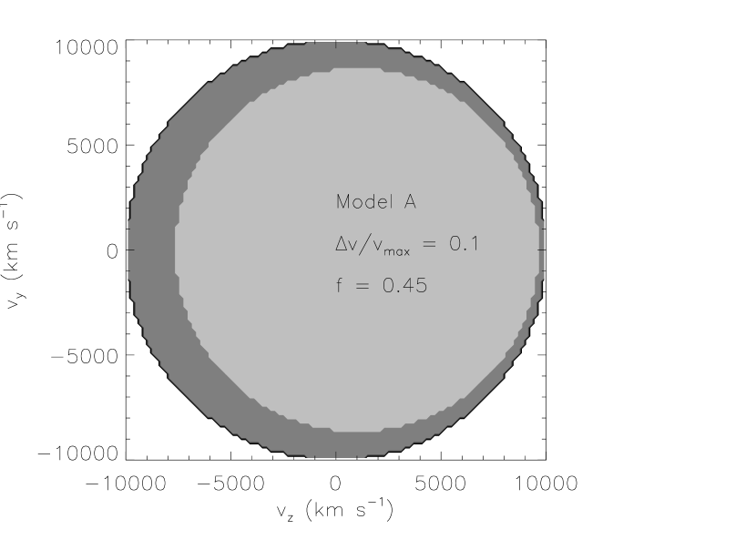
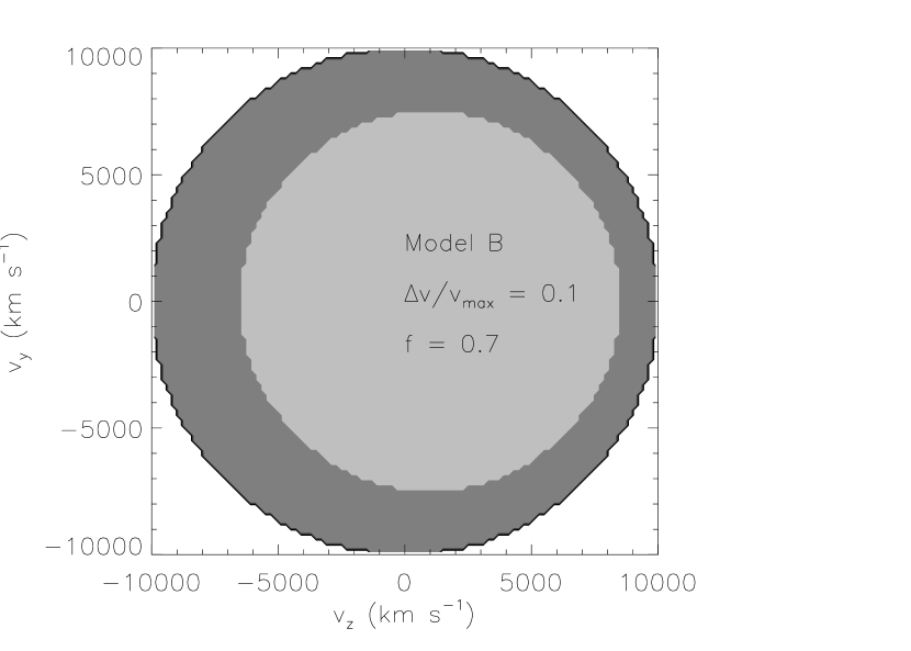
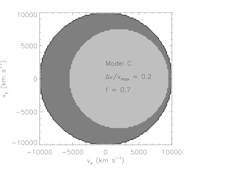
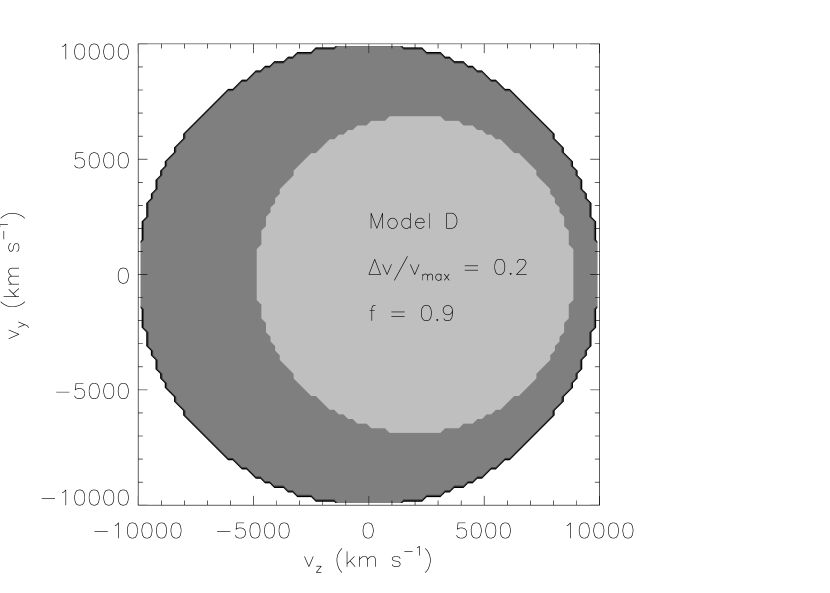
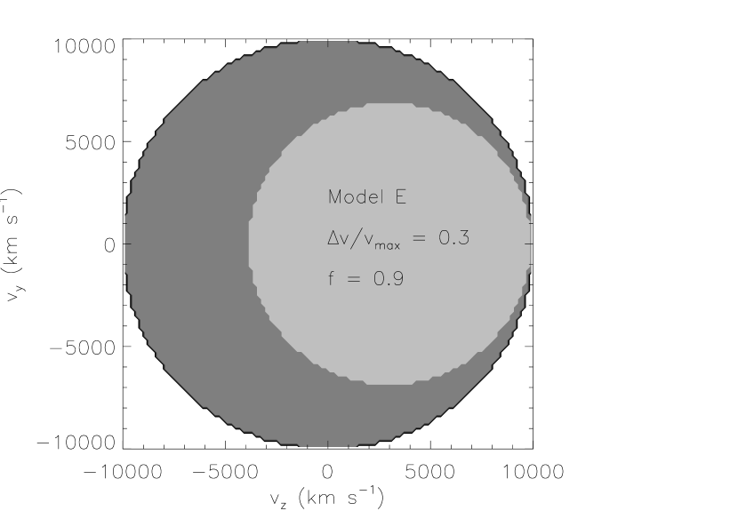
Figure 1: Slices through the y-z plane showing the distribution of ⁵⁶Ni adopted in the models. The dark grey areas indicate the regions in which there is no ⁵⁶Ni while the light grey areas are those containing a fractional mass $f$ of ⁵⁶Ni. The adopted values of $f$ are indicated in the figure. $\Delta v/v_{\mbox{\scriptsize max}}$ specifies the fractional offset in velocity of the ⁵⁶Ni centre-of-mass from the true centre-of-mass of the SN. All the models have a total mass of 1.4 M_⊙ and a total ⁵⁶Ni mass of 0.4 M_⊙. All the models are symmetric under rotation about the $z$-axis.

3 Toy models

In this section, we undertake a preliminary investigation of the effects of a lop-sided ⁵⁶Ni distribution on light curves using a set of simply-parameterized, artificial toy models. We begin by describing these models and the numerical results obtained from them (Section 3.1) and then discuss the general implications of such models (Section 3.2).

3.1 Description

To explore the role of an off-centre distribution of ⁵⁶Ni, a grid of simplistic toy models has been constructed. In each model, a total mass of 1.4 M_⊙ is adopted. The mass density is assumed to be uniform and a maximum velocity of $v_{\mbox{\scriptsize max}}=10^{4}$ km s^-1 is chosen. This simple density distribution makes it convenient to explore off-centre distributions of ⁵⁶Ni without necessitating changes in either the geometrical shape of the ⁵⁶Ni blob nor the underlying total mass distributions. In more sophisticated SN Ia models, the density distribution generally does extend to velocities greater than our adopted $v_{\mbox{\scriptsize max}}$ (e.g. in the well-known W7 model, Nomoto et al. 1984) – however, in these outer higher velocity regions, the density has typically fallen off by an order of magnitude or more compared to the inner parts which makes the outer regions relatively unimportant in grey-bolometric light curve calculations such as employed here. In particular, Pinto & Eastman (2000a) demonstrated that the light curve computed from a uniform-density spherical model with $v_{\mbox{\scriptsize max}}=10^{4}$ km s^-1 agrees very well with that obtained from the W7 model (see their figure 2).

Inside our toy SN models, the ⁵⁶Ni is also given a spherical distribution but its centre-of-mass is offset in velocity relative to that of the SN; this offset ($\Delta v$, which will generally be specified as a fraction of $v_{\mbox{\scriptsize max}}$) is one of the parameters of the models. Throughout the region which contains ⁵⁶Ni, a uniform mass-fraction $f$ is adopted – this is the second parameter of the model. In all the models the total mass of ⁵⁶Ni is fixed to 0.4 M_⊙; therefore $f$ determines the volume of the region which contains ⁵⁶Ni. In total, five models (A – E) are presented here; the structure of these models is illustrated in Figure 1. The parameters which differentiate the models ($\Delta v/v_{\mbox{\scriptsize max}}$, $f$) are indicated in the figure and also tabulated in Table 1. In all the toy models, a uniform grey-absorption cross section of 0.1 cm² g^-1 is adopted for the treatment of “bolometric” uvoir photons while the $\gamma$-ray transport and deposition is treated in detail (see Sim 2007 for a full description).

Light curves have been computed for each of the five models (A – E) for three interesting viewing directions:

1. for an observer located at a large distance along the same direction in which the Ni is displaced relative to the centre of the SN;

2. for an observer located diametrically opposite the observer in case (i);

3. for an observer lying along a line-of-sight perpendicular to the direction of displacement.

For each of these viewing angles in each of the models, the time ($t_{\rm p}$) and magnitude ($M_{\rm p}$) of maximum light have been extracted; these values are reported in Table 1.

The results in Table 1 indicate that an off-centre distribution of ⁵⁶Ni could introduce significant angular dependence in the light curve properties. In the models, the light curve peak is both earliest and brightest when viewed along the direction in which the ⁵⁶Ni is displaced. This behaviour is as expected since the mean optical depth from the ⁵⁶Ni to the edge of the ejecta is lowest in this direction; therefore, more energy packets escape more quickly. Correspondingly, when viewed from the diametrically opposite direction, the peak magnitude occurs latest and is dimmest.

It can be seen that the viewing-angle sensitivity of $M_{\rm p}$ is significantly affected by $\Delta v$ but is insensitive to the adopted value of $f$. As $\Delta v$ is increased, the variation of $M_{\rm p}$ with angle in a given model increases from about 0.5 mag for the models with $\Delta v/v_{\mbox{\scriptsize max}}=0.1$ to more than 1.5 mag for the most extreme model considered ($\Delta v/v_{\mbox{\scriptsize max}}=0.3$).

To examine the angular behaviour of the light curve properties further, one model (model C) has been studied in greater detail. For this model, light curves have been extracted for an additional eight viewing directions. These directions have been selected to give a uniform grid of viewing angles in $\cos\theta$ ($\theta$ being the angle between the line of sight direction and the direction along which the ⁵⁶Ni is displaced). Figures 2 and 3 show the variation of $M_{\rm p}$ and $t_{\rm p}$ with $\cos\theta$, respectively.

Figure 2 shows that the peak magnitude follows a near-linear dependence on $\cos\theta$. The best-fit straight line (which is drawn in the figure) is given by:

$$M_{\mbox{\scriptsize p}}=-18.67-0.52\cos\theta\;\;\;.$$ (1)

The near-linear variation with $\cos\theta$ is important since it means that the distribution of $M_{\mbox{\scriptsize p}}$ one obtains by selecting random lines-of-sight is close to a top-hat function; thus the model predicts that if one were to observe it from a random viewing direction one would be equally likely to measure any value of $M_{\mbox{\scriptsize p}}$ between about -18.2 and -19.2 with no bias towards the median.

A similarly simple relationship is apparent in Figure 3. Again, a linear fit is an adequate description; the best-fit straight line being given by

$$t_{\mbox{\scriptsize p}}=15.7-2.9\cos\theta\;\mbox{(days)}\;\;.$$ (2)

The absolute values for $t_{p}$ obtained from the toy models are generally somewhat low compared to those deduced by fitting templates to observed light curves (e.g. typically $\sim$ 19 days found in a recent study of light curves from the Supernova Legacy Survey by Conley et al. 2006). This is most likely a consequence of the simple treatment of the radiation transport which we have adopted (namely, the use of a grey, time-independent scattering cross-section per gram), but it may also be, in part, a consequence of the chosen structure of the toy models. However, a full investigation of the sensitivity of $t_{p}$ to the assumptions made in the radiation transport and the construction of the models goes beyond what we require for this study; instead we focus only on the differential effects introduced by the departures from spherical symmetry. The relative behaviour of $t_{\mbox{\scriptsize p}}$ and $M_{\mbox{\scriptsize p}}$ is discussed below.

Table 1: Light curve properties for the toy models (A – E). $\Delta v/v_{\mbox{\scriptsize max}}$ specifies the velocity offset of the ⁵⁶Ni centre-of-mass relative to the maximum velocity in the ejecta. $f$ gives the mass fraction of ⁵⁶Ni in the Ni region. $M_{\rm p}$ and $t_{\rm p}$ are the magnitude and time at which the light curve reaches its peak. The superscripts $\uparrow$, $\downarrow$ and $\perp$ indicate properties as viewed by a distant observer lying along the direction in which the ⁵⁶Ni is displaced relative to the SN centre-of-mass, anti-parallel and perpendicular to this direction, respectively. $\Delta M_{\mbox{\scriptsize p}}=M_{\mbox{\scriptsize p}}^{\downarrow}-M_{\mbox{\scriptsize p}}^{\uparrow}$ is the range in $\Delta M_{\mbox{\scriptsize p}}$ as a function of viewing angle for the model.

Model	$\Delta v/v_{\mbox{\scriptsize max}}$	$f$	$M_{\mbox{\scriptsize p}}^{\uparrow}$	$t_{\mbox{\scriptsize p}}^{\uparrow}$	$M_{\mbox{\scriptsize p}}^{\downarrow}$	$t_{\mbox{\scriptsize p}}^{\downarrow}$	$M_{\mbox{\scriptsize p}}^{\perp}$	$t_{\mbox{\scriptsize p}}^{\perp}$	$\Delta M_{\mbox{\scriptsize p}}$
				days		days		days
A	0.1	0.45	-19.00	12.0	-18.47	15.2	-18.71	13.5	0.53
B	0.1	0.70	-18.95	13.9	-18.43	16.4	-18.69	15.6	0.52
C	0.2	0.70	-19.21	12.7	-18.18	18.1	-18.67	15.7	1.03
D	0.2	0.90	-19.19	13.5	-18.14	18.7	-18.64	16.1	1.05
E	0.3	0.90	-19.43	12.0	-17.85	20.3	-18.59	15.9	1.58

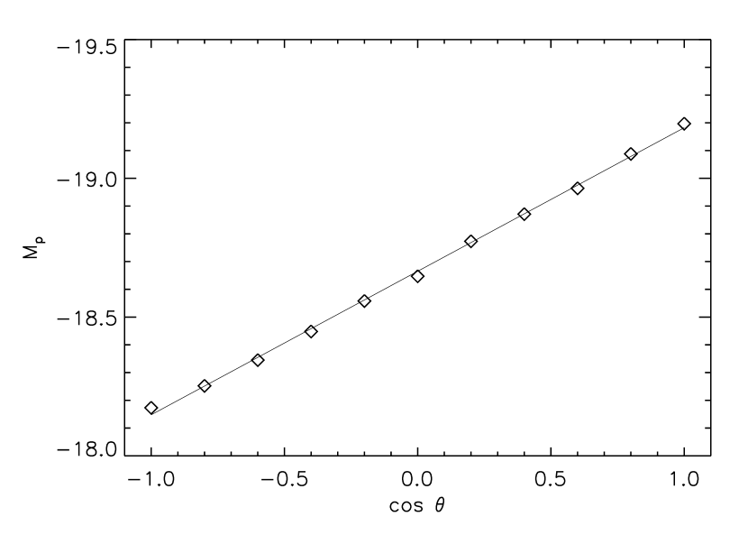
Figure 2: The peak bolometric magnitude ($M_{\mbox{\scriptsize p}}$) as a function of the viewing direction ($\theta$) for light curves computed with model C (shown as diamonds). The solid line is the linear fit to the results (see text).

Figure 3: The time at which peak magnitude occurs ($t_{\mbox{\scriptsize p}}$) as a function of the viewing direction ($\theta$) for light curves computed with model C (shown as diamonds). The solid line is the linear fit to the results (see text).

3.2 Discussion of the toy models and Arnett’s Rule

The results obtained with the toy models described above can be used to gain some insight into how observable light curve properties behave. In Figure 4, the values of $M_{\mbox{\scriptsize p}}$ are plotted against $t_{\mbox{\scriptsize p}}$ for all the light curves summarised in Table 1. In addition, the grid of light curves computed to map out the angle dependence with Model C are also represented (eight additional points). We emphasise that, since all the models considered adopt the same total mass of ⁵⁶Ni, the variation in $M_{\rm p}$ amongst the different points is entirely the result of the differences in the distribution of Ni with velocity. Since there is no compelling reason to suppose that all observed SN Ia synthesise the same total mass of ⁵⁶Ni – indeed, to the contrary, the total mass of ⁵⁶Ni is likely a dominant parameter in distinguishing SN Ia – our results (Figure 4) cannot be regarded as predictions or a model for the directly observed distribution of SN Ia light curve parameters. Instead, they should be correctly interpreted in terms of a possible differential effect which is sensitive to the observer line-of-sight and which would appear in observed distributions superimposed upon other effects whose origins may lie in the underlying distributions of SN Ia explosion properties.

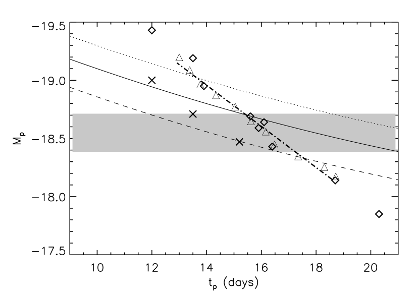
Figure 4: The peak magnitude ($M_{\mbox{\scriptsize p}}$) versus the light curve rise time ($t_{\mbox{\scriptsize p}}$) from the toy models. There are in total twenty-three light curves represented in the figure. The triangles represent the eleven light curves computed from Model C (as discussed in Section 3.1, these have been calculated on a uniform grid in $\cos\theta$-space) and the heavy dot-dashed line is the description of the Model C results obtained by combining the fits given in equations 1 and 2. The crosses represent the light curves computed from Model A while the diamond symbols show those from Models B, D and E; there are three viewing angles (parallel, perpendicular and anti-parallel to the direction of Ni-offset) per model (the numerical values are given in Table 1). The three curves – dashed, solid and dotted lines – show the expected Arnett relation obtained from equations 3 and 4 adopting $\alpha=0.8$, $1.0$ and $1.2$, respectively. The shaded grey-region indicates the range of values for $M_{\mbox{\scriptsize p}}$ predicted following Stritzinger & Leibundgut (2005) for the ⁵⁶Ni mass adopted in the toy models.

As mentioned in Section 3.1, the range of $M_{\mbox{\scriptsize p}}$ obtained from the grid of models is very wide, spanning more than 1.5 mag. This illustrates that the effects of a lop-sided Ni distribution could, in principle, be very significant at the precision level set by contemporary observational data (e.g. in a sample of SNe for which bolometric peak magnitudes are available, as presented by Stritzinger & Leibundgut 2005, the error estimates typically correspond to 10 – 15 per cent in flux). The scale of the effects is broadly comparable to those established for other models involving departures from sphericity. For example, Höflich (1991) investigated some observational consequences of ellipsoidal SN ejecta and showed that for quite modest departures from sphericity (axis ratios in the range 0.9 to 1.2), one finds a viewing angle dependence of the peak brightness on the scale of tenths of a magnitude (see also Howell et al. 2001 and Wang et al. 2003 for motivation of such a model in the context of spectropolarimetric observations). As one would expect, even greater angular variations – comparable to those obtained here – can be obtained from ellipsoidal models with more extreme axis ratios (Sim, 2007). Similar scales of light curve angular dependence (up to $\sim 0.25$ mag) were also found by Kasen et al. (2004) in a study of a SN model with a geometric “hole” in the ejecta and by Kasen & Plewa (2006) in a very recent study of a 2D GCD model.

We note that the angular variation is so large that one can likely rule out the more extreme models (models C, D and E) as being representative of typical SNe conditions – this follows from the observed tightness of the correlation in the plot of bolometric flux versus recession velocity for nearby SNe Ia (the “Hubble diagram”; see e.g. Stritzinger & Leibundgut 2005). However, these models do show that it is possible to arrange extreme geometries that could produce substantial deviations from the mean and provide one possible explanation for some apparently anomalous events (Hillebrandt et al., 2007).

Since both $M_{\rm p}$ and $t_{\rm p}$ are simple functions of the viewing angle (equations 1 and 2), it follows that there is an equally simple relationship between these two quantities for a given model, as can be seen in Figure 4. For the models with moderate to large values of $f$ (Models B – E), the points are all fairly close to following the same line in the $M_{\rm p}$-$t_{\rm p}$ plane. Thus, from these models alone one might hope that combined measurements of both $M_{\rm p}$ and $t_{\rm p}$ could be used to extract the true luminosity despite the effect of viewing angle. However, the points obtained with model A lie significantly below this line, showing that the relationship is not universal.

A point of particular interest relates to the interpretation of Arnett’s Rule (Arnett, 1982) which is commonly used to estimate Ni masses in studies of SNe Ia light curves (e.g. Arnett et al. 1985; Branch 1992; Stritzinger & Leibundgut 2005; Stritzinger et al. 2006a; Stritzinger et al. 2006b; Howell et al. 2006). Arnett’s Rule states that at maximum light, the luminosity roughly balances the instantaneous rate of energy generation in the SN. Adopting the convenient notation of Branch (1992) this relation is stated as

$$L^{\mbox{\scriptsize p}}=\alpha R(t_{\mbox{\scriptsize p}})M_{\mbox{\scriptsize Ni}}$$ (3)

where $L^{\mbox{\scriptsize p}}$ is the peak luminosity, $R(t_{\mbox{\scriptsize p}})$ is the rate of energy generation at the time of maximum light ($t_{\mbox{\scriptsize p}}$) and $M_{\mbox{\scriptsize Ni}}$ is the total mass of ⁵⁶Ni. The proportionality factor, $\alpha$, is expected to be of order unity. $R(t)$ is given by

$$R(t)=[6.41\;e^{-t/8.8}+1.34\;e^{-t/113.7}]10^{43}\;\;\mbox{ergs s${}^{-1}$ M${}_{\odot}^{-1}$}$$ (4)

where $t$ is measured in days. The numerical coefficients have been computed using the lifetimes and decay energies from Ambwani & Sutherland (1988).

It is well-known from several previous studies that Arnett’s Rule can usually be used to derive a reasonable estimate for $M_{\mbox{\scriptsize Ni}}$ from the light curve. However, it is not strictly obeyed, particularly if there is Ni present in the outermost regions of the SN ejecta, as discussed by Pinto & Eastman (2000a). Since Arnett’s Rule relates only global quantities, for any class of SN model in which a viewing angle dependence of the flux appears (including, but not limited to, the off-centre models discussed here), an attempt to measure the nickel-mass via Arnett’s Rule must introduce a systematic error which depends upon the direction of observation. In this section, we will use the toy models to investigate how this systematic would behave if real SNe (or at least a subset of them) were to harbour lop-sided distributions of ⁵⁶Ni.

First we consider the case where a Ni mass is deduced by the application of Arnett’s Rule (with a chosen value, or range of values, for $\alpha$) to direct measurements of the observed peak magnitude and time of maximum light. To elucidate this case, we over-plot in Figure 4 the curves obtained by combining equations 3 and 4 for three different values of $\alpha$ (0.8, 1.0, 1.2). It comes as no surprise that Arnett’s Rule with a fixed value of $\alpha$ does not describe the co-dependence of $M_{\rm p}$ and $t_{\rm p}$ obtained from the models – the Rule is concerned with relating global properties of different SNe, not the detailed angular dependence within single objects. However, the correlation of $M_{\rm p}$ and $t_{\rm p}$ deriving from Arnett’s Rule is in the same sense as that obtained from the models. This helps to suppress the systematic error one would introduce with an unknown viewing angle; for the more moderate models (A and B), the systematic error introduced would be only around 0.15 to 0.2 mag. In exceptional cases, however, a much larger systematic error of up to about 0.5 mag is possible for the adopted Ni mass.

Secondly, we consider the case where reliable measurement of $t_{\rm p}$ has not been possible so that an estimate of $M_{\mbox{\scriptsize Ni}}$ must be obtained from $M_{\rm p}$ alone. Adopting the relationship discussed by Stritzinger & Leibundgut (2005) (their equation 7 which is derived from Arnett’s Rule and an empirically motivated assumption for the value of $t_{\rm p}$), leads to an expected value of $M_{\rm p}=-18.56\pm 0.16$ mag for $M_{\mbox{\scriptsize Ni}}=0.4$ M_⊙. This range of $M_{\rm p}$ is indicated in Figure 4 by the grey shaded region; thus all the points which fall within this band are consistent with the Stritzinger & Leibundgut (2005) relationship. For all the models considered, a significant fraction of the possible viewing directions lead to light curves which lie outside the range. Thus, if the range of light curve properties produced by the models were representative of those from real SNe, using that relationship between $M_{\rm p}$ and $M_{\mbox{\scriptsize Ni}}$ in the analysis of a sample of observed light curves could lead one to infer a wider spread of nickel masses than required.

The toy models have demonstrated that it is possible to construct very simplistic scenarios in which a lop-sided distribution of ⁵⁶Ni can introduce significant angular dependence in the emergent radiation. The scale of the variation is comparable to that introduced by other types of departure from spherical symmetry (Höflich 1991; Kasen et al. 2004) and can be comparable to, or larger than, typical observational uncertainties. However, the toy models are very simplistic and are derived with no reference to realistic explosion physics. Therefore, they merely illustrate possible effects and one must appeal to 3D explosion models to judge whether such effects are likely to have a part to play in reality. The remainder of this paper is concerned with the analysis of results from one such model.

4 A 3D explosion model

4.1 The model

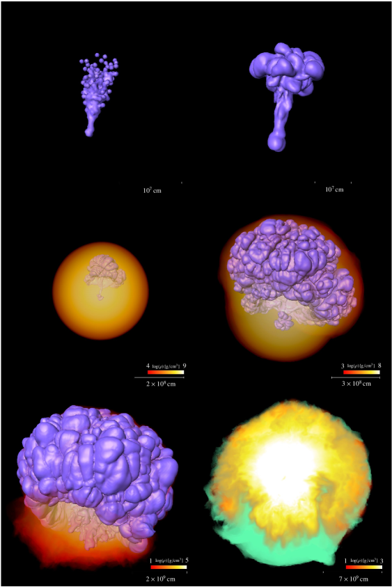
Figure 5: Evolution of the 3D simulation 3T2d200. The initial flame configuration is shown in the upper left panel; the blue isosurface corresponds to the zero level set associated with the thermonuclear flame. The following four panels ($t=0.2\,\mathrm{s}$, $t=0.4\,\mathrm{s}$, $t=1.0\,\mathrm{s}$, and $t=3.0\,\mathrm{s}$; left to right, top to bottom) illustrate the evolution of the model. Again, the blue isosurface corresponds to the zero level set associated with the flame where burning is active and gives an approximate interface between fuel and ashes where the densities are below the burning threshold ($10^{7}\,\mathrm{g}\,\mathrm{cm}^{-3}$). The star is indicated in some of the figures by the volume-rendering of the density (red through yellow to white). The lower right image illustrates the composition of the ejecta (the front hemisphere is cut away) at the end of the simulation ($t=10.0\,\mathrm{s}$). Unburned material (carbon and oxygen) is shown in green and the white/yellow/orange volume-rendering corresponds to the density of the iron group elements.

The 3D explosion simulation 3T2d200 described by Röpke et al. (2007) has been used as the basis for a model to explore the effects of an off-centre ⁵⁶Ni distribution in a realistic case. This simulation followed the flame evolution when ignited in a lop-sided teardrop-like shape (upper left panel of Figure 5). Such an ignition configuration is motivated by recent studies of the pre-ignition convective burning phase (Kuhlen et al., 2006), which suggest that the flow pattern is dominated by a dipole at this stage. A consequence could be a lop-sided ignition as adopted here, where the majority of ignition kernels are located on one side of the star but with a slight over-shooting across the centre. In this case, the flame propagates in both directions, subject to buoyancy instabilities and accelerated by turbulence. One side of the flame structure, however, remains dominant (see the top left panel in Figure 5). Although the ash bubble on this side of the star starts to sweep around the core (similar to what has been described by Plewa et al. 2004), it does not collide on the far side (see the panels in the second row of Figure 5) because the energy generated by nuclear burning is sufficient to gravitationally unbind the star and expand it before a collision occurs. The lower left panel of Figure 5 shows the end-stage of this evolution; subsequently the expansion is approaching homology. The composition of the ejecta is illustrated in the lower right panel of Figure 5, showing a pronounced asymmetric bubble of iron-group elements. The simulation was carried out on a 512³ cells moving Cartesian computational grid (Röpke, 2005).

The model used here for radiation transport adopts a uniform Cartesian grid with 128³ cells. The total mass density and the mass fraction of Fe-group elements in each cell was obtained directly from the hydrodynamic simulation by combining sets of 4³ cells from the original 512³ grid. The cell properties were extracted from the latest time to which the hydrodynamics calculation was followed ($\sim$10s). For times beyond this point, including the entirety of the time for which the radiative transfer is followed, the ejecta are assumed to be in homologous expansion.

Since the hydrodynamical results did not provide detailed information on the composition of the ash material, it has been assumed that initially all the Fe-group mass was composed of ⁵⁶Ni; this gives a total of 0.448 M_⊙ of ⁵⁶Ni. Since this investigation is concerned with the viewing-direction dependence of the light curve, this assumption will not significantly affect our conclusions – a lower mass fraction of ⁵⁶Ni in the ash would merely reduce the total luminosity; it would only affect the angle-dependence if the mass fraction were to vary significantly with position; whether or not this could be the case must await more detailed nucleosynthesis modelling in 3D.

4.2 Treatment of opacity

In the calculations using the 3T2d200 model, a slightly more sophisticated treatment of uvoir opacity is employed than the uniform grey cross-section adopted for the toy models. Following (Mazzali & Podsiadlowski, 2006), an opacity which depends on composition is adopted, the particular form used here being

$$\sigma=0.26\;(0.9X_{\mbox{\scriptsize Fe-grp}}+0.1)\;\mbox{cm${}^{2}$~{}g${}^{-1}$}$$ (5)

where $X_{\mbox{\scriptsize Fe-grp}}$ is the mass-fraction of iron-group elements, which varies throughout the model. This simple parameterisation takes advantage of the basic compositional information available directly from the hydrodynamics calculation (namely the mass-fraction of heavy elements) to attempt to account for the dominance of the iron-group elements in providing opacity.

As has been discussed elsewhere (e.g. see Pauldrach et al. 1996 and Pinto & Eastman 2000b for in-depth discussion or Sim 2007 for comments in the context of the code used here), the uvoir-opacity in SN ejecta is mostly dominated by spectral lines. Given this, the grey-approximation adopted here is not valid in detail – in particular, it cannot account for the process of photon redistribution in frequency-space which allows photons to escape the ejecta by down-scattering into frequency regimes in which the density of spectral lines is low. This process effectively limits the maximum trapping any photon can undergo, an effect which is most relevant at the earliest times. For this reason, the grey-approximation may overestimate the dependence of radiative transfer effects on geometry. Nevertheless, the grey approximation is retained here since it dramatically reduces the computational demands of the radiation transfer calculations compared to a full non-LTE calculation. Despite this approximation, the computations can be expected to correctly identify the sense in which purely geometrical effects will act and to give a simple estimate, or at least a reliable limit, for their scale.

Of course, fully 3D, non-LTE, non-grey calculations are necessary to quantify the effects rigorously – however, to utilise this level of sophistication in the radiative transfer fully, one would also require more complete information on the detailed nucleosynthesis products and the ultimate evolution toward homology than is presently available for the 3T2d200 model. Fortunately, as discussed by Lucy (2005), the Monte Carlo radiative transfer method is well-suited to incorporating more advanced treatments of microphysics and thus there is great promise for more detailed treatments when merited (see, e.g. Kasen et al. 2006, Kasen & Plewa 2006).

4.3 Results obtained with the explosion model

We begin by presenting and describing the light curve properties obtained from the 3T2d200 model. Figure 6 shows light curves obtained for the special viewing directions parallel and anti-parallel to the vector connecting the centre-of-mass of the ejecta and the centre-of-mass of the ⁵⁶Ni; throughout the discussion we denote this vector $n$ – note that $n$ is nearly, but not quite, parallel to $\hat{z}$.

Figure 6: Computed light curves from the 3T2d200 model (Röpke et al., 2007). The dashed line shows the angle-averaged light curve. The heavily and lightly drawn histograms show, respectively, the light curve as seen by distant observers who lie along the direction-vectors $\hat{n}$ and $-\hat{n}$. $\hat{n}$ is the unit-vector which points from the centre-of-mass of the ejecta to the centre-of-mass of ash material.

We see from the figure that there are differences in the light curve properties as seen from these two directions – in agreement with the results from the toy models, the scale of the effect is significant compared to typical observational accuracy ($\leq 0.1$ mag). Also in accordance with the results obtained in Section 3.1, the light curve is brightest and rises to maximum fastest when viewed down $n$. In contrast to the toy-model results, however, the anti-parallel direction does not show the dimmest light curve for the 3D model – this is a consequence of the more complex distribution of ash material which determines both the location of energy generation (⁵⁶Ni) and the distribution of opacity (via the dependence on $X_{\mbox{\scriptsize Fe-grp}}$ in equation 5). As might be anticipated from Figure 5 (lower panels), the dimmest light curves are actually seen by observers whose line-of-sight is nearly perpendicular to $n$ (see below).

While the light curves shown in Figure 6 indicate that it is possible to see significant differences in the peak magnitude as a function of direction, it is important to consider how probable a randomly aligned observer is to see a given range of light curve parameters. To this end, a grid of 100 viewing directions (evenly spaced in solid angle), has been employed to map out the angular distribution of the light curve properties. In Figure 7 the peak magnitudes are shown for this grid of directions as a function of the polar angle, $\theta$, ($\theta$ being the angle between the $z$-axis of the model and the observer’s line-of-sight). There is clearly a net trend in the variation of $M_{\rm p}$ with $\theta$; for large values of $\cos\theta$ the mean trend is very similar to that found in the toy models. But, as noted above, owing to the complex distribution of ash material, a much weaker trend is revealed in the region where $\cos\theta<0$.

Figure 7: The peak magnitude as a function of the spherical polar angle $\theta$ as obtained with the 3T2d200 model. For each value of $\theta$ there are 10 points, each representing a different azimuthal angle, $\phi$.

The grid of light curves as a function of viewing directions can be used to determine the probability distribution for the peak magnitude. This has been done and the resulting cumulative probability distribution is shown in Figure 8.

Figure 8: The peak-magnitude cumulative probability distribution function – the probability that the obtained value of $M_{\rm p}$ is less than $m$ – as obtained from the 3T2d200 model. The median value is -18.67 (dashed line).

Although more complex in detail, the probability distribution function (pdf) obtained shares most of the important properties suggested by the toy models; namely, it is fairly wide (spanning $\sim$ 0.5 mag) and the probability is not strongly concentrated around the median (for example, fully one quarter of the directions give peak magnitudes that are brighter than the median by at least 0.1 mag). An important difference from the pdf implied by the toy models is a distinct asymmetry (as could be anticipated from Figure 7) – there is a probability tail extending to brighter magnitudes meaning that one may see larger differences on the bright side than on the dim side of the median. The probability distribution for $M_{\rm p}$ will be used in Section 5.2 to quantify the relevance of this work to the interpretation of the local Hubble diagram.

For completeness, Figure 9 shows the range of light-curve rise times with viewing direction. As with the toys models, it can be seen that there is significant diversity in the rise time and that it tends to be shortest when viewing down $n$ (i.e. close to $\theta=0$) and longest when viewing closer to $-n$ (i.e. $\theta\sim\pi$). In the next section, we examine the relationship between rise time and peak magnitude in some detail.

Figure 9: As for Figure 7 but showing the time at which maximum light occurs.

5 Implications of the 3D calculations

We now consider some ramifications of the results obtained from the 3D model that has been discussed in Section 4.

5.1 Arnett’s Rule and observational estimates of Ni masses

In Section 3.2 we used the toy models to investigate the possible systematic effects of an off-centre explosion on the inference of Ni masses. Here, we extend that discussion using the results obtained with the 3T2d200 explosion model.

Figure 10 shows the peak magnitude versus the time of maximum light for the set of 100 light curves obtained for different viewing directions in the 3T2d200 model. As in Figure 4, curves are over-plotted to indicate the trends predicted by equations 3 and 4. Similarly, the grey band indicates the region in which the computed values of $M_{\rm p}$ are consistent with the relationship presented by (Stritzinger & Leibundgut, 2005).

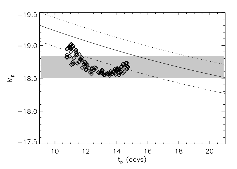
Figure 10: The peak magnitude ($M_{\mbox{\scriptsize p}}$) versus the light curve rise time ($t_{\mbox{\scriptsize p}}$) from the 3T2d200 model (Röpke et al. 2006). The opacity depends on composition via equation 5. The three curves – dashed, solid and dotted lines – show the expected Arnett relation obtained from equations 3 and 4 adopting $\alpha=0.8$, $1.0$ and $1.2$, respectively. The shaded grey-region indicates the range of values for $M_{\mbox{\scriptsize p}}$ predicted following Stritzinger & Leibundgut (2005) for a ⁵⁶Ni mass of 0.488 M_⊙.

The figure reveals several interesting phenomena. Amongst the highest luminosity and fastest rise-time light curves there remains a trend which is reminiscent of what was suggested by the toy models (Figure 4). However, this trend does not continue through the light curves with longer rise times; instead, the trend first flattens and then turns over – a result of the non-linear angular dependence of $M_{\rm p}$ as shown in Figure 7. This has the consequence that, as the viewing angle is varied, the light curve properties stay fairly close to those inferred via Arnett’s Rule (with $\alpha\sim 0.8$) but with systematic variation of around $\sim 0.2$ mag ($\sim 20$ per cent in luminosity).

The value for the peak bolometric magnitude obtained using the model ⁵⁶Ni mass and following Stritzinger & Leibundgut (2005) is very close to the median of the peak magnitude obtained amongst the different viewing angles. The error range which they suggest – based on an estimated range of possible light curve rise times – happens to be rather close to encompassing the range of peak magnitudes obtained from the model. However, there are a moderate number of model light curves which lie outside this range, all of which are brighter than the Stritzinger & Leibundgut (2005) relation would anticipate.

Thus we conclude that the calculations involving the fully 3D model support the primary result obtained with the toy models, namely that observationally significant systematic errors can be introduced via viewing angle effects in off-centre explosions. The particular model used here has a maximum spread in $M_{\rm p}$ of about 0.5 mag, which is comparable to that obtained with toy model A. However, the particularly simple, linear dependence of $M_{\rm p}$ with $\cos\theta$ (see Figure 2) is not preserved in the 3D model.

5.2 Scatter in the local Hubble diagram

In this section we investigate what effect the predicted viewing angle dependence would have on the observed relationship between peak magnitude and recession velocity for SNe Ia in the Hubble flow.

Assuming that the properties of the 3T2d200 model (Figure 7) are representative for a population of SNe Ia, the viewing-angle dependence of the bolometric light curve would lead to a scatter about the mean relationship between peak flux and recession velocity. To quantify this effect, we have used the probability distribution of the peak magnitude (Figure 8) to map the region of the local Hubble diagram that would be occupied by a hypothetical population of SNe Ia which are in the Hubble flow and which have properties as predicted by the 3T2d200 model. This region is indicated by the shaded area in Figure 11. Over-plotted are lines which show contours of the probability distribution; these contours are slightly concentrated toward the fainter side owing to the asymmetry of the probability distribution (see Section 4.3).

In constructing the Hubble diagram (via equation 10 of Stritzinger & Leibundgut 2005) we have adopted a value for the Hubble parameter, $H_{0}=85$ km s^-1 Mpc^-1. This value is the one that Stritzinger & Leibundgut (2005) obtain from their analysis using a typical ⁵⁶Ni mass of 0.42 M_⊙; as they discuss, this value for $H_{0}$ is unusually large and most likely a result of a net under-prediction for the amount of ⁵⁶Ni produced in the pure deflagration explosion models that they discuss. Although this is clearly an important issue, it is not of relevance to our discussion of scatter in the Hubble diagram since the effect of changing the adopted value of $H_{0}$ amounts to only a fixed offset in the ordinate of Figure 11.

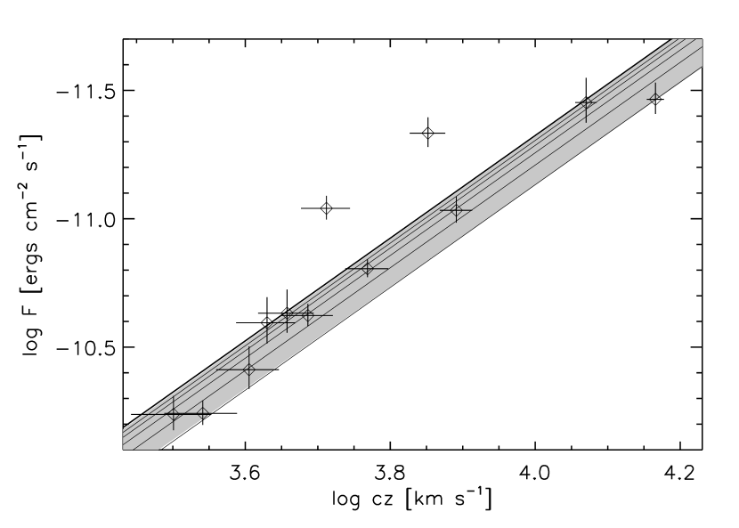
Figure 11: The peak uvoir flux ($F$) versus recession velocity ($cz$) for SNe Ia in the local Universe. The grey shaded area indicates the region which would be populated by a multitude of 3T2d200 SNe in the Hubble flow having random orientations relative to the observer line-of-sight. The solid lines are drawn to delineate equal intervals of the underlying probability distribution for $M_{\rm p}$ (they show 20 per cent intervals). The twelve data points which are over-plotted are those for the SNe Ia discussed by Stritzinger & Leibundgut (2005).

For comparison, the flux and recession velocities for the sample of twelve local SNe Ia which was assembled and used by Stritzinger & Leibundgut (2005) are also shown in the figure. Although relatively small compared to data sets obtained from the large scale supernova surveys, the Stritzinger & Leibundgut (2005) sample is ideally-suited for comparison with our results since the objects they include have been selected on the basis of having sufficiently large wavelength coverage that the bolometric peak magnitude is well-determined observationally; this is important since our calculations do not distinguish between different photometric bands. Also, the fluxes tabulated by Stritzinger & Leibundgut (2005) have not been normalised or modified using any empirically motivated stretch factors or light curve shape correlations. Since we do not compute band-limited light curves, we cannot use the standard empirical correlations quantitatively (e.g. the Phillips 1993 relation) to renormalise our calculations. Therefore, for quantitative comparison of like with like, we require the distribution of observed bolometric fluxes corrected only for observational effects such as reddening.

Figure 11 clearly demonstrates two important points which we now discuss in turn. First, it shows that the viewing angle variation predicted by the 3T2d200 model does not substantially exceed the scale of scatter in the observed Hubble diagram. Therefore, one cannot rule out the 3T2d200 model as representative of a typical SN Ia by arguing that its asphericity is inconsistent with the observed narrowness of the Hubble-diagram correlation. This is in contrast to the more extreme toy models (see Section 3.2) which could be excluded by this argument directly.

Secondly, it can also be seen that the angular variations in the peak magnitude are on the correct scale to account for the observed dispersion about the mean relation. Thus it is probable that orientation effects in aspherical SNe Ia could contribute significantly to the dispersion in the Hubble diagram. Indeed we conclude that, excluding the two apparently sub-luminous objects (SN1992bo and SN1993H), the width of the distribution of bolometric magnitudes in the sample of well-observed objects selected by Stritzinger & Leibundgut (2005) can be explained fully by the viewing angle effects predicted from the 3T2d200 model without the need to invoke any other systematic or random uncertainty.

If the scatter found in the bolometric model light curves translates into a similar scatter in band limited light curves, this effect would have important implications for the use of SNe Ia as standard candles: as a real physical effect which is dependent on the explosion mechanism, it must be understood and cannot be eliminated as a source of dispersion by improved observational statistics or measurements alone. In addition, the finding that the probability distribution is not symmetric around the mean (cf. Figure 8) could potentially introduce an additional bias in the interpretation of observed SN samples – if a significant fraction of the observed SN Ia sample has properties similar to the ones found in this model, the probability to find objects that are fainter than the mean may be somewhat larger than finding ones brighter than the mean.

The commonly used methods to correct the peak magnitude based on the shape of the light curve in certain filter bands (e.g., Phillips 1993, Riess et al. 1996) are not expected to account for the orientation effect fully. The calibration methods address a scatter in the band-limited peak flux which is most likely introduced by different degrees of nuclear burning and mixing which affect the emerging radiation in specific filter bands (Höflich et al. 1995; Pinto & Eastman 2001; Mazzali et al. 2001; Kasen & Woosley 2007) through the resulting variation in the composition and thermal structure of the ejecta. Because it is unlikely that the orientation effects follow the same correlation, it is expected that these two sources of scatter will be superimposed in the distribution of observed peak magnitudes in particular photometric bands.

It is conceivable that a relation between observables can be found that allows a correction following the spirit of the Phillips relation. However, the calculations presented here are not suitable to address this question because band-limited light curves, and likely also simulated spectra for the 3D model, are required to consider this point in detail. Knowing how the orientation effect affects the band limited light curves would also enable us to analyse the much larger data sets that are available for SNe Ia observed in specific wavelength bands to estimate the significance of asphericity in the observed objects.

6 Summary

Motivated by recent explosion models involving off-centre ignition in SNe Ia, we have investigated the possible range of effects of a lop-sided distribution of nuclear ash on bolometric light curves for such objects.

By studying results from both a grid of simple toy models and one real explosion model, we find that off-centre distributions of material which has undergone nuclear burning are likely to leave detectable imprints on observed light curves. An angular dependence of the light curve peak brightness is introduced – based on the models considered, the scale of this effect can be readily $\sim 0.2$ mag and conceivably much greater under extreme circumstances.

This effect is large enough to have ramifications for the interpretation of the diversity in observed SN Ia properties and we have shown that the explosion model which we considered (Röpke et al., 2007) already predicts sufficient viewing-angle sensitivity to explain much of the typical scatter in a sample of objects with well-observed bolometric properties (Stritzinger & Leibundgut, 2005).

In view of the potential observational significance, further study of this class of explosion model is required. Investigation of viewing angle effects across a more diverse range of observable quantities is warranted (i.e. photometric band-limited light curves and, ultimately, spectra) to establish whether and by what means such effects may be observationally distinguished from other factors which determine light curve properties (e.g. the total ⁵⁶Ni mass). Furthermore, a wider investigation of the possible extent and frequency of off-centre ignition in explosion models is needed so that the likelihood for occurrence of such events – and therefore the potentially important systematics they may introduce to statistical analysis of the SN Ia sample – can be quantified.

References

- Ambwani & Sutherland (1988) Ambwani K., Sutherland P., 1988, ApJ, 325, 820
- Arnett (1982) Arnett W. D., 1982, ApJ, 253, 785
- Arnett et al. (1985) Arnett W. D., Branch D., Wheeler J. C., 1985, Nature, 314, 337
- Astier et al. (2006) Astier P. et al., 2006, A&A, 447, 31
- Blinnikov et al. (2006) Blinnikov S. I., Röpke F. K., Sorokina E. I., Gieseler M., Reinecke M., Travaglio C., Hillebrandt W., Stritzinger M., 2006, A&A, 453, 229
- Branch (1992) Branch D., 1992, ApJ, 392, 35
- Calder et al. (2004) Calder A. C., Plewa T., Vladimirova N., Lamb D. Q., Truran J. W., 2004, astro-ph/0405162
- Cappellaro et al. (1997) Cappellaro E., Mazzali P. A., Benetti S., Danziger I. J., Turatto M., della Valle M., Patat F., 1997, A&A, 328, 203
- Clocchiatti et al. (2006) Clocchiatti A. et al., 2006, ApJ, 642, 1
- Conley et al. (2006) Conley A. et al., 2006, AJ, 132, 1707
- Gamezo et al. (2003) Gamezo V. N., Khokhlov A. M., Oran E. S., Chtchelkanova A. Y., Rosenberg R. O., 2003, Science, 299, 77
- Hillebrandt & Niemeyer (2000) Hillebrandt W., Niemeyer J. C., 2000, Ann. Rev. Astron. Astrophys., 38, 191
- Hillebrandt et al. (2007) Hillebrandt W., Sim S. A., Röpke F. K., 2007, 465, L17
- Höflich (1991) Höflich P., 1991, A&A, 246, 481
- Höflich et al. (1995) Höflich P., Khokhlov A. M., Wheeler J. C., 1995, ApJ, 444, 831
- Höflich & Stein (2002) Höflich P., Stein J., 2002, ApJ, 568, 779
- Howell et al. (2001) Howell D. A., Höflich P., Wang L., Wheeler J. C., 2001, ApJ, 556, 302
- Howell et al. (2006) Howell D. A. et al., 2006, Nature, 443, 308
- Kasen et al. (2004) Kasen D., Nugent P., Thomas R. C., Wang L., 2004, ApJ, 610, 876
- Kasen & Plewa (2006) Kasen D., Plewa T., 2006, ApJ submitted (astro-ph/0612198)
- Kasen et al. (2006) Kasen D., Thomas R. C., Nugent P., 2006, ApJ, 651, 366
- Kasen & Woosley (2007) Kasen D., Woosley S. E., 2007, ApJ, 656, 661
- Khokhlov (1991) Khokhlov A. M., 1991, A&A, 245, 114
- Kozma et al. (2005) Kozma C., Fransson C., Hillebrandt W., Travaglio C., Sollerman J., Reinecke M., Röpke F. K., Spyromilio J., 2005, A&A, 437, 983
- Kuhlen et al. (2006) Kuhlen M., Woosley S. E., Glatzmaier G. A., 2006, ApJ, 640, 407
- Lucy (1999) Lucy L. B., 1999, A&A, 345, 211
- Lucy (2005) Lucy L. B., 2005, A&A, 429, 19
- Maeda et al. (2006) Maeda K., Mazzali P. A., Nomoto K., 2006, ApJ, 645, 1331
- Mazzali et al. (2001) Mazzali P. A., Nomoto K., Cappellaro E., Nakamura T., Umeda H., Iwamoto K., 2001, ApJ, 547, 988
- Mazzali & Podsiadlowski (2006) Mazzali P. A., Podsiadlowski P., 2006, MNRAS, 369, L19
- Mazzali et al. (2007) Mazzali P. A., Röpke F. K., Benetti S., Hillebrandt W., 2007, Science, 315, 825
- Niemeyer & Woosley (1997) Niemeyer J. C., Woosley S. E., 1997, ApJ, 475, 740
- Nomoto et al. (1984) Nomoto K., Thielemann F.-K., Yokoi K., 1984, ApJ, 286, 644
- Pauldrach et al. (1996) Pauldrach A. W. A., Duschinger M., Mazzali P. A., Puls J., Lennon M., Miller D. L., 1996, A&A, 312, 525
- Perlmutter et al. (1999) Perlmutter S. et al., 1999, ApJ, 517, 565
- Phillips (1993) Phillips M. M., 1993, ApJL, 413, L105
- Pinto & Eastman (2000a) Pinto P. A., Eastman R. G., 2000a, ApJ, 530, 744
- Pinto & Eastman (2000b) Pinto P. A., Eastman R. G., 2000b, ApJ, 530, 757
- Pinto & Eastman (2001) Pinto P. A., Eastman R. G., 2001, New Astronomy, 6, 307
- Plewa et al. (2004) Plewa T., Calder A. C., Lamb D. Q., 2004, ApJ, 612, L37
- Reinecke et al. (2002) Reinecke M., Hillebrandt W., Niemeyer J. C., 2002, A&A, 391, 1167
- Riess et al. (1998) Riess A. G. et al., 1998, AJ, 116, 1009
- Riess et al. (1996) Riess A. G., Press W. H., Kirshner R. P., 1996, ApJ, 473, 588
- Riess et al. (2004) Riess A. G. et al., 2004, ApJ, 607, 665
- Röpke (2005) Röpke F. K., 2005, A&A, 432, 969
- Röpke et al. (2006) Röpke F. K., Gieseler M., Reinecke M., Travaglio C., Hillebrandt W., 2006, A&A, 453, 203
- Röpke & Hillebrandt (2005) Röpke F. K., Hillebrandt W., 2005, A&A, 431, 635
- Röpke & Niemeyer (2007) Röpke F. K., Niemeyer J. C., 2007, A&A, 464, 683
- Röpke et al. (2007) Röpke F. K., Woosley S. E., Hillebrandt W., 2007, ApJ, in press
- Sim (2007) Sim S. A., 2007, MNRAS, 375, 154
- Stritzinger & Leibundgut (2005) Stritzinger M., Leibundgut B., 2005, A&A, 431, 423
- Stritzinger et al. (2006a) Stritzinger M., Leibundgut B., Walch S., Contardo G., 2006a, A&A, 450, 241
- Stritzinger et al. (2006b) Stritzinger M., Mazzali P. A., Sollerman J., Benetti S., 2006b, A&A, 460, 793
- Tonry et al. (2003) Tonry J. L. et al, 2003, ApJ, 594, 1
- Wang et al. (2003) Wang L. et al., 2003, ApJ, 591, 1110
- Zingale & Dursi (2007) Zingale M., Dursi L. J., 2007, ApJ, 656, 333