First detection of Zeeman absorption lines in the polar VV Pup

Abstract

Aims. We investigated the low state of the polar VV Pup by collecting high S/N time series spectra.

Methods. We monitored VV Pup with VLT+FORS1 and analyzed the evolution of its spectroscopic features across two orbits.

Results. We report the first detection of photospheric Zeeman lines in VV Puppis. We argue that the photospheric field structure is inconsistent with the assumption that the accretion shocks are located close to the foot points of a closed field line in a dipolar field distribution. A more complex field structure and coupling process is implied making VV Puppis similar to other well studied AM Herculis type systems.

1 Introduction

VV Pup is a well studied polar (see Warner 1995 for a review on polars). It was identified as a polar by Tapia (1977) who observed strong and periodic linear and circular polarization. VV Pup was the first polar where cyclotron emission lines were identified (Visvanathan and Wickramasinghe 1979, Wickramasinghe and Visvanathan 1980; but see also Wickramasinghe and Meggitt 1982). Subsequently, it was realized (Wickramasinghe et al. 1989) that during high states, both magnetic poles are typically active and producing cyclotron emission.

VV Pup has been observed at many different epochs and states of activity. Its visual magnitudes, depending on the state of activity, vary within the range 14.5 and 18 (now observed to go as faint as 19.5, see below) with values $>$16 mag all considered to be low states. Though it has already been observed in low states by Thackeray et al. (1950), Smak (1971), Liebert et al. (1978) and Bailey (1978), this is the first time that VV Pup low state is analyzed through time resolved, high S/N, spectroscopy and, in particular, that Zeeman absorption lines from the white dwarf are clearly detected.

In this paper we present the data (Section 2) and qualitative models of the spectra thus to asses the nature of the observed Zeeman absorptions (Section 3). A discussion and a summary are outlined in Section 4.

2 Observations

Table 1: Log of the observations.

Telescope+Inst. UT date UT time shutter time instrument set up slit width sky transparency seeing

UT1+FORS1 16 Mar 2004 23:48-02:23 600s$$\times$$12 grism 600V+GG375 1” CLR 1”

UT1+FORS1 22 Mar 2004 01:36-04:11 600s12 grism 600V+GG375 1” CLR 0.8”-0.9”

Figure 1: The two sets of VLT phase resolved spectra. Left panel: data taken on 16 March 2004. Right panel: data taken on 22 March 2004.Here, we plot, in red color, the spectra belonging to a second orbital cycle during which VV Pup was considerably brighter. Note that the emission lines have been removed in order to better show the cyclotron harmonics. Each spectrum has been shifted by an arbitrary constant with respect to the others. We plot on the right side of each panel the corresponding light curve. The V magnitudes have been computed by convolving each spectrum with a V-Johnson filter. We calibrated the instrumental magnitude using the standard stars LTT 4816 (March 16th) and EG 274 (March 22nd). Neither the standard stars nor the VV Pup spectra have been corrected for slit losses. In blue and cyan color we mark, respectively, the $\pi$ and $\sigma^{+}$ Zeeman absorption, from H$\alpha$ and H$\beta$. See text for more details.

Time resolved spectroscopy across an orbital period was performed twice, on the 16th and the 22nd of March 2004 using VLT+FORS1. The observations were secured though Director’s Discretionary Time (DDT) shortly after VV Pup was observed to be in a low state. The spectra were taken in Long Slit Spectroscopy (LSS) mode using slit 1” and grism 600V together with the order sorting filter GG375. The covered wavelength range is 4800-7300 Å with linear spectral dispersion of $\sim$1.18 Å/pix. Each data set consists of 12 spectra of 10 min exposure each. Table 1 reports the log of the observations.

Data reduction (bias subtraction, flat correction, wavelength and flux calibration) was performed according to standard procedures through IRAF routines. All the spectra were subsequently phased using Walker’s (1965) photometric ephemeris. Note that Walker’s ephemeris was based on the time of maximum light observed in optical broad band photometry. His phase zero agrees with that for the secondary star inferior conjunction to within $\pm$0.02 of a phase (Howell et al. 2006a). Given the rough agreement of Walker’s ephemeris with the recent radial velocity determinations, we have used it herein for consistency with previous work on VV Pup.

3 Data analysis and modeling

Figure 2: Cyclotron (cyan line), halo Zeeman ($B_{h1}=32$ MG, blue line), and the two photospheric models: $B_{d}=40MG,d=0.11,\theta=105^{\circ}$ (off center dipole, green) and $B_{d}=65MG,d=0.0,\theta=55^{\circ}$ (centered dipole, red) discussed in the text and compared with spectra (black lines) from the data set taken on 16 March 2004 (left panel) and on 22 March 2004 (right panel). In each panel, the observed spectrum on the top is an average VV Pup’s bright phase spectrum; while the spectrum on the bottom is the difference between the “average bright phase spectrum” and the “average faint phase” one. For the data set of March 16 “the average bright spectrum” consists of the average of the four spectra between orbital phase 0.92 and 0.08; while the “faint spectrum” is the average of the two spectra at orbital phase 0.44 and 0.56. For the data set of March 22 the “average bright spectrum” is the average of the two spectra at orbital phase 0.05 and 0.93; while, the “faint spectrum” results from the average of the spectra at orbital phase 0.53 and 0.66. The numbers below the “difference spectra” mark the cyclotron harmonics. Flux units correspond to the observed spectra. The models are in arbitrarily scaled units.

3.1 March 2004 cyclotron spectra

We modeled the cyclotron emission we observe in the two time series of FORS1 spectra. Though cyclotron modeling of VV Pup has already been performed in the past deriving the magnetic field at the two poles, here we repeat the analysis both to search for possible differences and to use our newly confirmed results to constraint the dipole models when interpreting the Zeeman spectra.

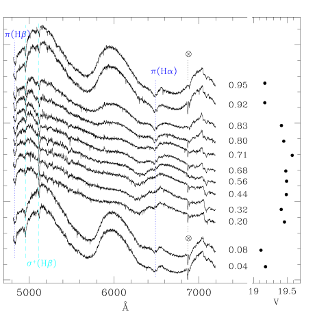
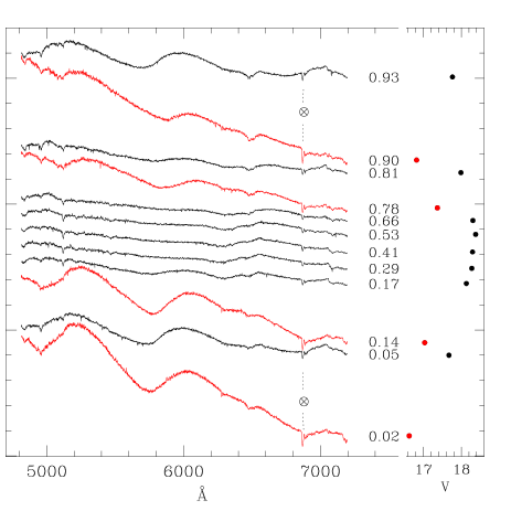
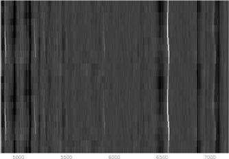
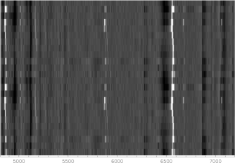
We plot in Figure 1 the two series of spectra after phasing and after having removed the emission lines to enhance the visibility of cyclotron emissions. The second data set probably corresponds to a higher mass transfer rate, being about 1 mag brighter. Clear evidence of a different mass transfer rate is present in the emission lines (intensity, species and profile) which will be analyzed in a separate paper. However, according to the AAVSO records, VV Pup was never brighter than V=16 mag, thus both our data sets sample a low state.

In March 2004, VV Pup was clearly accreting through both magnetic poles as it is evident from the two distinct sets of cyclotron emission/humps which are visible at different orbital phases. During the bright orbital phase ($\sim$0.8-0.2) the spectra are dominated by cyclotron emission peaking at 5170 Å, 6000 Å, and 7050 Å. These cyclotron harmonics are attributed to the main $\sim 32$ MG pole. During the faint orbital phase ($\sim$0.2-0.8), these harmonics disappear and give way to another series of cyclotron peaks at 5000 Å and 6600 Å. This second set forms in the proximity of the stronger ($\sim 56$  MG) magnetic pole. Based on the assumption that the secondary pole is visible at all phases (see, for example, Piirola et al. 1990), we have subtracted the faint phase spectrum from the bright phase spectrum to extract what we expect for the main pole only.

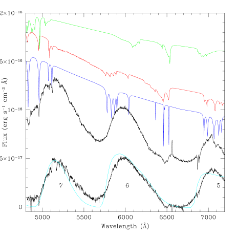
The cyclotron models assume the point source model described in Wickramasinghe and Meggitt (1985). Each model is defined by a set of 4 parameters corresponding to the polar magnetic field, $B_{i}$ (where $i$ is either 1 or 2), the electron temperature, T, the optical depth parameter, $\Lambda$, and the tilting angle, $\delta$, between the field direction and the line of sight. The parameters that best reproduce the main pole spectrum are $B_{1}=31.5$ MG, T=5 Kev, $\log\Lambda=5.5$, $\delta=85^{o}$ for the data taken on the 16th of March and $B_{1}=31.5$ MG, T=7 Kev, $\log\Lambda=5.3$, $\delta=85^{o}$ for those taken on the 22nd of March (see Figure 2, cyan lines). We note that the cyclotron spectrum shows little flux between harmonics $n=5$ and $n=6$ during March 16, consistent with the lower electron temperature of this model. We emphasize that the values of $T$ and $\Lambda$ derived from point source models are indicative of average values over an extended shock region and cannot be directly converted to fluxes without consideration of geometrical effects.

Figure 3: The faint phase spectra (black lines) taken at VLT+FORS1 on the 16th (bottom) and 22nd (top) of March 2004 together with the cyclotron model (cyan line). Also shown are possible contributions from a halo with $B_{h2}=56$ MG (blue line) due to the second magnetic pole and from the photosphere (green and red lines). The photospheric models have $B_{d}=40MG,d=0.11,\theta=45^{\circ}$ (green line) and $B_{d}=60MG,d=0.0,\theta=35^{\circ}$ (red line). See text for more details. The faint spectrum of March 16 is the average of the two spectra at orbital phase 0.44 and 0.56. The faint spectrum of March 22 is the average of the two spectra at orbital phase 0.53 and 0.66. Flux units correspond to the observed spectra, while, the models are in arbitrarily scaled units.

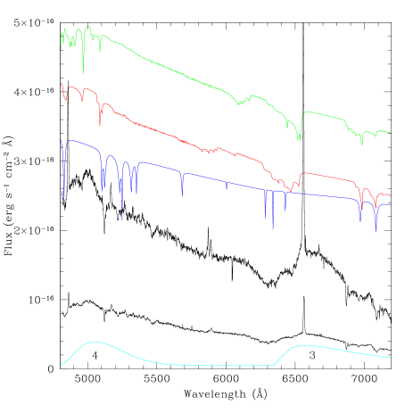
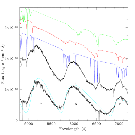
The photosphere is expected to make important contributions during the faint phase, thus it is harder to isolate the properties of the cyclotron component from the faint phase emission. The position of the harmonics, however, allows us to estimate the magnetic field at the second pole with good accuracy, even though the viewing geometry of this region is not well established because it is not eclipsed. The expected positions and relative strengths of the cyclotron lines for a model with $B_{2}=54.6$ MG, T=5 Kev, $\log\Lambda=3.0$, $\delta=75^{\circ}$ are shown in Figure 3. The lower value of this field compared to what was deduced in the discovery spectrum of the second pole (Wickramasinghe et al. 1989) is significant and must indicate a change in the accretion geometry.

Figure 4: Trailed spectrograms of the two VLT data sets. On the right panel the data set taken on 16 March 2004; on the left panel the set taken on 22 March 2004. Spectra are phase ordered from bottom to top and the orbital cycle has been repeated for clarity. However, the phase spacing between two consecutive spectra is not a constant value. Note that the spectra showing stronger H$\alpha$ and H$\beta$ emission as well as the blend HeI(11)$\lambda$5876+NaI$\lambda$5890,5896, correspond to a second orbital cycle, of March 22 observations, which was considerably brighter than the first orbital cycle.

3.2 Zeeman spectra

Narrow absorption features which can be identified as Zeeman components of $H\alpha$ and $H\beta$ are clearly seen in both sets of the March data (Figure 1). Such features are seen in many other AM Herculis type systems and are usually interpreted either as being of photospheric origin or as evidence for absorption in localized regions associated with an accretion shock (an accretion halo).

It is clear from Figure 1 that the absorption features are seen at all phases at nearly the same wavelength. We identify, in particular, the features shortward of $5200$ Å  with $H\beta$ Zeeman components and the structured feature near $6490$ Å with the $\pi$ component of $H\alpha$. The trailed spectra reported in Figure 4 shows that absorption line profiles vary considerably across the orbit. The line profiles change from narrow and sharp during the bright phase to shallow and weak during the faint phase and this prevents the detection of any clear orbital/sinusoidal motion. Line shifts due to changes in the field structure are not expected to be correlated with radial velocity. Their visibility at all phases would suggest that the dominant contribution is from the photosphere. However, the $\sim 56$  MG pole is seen at all phases, and may contribute narrow halo lines, and the $\sim 32$  MG pole may contribute narrow halo lines during the bright phase.

In order to assess whether those absorption lines originate in the photosphere or the halo, we proceed by comparing our spectra with Zeeman absorption as predicted by halo and photosphere models.

There are no detailed theoretical models of the thermal and density structure of accretion halos. An indication of the type of spectra that may be expected from a halo can be obtained by considering the spectra from photospheric patches in a nearly uniform field on the stellar surface in the hypothesis that the halo lines are formed in an effective reversing layer associated with cool gas in the vicinity of the shock. We present the results of such calculations for polar caps with $B_{h1}=32$ MG, $B_{h2}=56$ MG with a field spread of $10$ percent in Figure 2 and 3, respectively (blue lines). Of course, the relative strengths of the $H\alpha$ and $H\beta$ transitions may be quite different from predictions of these models (see Achilleos and Wickramasinghe 1989) depending on the ionization and excitation conditions in the halo. A general observation that applies to all the VLT spectra including the two shown in Figure 2 and 3 is that the widths of the dominant $\pi$ components of $H\alpha$ appear to be much broader than predicted by the halo models. Also, the narrow H$\alpha$ $\sigma^{-}$ component that we expect at $5700$ Å from a $56$ MG halo, is not present in the faint phase data (see Figure 3). These two arguments alone disfavor the halo interpretation of the Zeeman lines.

Conversely, the narrowness of the H$\beta$ absorption features (see in particular the bright phase spectra of Figure 2 and the absorption lines at 4840, 4960 and 5118 Å), seems to support a halo interpretation, if one assumes that the appropriate ionization and excitation conditions prevail in this region. However, it is unlikely that these are halo features from the main $32$ MG pole because the features associated with the blend of the five $\sigma^{-}$ components due to $H\alpha$ near $5800$  Å is not present in our data. Since halo lines are formed against a cyclotron component, these lines should be clearly seen in the data.

We next consider a photospheric interpretation for the Zeeman lines. Off centered dipole models are often used for modeling the underlying field structures in white dwarfs. We consider such models as a first approximation to the field structure. The models are characterized by the dipolar field strength $B_{d}$, the dipole offset $d$ along the dipole axis, the tilt of the dipole axis $\delta_{d}$, and the orbital inclination $i$ (see e.g. Wickramasinghe and Martin 1979).

We present two sets of dipole models. The first set is based on the hypothesis that the cyclotron field determinations can be used to constrain field structure. Previous studies of photometric and polarimetric variations of VV Pup have constrained the location of the cyclotron emission regions on the stellar surface and the orbital inclination $i$. If one makes the assumption that the accretion shocks are located close to the magnetic poles at the foot points of a closed field line, and the field structure is dipolar, the different field strengths measured from the cyclotron lines would indicate a dipole of strength $B_{d}=40$ MG with an offset $d\sim 0.11$ along the dipole axis. Indeed, such a model gives polar field strengths of $57$ MG and $29$ MG. This model requires a tilt of the magnetic dipole axis of $\delta_{d}\sim 30^{\circ}$ to the rotation axis and an orbital inclinations $i\sim 75^{\circ}$ in order to be consistent with the eclipse and polarization constraints (Meggitt and Wickramasinghe 1989). As the dipole rotates, the angle between the line of sight and the dipole axis varies between $\theta=105^{\circ}$, at the center of the bright phase, and $\theta=45^{\circ}$, at the center of the faint phase. The expected faint and bright phase spectra from such a model are shown in Figure 2 and 3 (green lines). These models are clearly also not consistent with the faint or bright phase observations. The central, and strongest $H\alpha$ $\pi$ component is shifted redward from the observed position, and the blend of $H\alpha$ $\sigma^{-}$ components predicted near $6100$ Å is not present in the observations. This is particularly evident at the viewing angle of $\theta=105^{\circ}$ when the more uniform field region containing the weaker pole is in view. The obvious implication is that the two key assumptions involved in these models (namely the closed field line and dipolar field approximation), when taken together, yield inconsistent results. Previous investigators have noted phase shifts between the relative positions of the accretion shocks at different states of activity and have used cyclotron spectroscopy also to argue against the closed field line assumption (e.g. Schwope and Beuermann 1997).

A second alternative approach consists in admitting that the field structures cannot be constrained by cyclotron field determinations (they only provide measurements of the field in two localized regions on the white dwarf surface), and the manner in which the mass transfer stream couples to field lines is essentially unknown. The field structure could then be constrained by analyzing the phase dependence of the absorption lines in conjunction with spectropolarimetric data (e.g. Beuermann et al. 2007). However, such studies are usually best carried out using data obtained when the system is in a truly low state.

We conclude this section by noting that the data currently at hand can nevertheless be used to provide some very general constraints on the underlying field structure. If we restrict our investigations to the class of centered dipole models, and investigate the spectrum at different angles, $\theta$, to the white dwarf rotation axis, we can conclude that there is not a unique centered dipole model capable of explaining all the observations. However, we can find reasonable fits to the data at the center of the bright phase and the center of the faint phase by allowing different values of $B_{d}$. This demonstrates that a field structure that is more complex than a centered dipole is required to model VV Pup spectra. These models are compared with the observations in Figures 2 ($B_{d}=65$ MG and $\theta=55^{\circ}$) and 3 ($B_{d}=60$ MG, $\theta=35^{\circ}$), respectively.

4 Summary and conclusions

We have presented two time series of spectra taken during a low state of the polar VV Pup. Each time series cover about 1 orbital period with a phase resolution of 0.1 per spectrum. The spectra are characterized by very few emission lines (signature of low mass transfer rate), cyclotron emission and Zeeman absorption lines.

In order to identify the exact nature of the Zeeman absorptions we made use of simple models representative of halo or photospheric Zeeman absorptions. In the first case we have shown that the predicted absorptions are more than the observed ones and/or have widths which are inconsistent with observations. On the other side, also the photospheric dipole model predicts a Zeeman spectrum which is in serious disagreement with the observations. In particular, they predict redder absorption lines than observed (off center dipole) or spectral changes with the rotational phase that we do not observe (centered dipole). We conclude that the actual VV Pup field is likely a complex non-dipolar one. We note that multi-pole fields are not uncommon among both isolated magnetic white dwarfs and polars. In particular, complex field structures have been modeled for polars such as EF Eri, BL Hyi and MR Ser (Reincsh et al. 2005), through spectropolarimetry. A better understanding of the underlying field distribution must await detailed spectropolarimetric observations when VV Puppis descends into a truly low state and the bare photosphere is revealed.

Our observations provided clear evidence for accretion onto both magnetic poles. By modeling the cyclotron emissions we find magnetic fields of $31.5$ MG and $54.6$ MG for the main and secondary accretion region, respectively. We note that two pole accretion during a very low state has not been reported before. In the past VV Pup has been observed to accrete through both the magnetic poles (e.g. Visvanathan and Wickramasinghe 1981, Wickramasinghe et al. 1989, Schwope and Beuermann 1997), as well as just the main one (e.g. Wickramasinghe and Visvanathan 1980, Canalle and Opher 1988, Wickramasinghe et al. 1984), during high states.

Polars are known to exhibit different observational characteristics depending on the state of activity of the system. The different states are usually associated with evidence of accretion onto one or two poles, or a combination of the two (see Wickramasinghe and Ferrario 2000, for a review). However, in the case of VV Pup, it seems that there is no correlation between the accretion configuration and the state/ongoing mass transfer rate. This fact questions the mechanism controlling the accretion geometry. There could well be other factors, independent on the mass transfer rate (e.g. star-spots and or active regions on the secondary star, see Howell et al 2006b), which are capable of triggering the two pole accretion. Alternatively, VV Pup could have undergone a change in the relative orientation of the magnetic axis. The latter possibility has already been reported for DQ Leo (Wickramasinghe and Ferrario 2000), for example. However, particularly to prove or disprove the hypothesis of secular variations of the magnetic axis orientation, long term spectropolarimetric observations are needed and encouraged.