Interacting dark energy: generic cosmological evolution for two scalar fields

Abstract

We study the cosmological evolution of two coupled scalar fields with an arbitrary interaction term $V_{T}(\phi,\varphi)$ in the presence of a barotropic fluid, which can be matter or radiation. The force between the barotropic fluid and the scalar fields is only gravitational. We show that the dynamics is completely determine by only three parameters $\lambda_{i},\,i=1,2,3$. We determine all critical points and study their stability. We find six different attractor solutions depending on the values of $\lambda_{i}$ and we calculate the relevant cosmological parameters. We discuss the possibility of having one of the scalar fields as of dark energy while the other could be a scalar field redshifting as matter.

I Introduction

A dark energy component is probably responsible for the present stage of acceleration of our universeDE ,SN . Perhaps the most appealing candidate for dark energy is that of a scalar field, quintessence Q , which can be either a fundamental particle or a composite particle Qax . Within the context of field theory and particle physics it is appealing to interpret the dark energy as some kind of particles that interact with the particles of the standard model very weakly ax.rp . The weakness of the interaction is required since dark energy particles have not been produced in the accelerator and because the dark energy has not decayed into lighter (e.g. massless) fields such as the photon. It is common to assume the interaction between the dark energy and all other particles to be via gravity only, however recently interacting dark energy models have been proposed IDE -wapp . This has been motivated in part by the cosmological observations where an equation of state of dark energy may be smaller than minus DE ,SN . In general fluids with $w<-1$ give many theoretically problems such as stability issues or wrong kinetic terms as phantom fields ph.etc . However interacting dark energy IDE -wapp ,fate , where the dark energy interacts not only gravitationally with other fluids, is a very simple and attractive option which may lead an apparent equation of state smaller than -1 wapp . These fluids can be dark matter, neutrinos or other scalar fields.

We study in this letter the cosmological evolution of the two scalar fields with arbitrary potentials in the presence of a barotropic fluid, which can be matter or radiation. We show that all models dependence lies on three parameters $\lambda_{i},i=1,2,3$ defined in eq.(27). We determine the dynamical equations and obtain the attractor solutions as a function of these $\lambda_{i}$. We find six different attractor solutions depending on the relative size of $\lambda_{i}$ and we calculate the relevant cosmological parameters.

This letter is organized as follows. In section II we set up the framework for the cosmological evolution of two scalar fields with an arbitrary potential in the presence of a barotropic fluid. In section III we present the conditions on the scalar potential for dark energy. In section IV we derive the dynamical first order differential equations and we show that the system is determined by only three parameters. In section V we calculate the critical points and we study the stability of each solution and we give a few examples. In section VI we study different asymptotic limits and we present a discussion on specific particle physics motivated examples. Finally in section VII we present our conclusions.

II Coupled Scalar Fields

Our starting point is a universe filled with two scalar fields $\phi,\varphi$ and a barotropic energy density $\rho_{b}$, which can be either matter $w_{b}=0$ or radiation $w_{b}=1/3$. We will assume that the scalar fields interact via a potential $V_{T}(\phi,\varphi)$ while there is only gravitational interaction between these fields and the barotropic fluid. This work generalizes that of a single scalar field and a barotropic fluid miogen .

One of this scalar fields, namely $\phi$, may be considered as dark energy (quintessence) but it is not necessary to interpret $\phi$ as dark energy and we will work in a completely general framework. We take the following Lagrangian for the scalar fields $\phi$ and $\varphi$

$$L=\frac{1}{2}\partial_{\mu}\phi\partial^{\mu}\phi+\frac{1}{2}\partial_{\mu}\varphi\partial^{\mu}\varphi-V_{T}(\phi,\varphi)$$ (1)

with the total potential $V_{T}(\phi,\varphi)$. Instead of working with the total potential $V_{T}$ we find it useful to separate the contribution of the interacting and non interacting terms to differentiate the contribution of the two scalar fields. So, without loss of generality, we take the total potential as

$$V_{T}(\phi,\varphi)=V(\phi)+B(\phi,\varphi)$$ (2)

with $V(\phi)$ a potential only depending on $\phi$ and the interacting potential $B(\phi,\varphi)$ is a function of both fields. Of course we could take $B(\phi,\varphi)=h(\phi,\varphi)+K(\varphi)$ with $V_{T}=V(\phi)+h(\phi,\varphi)+K(\varphi)$ to have a more symmetric potential between the fields $\phi$ and $\varphi$. However, it is more convenient to keep only the two potentials $V$ and $B$.

The equation of motion of $\phi$ and $\varphi$ for a spatially flat Friedman–Robertson–Walker (FRW) universe are

$$\ddot{\phi}+3H\dot{\phi} = -V_{T\phi}=-V_{\phi}-B_{\phi}$$ (3)

$$\ddot{\varphi}+3H\dot{\varphi} = -V_{T\varphi}=-B_{\varphi}$$ (4)

where the subindex in $V$ and $B$ is defined as $V_{\phi}\equiv\partial V/\partial\phi,B_{\phi}\equiv\partial B/\partial\phi$ and $B_{\varphi}\equiv\partial B/\partial\varphi$. The Hubble parameter $H\equiv\dot{a}/a$ is

$$3H^{2}=\rho=\rho_{\phi}+\rho_{\varphi}+\rho_{b}$$ (5)

where we have taken $8\pi G\equiv 1$ and $\rho$ is the total energy density, $\rho_{b}$ the barotropic fluid and $\rho_{\phi},\rho_{\varphi}$ are defined in eqs.(8) and (9). The mass of the scalar fields is given by

$$m^{2} \equiv \frac{\partial^{2}V_{T}}{\partial\phi^{2}}=V_{\phi\phi}+B_{\phi\phi}$$ (6)

$$M^{2} \equiv \frac{\partial^{2}V_{T}}{\partial\varphi^{2}}=B_{\varphi\varphi}.$$ (7)

We can also define the energy density and pressure for the fields $\phi$ as

$$\rho_{\phi}\equiv\frac{1}{2}\dot{\phi}^{2}+V(\phi),\hskip 14.22636ptp_{\phi}\equiv\frac{1}{2}\dot{\phi}^{2}-V(\phi)$$ (8)

and that of $\varphi$ as

$$\rho_{\varphi}\equiv\frac{1}{2}\dot{\varphi}^{2}+B(\phi,\varphi),\hskip 14.22636ptp_{\varphi}\equiv\frac{1}{2}\dot{\varphi}^{2}-B(\phi,\varphi).$$ (9)

Using eqs.(8) and (9) we can rewrite the dynamical eqs.(3), (4) in terms of the energy densities as

$$\dot{\rho}_{\phi}+3H\rho_{\phi}(1+w_{\phi}) = -\delta=-B_{\phi}\,\dot{\phi}$$

$$\dot{\rho}_{\varphi}+3H\rho_{\varphi}(1+w_{\varphi}) = \delta=B_{\phi}\,\dot{\phi}$$ (10)

$$\dot{\rho}_{b}+3H\rho_{b}(1+w_{b}) = 0$$

where we have included the evolution of the barotropic fluid $\rho_{b}$ and

$$\delta\equiv B_{\phi}\,\dot{\phi}$$ (11)

defines the interaction term. The equation of state parameters are given by

$$w_{\phi}\equiv\frac{p_{\phi}}{\rho_{\phi}}=\frac{\frac{1}{2}\dot{\phi}^{2}-V}{\frac{1}{2}\dot{\phi}^{2}+V},\hskip 28.45274ptw_{\varphi}\equiv\frac{p_{\varphi}}{\rho_{\varphi}}=\frac{\frac{1}{2}\dot{\varphi}^{2}-B}{\frac{1}{2}\dot{\varphi}^{2}+B}$$ (12)

and the time derivative of $H$ is

$$\dot{H}=-\frac{1}{2}\left(\rho_{\phi}+\rho_{\varphi}+\rho_{b}+p_{\phi}+p_{\varphi}+p_{b}\right)=-\frac{1}{2}\left(\dot{\phi}^{2}+\dot{\varphi}^{2}+\rho_{b}(1+w_{b})\right).$$ (13)

II.1 Effective Equation of State

To obtain an effective equation of state we simply rewrite eqs.(II) as

$$\dot{\rho}_{\phi}=-3H\rho_{\phi}(1+w_{eff}),\hskip 28.45274pt\dot{\rho}_{b}=-3H\rho_{b}(1+w_{beff})$$ (14)

with the effective equation of state defined by

$$w_{\phi eff}\equiv w_{\phi}+\frac{B_{\phi}\dot{\phi}}{3H\rho_{\phi}},\hskip 14.22636ptw_{\varphi eff}\equiv w_{b}-\frac{B_{\phi}\dot{\phi}}{3H\rho_{\varphi}}.$$ (15)

We see from eqs.(14) that $w_{\phi eff},w_{\varphi eff}$ give the complete evolution of $\rho_{\phi}$ and $\rho_{\varphi}$. For $B_{\phi}\dot{\phi}>0$ we have $w_{eff}>w_{\phi}$ and the fluid $\rho_{\phi}$ will dilute faster then without the interaction term (i.e. $B_{\phi}\dot{\phi}=0$) while $\rho_{\varphi}$ will dilute slower since $w_{\varphi eff}>w_{\varphi}$. Which fluid dominates at late time will depend on which effective equation of state is smaller. The difference in eqs.(15) is miogen

$$\Delta w_{eff}\equiv w_{\varphi eff}-w_{\phi eff}=\Delta w-\Upsilon$$ (16)

with $\Delta w\equiv w_{\varphi}-w_{\phi}$ and $\Upsilon$ defined as

$$\Upsilon=\frac{B_{\phi}\dot{\phi}}{3H}\left(\frac{\rho_{\phi}+\rho_{\varphi}}{\rho_{\phi}\rho_{\varphi}}\right)$$ (17)

while the sum gives

$$\Omega_{\varphi}w_{\varphi eff}+\Omega_{\phi}w_{\phi eff}=\Omega_{\varphi}w_{\varphi}+\Omega_{\phi}w_{\phi}.$$ (18)

Clearly the relevant quantity to determine the relative growth is given by $\Upsilon$ and if $\Upsilon>\Delta w$ we have $\Delta w_{eff}<0$ and $\rho_{\varphi}$ will dominate the universe at late times while for $\Upsilon<\Delta w$ we have $\Delta w_{eff}>0$ and $\rho_{\phi}$ will prevail. In the limit of no interaction $\delta=B_{\phi}\dot{\phi}=0$ we get $\Upsilon=0$ and $\Delta w_{eff}=\Delta w>0$ if $w_{\phi}<w_{\varphi}$ and $\rho_{\phi}$ will dominate at late times. If $\Upsilon=\Delta w$ then $w_{\varphi eff}=w_{\phi eff}$ and the ratio of both fluids $\rho_{\varphi}/\rho_{\phi}$ will approach a constant value. If the universe is dominated by $\rho_{\phi}+\rho_{\varphi}$, i.e. $\Omega_{\phi}+\Omega_{\varphi}=1$, then eq.(18) gives

$$w_{\phi}\leq\;w_{\phi eff}=w_{\varphi}\Omega_{\varphi}+w_{\phi}(1-\Omega_{\varphi})\;\leq w_{\varphi},$$ (19)

i.e. the effective equation of state is constraint between $w_{\phi}$ and $w_{\varphi}$.

II.2 Effective Potential $V_{T}$

The effective potential $V_{T}$ is defined in eq.(2) and we expect the fields $\phi,\varphi$ to evolve to the minimum of the potential, i.e. $V_{T\phi}=V_{\phi}+B_{\phi}\rightarrow 0$ and $V_{T\varphi}=B_{\varphi}\rightarrow 0$. If we want to interpret $V$ as the dark energy potential, no fine tuning of the potential $V$ requires that the minimum is at vanishing potential (i.e. $V=0$) and $V_{\phi}<0$ (see section III), however including the interaction term $B$ we can now have $V_{T\phi}=0$ for a non vanishing total potential $V_{T}$. A minimum of $V_{T}$ can be reached if $B_{\phi}>0$ since $V_{\phi}<0$ by hypothesis. Taking $V_{T\phi}=0$ and the time derivative $\dot{V}_{T\phi}=V_{T\phi\phi}\dot{\phi}+V_{T\phi\varphi}\dot{\varphi}=m^{2}\dot{\phi}+B_{\phi_{\varphi}}\dot{\varphi}=0$, where we used eq.(6), one obtains wapp

$$\dot{\phi}=-\frac{B_{\phi\varphi}\dot{\varphi}}{m^{2}}\propto a^{-3}$$ (20)

with the solution of $\ddot{\phi}+3H\dot{\phi}\approx 0$ giving de.fer

$$\dot{\phi}\propto a^{-3}.$$ (21)

While the derivative of the effective potential $V_{T\phi}$ is negative the field $\phi$ evolves to larger values and even in the limit $V_{T\phi}=0$ we have with $\dot{\phi}>0$ and a positive the interaction term $\delta=B_{\phi}\dot{\phi}$. The mass $m$ given by eq.(6) becomes wapp

$$m^{2}=V_{\phi\phi}+B_{\phi\phi}=B_{\phi\phi}\left(1+\widetilde{\Gamma}\frac{B_{\phi}^{2}}{BB_{\phi\phi}}\frac{B}{V}\right)\simeq B_{\phi\phi}\left(1+\widetilde{\Gamma}\frac{B_{\phi}^{2}}{BB_{\phi\phi}}\frac{\Omega_{\varphi}}{\Omega_{\phi}}\right)$$ (22)

with $\widetilde{\Gamma}\equiv V_{\phi\phi}V/V_{\phi}^{2}$ ($\widetilde{\Gamma}_{m}\gtrsim 1$ if the field $\phi$ is tracking Q ) and we have approximated $\rho_{\phi}\simeq V$ and $\rho_{\varphi}\simeq B$ in then last equality of eq.(22), valid if the kinetic energy is small compared to the potential energy.

III Dark Energy

We may consider the scalar field $\phi$ as the quintessence field, i.e. dark energy. In the absence of any interaction term with $\varphi$, the lagrangian is simply given by $L(\phi)=\frac{1}{2}\;\dot{\phi}^{2}-V(\phi)$ and $V$ would be the potential responsible for present day acceleration. In this case the slow roll constrains

$$|\frac{V_{\phi}}{V}|\ll 1,\hskip 28.45274pt\frac{V_{\phi\phi}}{V}\ll 1$$ (23)

must be satisfied at present time. As a result of the dynamics, the scalar field will evolve to its minimum and if we do not wish to introduce any kind of unnatural constant or fine tuning problem, the minimum of the potential must have zero energy, i.e. $V|_{min}=V_{\phi}|_{min}=0$ at $\phi_{min}$ miogen .

In the absence of a interaction $B$, a finite value $\phi_{min}$ implies that the scalar field $\phi$ oscillates around its vacuum expectation value (v.e.v.). If the scalar field has a non zero mass or if the potential $V$ admits a Taylor expansion around $\phi_{min}$ then, using the H$\hat{o}$pital rule, one has lim${}_{t\rightarrow\infty}|V_{\phi}/V|=\infty$ and the energy density $\rho_{\phi}$ redshifts with $w_{\phi}=(n-2)/(n+2)$, i.e. $w_{\phi}=0,1/3$ for $n=2,4$ miogen . On the other hand, if $\phi_{min}=\infty$ then $\phi$ will not oscillate and $|V_{\phi}/V|$ will approach either zero, a finite constant or infinity. Only in the case $|V_{\phi}/V|$ going to zero or a constant smaller than $\sqrt{2}$ will the universe accelerate at late times miogen .

The absence of an arbitrary dark energy scale requires the slow roll conditions to be satisfied also in the future and therefore $V$ is a runaway potential and tends to zero at $\phi\rightarrow\phi_{min}=\infty$. From eqs.(23) we see that $V_{\phi}$ and $V_{\phi\phi}$ also approach zero at late times and $V_{\phi}$ is therefore negative. Inflation occurs in general for $\phi\geq 1$ with a mass $m\simeq H$.

IV Generic Dynamical Analysis

To determine the attractor solutions of the differential equations given in eqs.(3) and (4) or (II) it is useful to make the following change of variables miogen ,copeland

$$x_{1}\equiv\frac{\dot{\phi}}{\sqrt{6}H},\hskip 28.45274pty_{1}\equiv\frac{1}{H}\sqrt{\frac{V}{3}}$$ (24)

$$x_{2}\equiv\frac{\dot{\varphi}}{\sqrt{6}H},\hskip 28.45274pty_{2}\equiv\frac{1}{H}\sqrt{\frac{B}{3}}$$ (25)

and eqs.(II) and (13) become a set of dynamical differential equations of first order

$$x_{1N} = -\left(3+\frac{H_{N}}{H}\right)x_{1}+\sqrt{3\over 2}\left(\lambda_{1}y_{1}^{2}+\lambda_{3}\,y_{2}^{2}\right)$$

$$x_{2N} = -\left(3+\frac{H_{N}}{H}\right)x_{2}+\sqrt{3\over 2}\;\lambda_{2}\,y_{2}^{2}$$

$$y_{1N} = -\frac{H_{N}}{H}y_{1}-\sqrt{3\over 2}\;\lambda_{1}\,x_{1}\,y_{1}$$ (26)

$$y_{2N} = -\frac{H_{N}}{H}y_{2}-\sqrt{3\over 2}\left(\lambda_{3}\,x_{1}+\lambda_{2}\,x_{2}\right)y_{2}$$

$$\frac{H_{N}}{H} = -{3\over 2}\left(2x_{1}^{2}+2x_{2}^{2}+\Omega_{b}\gamma_{b}\right)$$

where $N$ is the logarithm of the scale factor $a$, $N\equiv ln(a)$, $\gamma_{b}\equiv 1+w_{b}$, $f_{N}\equiv df/dN$ for $f=x_{i},y_{i},H\;(i=1,2)$, $\Omega_{b}=1-x_{1}^{2}-x_{2}^{2}-y_{1}^{2}-y_{2}^{2}$ and

$$\lambda_{1}(N)\equiv-\frac{V_{\phi}}{V},\;\;\;\lambda_{2}(N)\equiv-\frac{B_{\varphi}}{B},\;\;\;\lambda_{3}(N)\equiv-\frac{B_{\phi}}{B}.$$ (27)

Notice that all model dependence in eqs.(IV) is through the three quantities $\lambda_{i}(N),i=1,2,3$ and the constant parameter $\gamma_{b}=1+w_{b}$. The last eq. of (IV) is constraint between $-3\leq H_{N}/H\leq 0$ for all values of $x_{i},y_{i}$ and $\gamma_{b}$, it takes the value $-3$ when the universe is dominated by the kinetic energy $x_{1}^{2}+x_{2}^{2}=1$ while it becomes $H_{N}/H=0$ when the universe is dominate by a constant potential $y_{1}^{2}+y_{2}^{2}=1$. The set of equations given in eqs.(IV) give the evolution of two scalar fields $\phi,\varphi$ with arbitrary potentials in the presence of a barotropic (perfect) fluid with equation of state $w_{b}=1-\gamma_{b}$. As mentioned in section II the choice of dividing the total potential $V_{T}$ into $V_{T}=V(\phi)+B(\phi,\varphi)$ is without loss of generality and it is convenient in order to distinguish the contribution from both scalar fields. If we do not want to consider the contribution from the barotropic fluid we can easily take the limit $\gamma_{b}=0$ in eqs.(IV) since all contribution form $\rho_{b}$ is given in $H_{N}/H$ via the term $\Omega_{b}\gamma_{b}$. For $\Omega_{b}\neq 0$ we will assume a barotropic fluid with $0<\gamma_{b}<2$ and $\gamma_{b}=1$ for matter while $\gamma_{b}=4/3$ for radiation.

We do not assume any equation of state for the scalar fields. This is indeed necessary since one cannot fix the equation of state and the potential independently. For arbitrary potentials the equation of state for the scalar fields $w_{\phi}=p_{\phi}/\rho_{\phi},\,w_{\varphi}=p_{\varphi}/\rho_{\varphi}$ is determined once

$$\Omega_{\phi}=\frac{\rho_{\phi}}{3H^{2}} = x_{1}^{2}+y_{1}^{2},\hskip 28.45274pt\frac{p_{\phi}}{3H^{2}}=x_{1}^{2}-y_{1}^{2}$$ (28)

$$\Omega_{\varphi}=\frac{\rho_{\varphi}}{3H^{2}} = x_{2}^{2}+y_{2}^{2},\hskip 28.45274pt\frac{p_{\varphi}}{3H^{2}}=x_{2}^{2}-y_{2}^{2}$$ (29)

have been obtained. Alternatively we can solve for $x_{i},y_{i}$ using eqs.(IV) and the quantities $w_{\phi}\equiv w_{1}=(x_{1}^{2}-y_{1}^{2})/(x_{1}^{2}+y_{1}^{2})$ and $w_{\varphi}\equiv w_{2}=(x_{2}^{2}-y_{2}^{2})/(x_{2}^{2}+y_{2}^{2})$ are, in general, time or scale dependent. In terms of $x_{i},y_{i}$ the interaction term in eq.(11) becomes

$$\delta=B_{\phi}\dot{\phi}=-\sqrt{6}\,3H^{3}\lambda_{3}x_{1}y_{2}^{2}$$ (30)

giving an effective equation of state parameters defined in eqs.(15) as

$$w_{\phi eff} = w_{\phi}-\sqrt{\frac{2}{3}}\;\frac{\lambda_{3}\,x_{1}y_{2}^{2}}{\Omega_{\phi}}=\frac{x_{1}^{2}-y_{1}^{2}-\sqrt{\frac{2}{3}}\;\lambda_{3}\,x_{1}y_{2}^{2}}{\Omega_{\phi}}$$ (31)

$$w_{\varphi eff} = w_{\varphi}+\sqrt{\frac{2}{3}}\;\frac{\lambda_{3}\,x_{1}y_{2}^{2}}{\Omega_{\varphi}}=\frac{x_{2}^{2}-y_{2}^{2}(1-\sqrt{\frac{2}{3}}\;\lambda_{3}\,x_{1})}{\Omega_{\varphi}}$$ (32)

and the acceleration of the universe is given by

$$\frac{\ddot{a}}{a} = H^{2}+HH_{N}=-\frac{H^{2}}{2}\left(\Omega_{b}(1+3w_{b})+4(x_{1}^{2}+x_{2}^{2})-2(y_{1}^{2}+y_{2}^{2})\right)$$ (33)

$$= -\frac{H^{2}}{2}\left(4-3\Omega_{b}(1-w_{b})-6(y_{1}^{2}+y_{2}^{2})\right)$$

where we have used $\dot{H}=HH_{N}$ and eq.(IV). Clearly acceleration will occur if the universe is dominated by the potential $y_{T}^{2}\equiv(y_{1}^{2}+y_{2}^{2})=V_{T}/3H^{2}=(V+B)/3H^{2}$, i.e. for $y_{T}^{2}>2/3-\Omega_{b}(1-w_{b})/2$.

V Critical Solutions

We find the critical solutions to the dynamical equations (IV) with $x_{1N}=x_{2N}=y_{1N}=y_{2N}=0$ and solve for constant values of $\lambda_{i},i=1,2,3$. The set of solutions are given in tables 1 and 3. In table 1 we give, for completeness, the unstable critical points and in table 2 we show the values of the equation of state parameters for these solutions. More interesting, we give in table 3 the attractor (stable) solutions. Constant $\lambda$ implies that the potential $V$ and $B$ are exponential potentials, e.g. $V\sim e^{-\alpha\phi}$ with $\lambda_{1}=-V_{\phi}/V=\alpha$ constant. However, if the potential is not exponential we do not expect to have constant $\lambda_{i}$ and they will, in general, evolve with time. In this case we can use the attractor solution of table 3 and take the corresponding limit of $\lambda_{i}$, which will be either zero, constant or infinity miogen , to obtain the asymptotic behavior of the solutions.

In order to determine the stability of the critical points we perturb eqs.(IV) around the critical solution $x_{i},y_{i}$ and we keep linear terms only . The set of eqs. can be written in a matrix form, $Z_{N}=MZ$, where $Z=(\delta x_{1},\delta x_{2},\delta y_{1},\delta y_{2})$ and we diagonalize the matrix $M$. The stability of the solution requires the real part of all eigenvalues to be negative. One of the eigenvalues of model U-I is positive with $Ei=3\gamma_{b}/2>0$ for $\gamma_{b}>0$ while all other models in table 1 have at least one eigenvalue of the form $Ei=3(2-g)>0$ for $0<g<2$. Therefore they are all unstable solutions.

The eigenvalues of models in table 3 are given in table 4. We see that depending on the values of $\lambda_{i}$ the eigenvalues can be negative or positive. For any given choice of $\lambda_{i}$ there is only one stable solution. In table 5 we give the constrains on $\lambda^{\prime}s$ form closure $|x_{i}|\leq 1,y_{i}\leq 1$ and stability arguments. We see that we have two main conditions on $\lambda_{i}$. One is the relative size between $\lambda_{1}^{2}$ and $\lambda_{1}\lambda_{3}$ while the second is the relative size between $\lambda_{2}^{2}+\lambda_{3}^{2}$ and $\lambda_{1}\lambda_{3}$. Depending on the relative size of these two conditions the attractor solution will end up either in models S-I,S-II or S-III,S-IV or S-V, S-VI. A further condition on the magnitude of $\lambda_{i}$ and $3\gamma_{b}$ distinguishes between the different models.

In tables 6 and 7 we give the values of the relevant cosmological parameters such $\Omega_{\phi},\Omega_{\varphi},\Omega_{b},y^{2}_{T}=y_{1}^{2}+y_{2}$ and $w_{\phi},w_{\varphi},w_{\phi eff},w_{\varphi eff},g=\sqrt{2/3}\lambda_{3}x_{1}y_{2}^{2}$. As mentioned in section II.1 the effective equation of state gives the correct redhsift of the scalar field when the interaction term is considered. Attractor solutions S-I and S-II are the critical solution of a single scalar field in the presence of a barotropic fluid. In these models the energy density $\rho_{\varphi}$ redshifts faster than $\rho_{\phi}$ and $\rho_{b}$ so $w_{\varphi eff}$ must be larger than $w_{\phi eff}$ or $w_{b}$. We see from table 7 that models S-III to S-VI have both scalar fields with the same redshift, i.e. $w_{\phi eff}=w_{\varphi eff}$. In models S-III and S-V the redshift is equal to that of the barotropic fluid while in model S-IV and S-VI it depends on the value of the different $\lambda_{i}$ with $w_{\phi eff}=w_{\varphi eff}<w_{b}$. A universe dominated by the barotropic fluid is possible in models S-I, S-III and S-V, while models with no barotropic fluid ($\Omega_{b}=0$) are given by S-II, S-IV and S-VI. An accelerating universe requires $y_{T}^{2}$ to be larger than $2/3-\Omega_{b}/2$ and therefore models S-II, S-IV and S-VI are favored. From table 6 and conditions in table 5 we can see that models S-I, S-III and S-V have $y^{2}_{T}<1-\gamma_{b}/2<1/2$ for $\gamma_{b}\geq 1$ and therefore do not lead to an accelerating universe.

The eigenvalues of model S-V are

$$Ei_{V,1/2} = \frac{3(\gamma_{b}-2)}{4}\pm\frac{3}{4}\sqrt{\frac{(2-\gamma_{b})(24\gamma_{b}^{2}[(\lambda_{1}-\lambda_{3})^{2}+\lambda_{2}^{2}]+(2-9\gamma_{b})\lambda_{1}^{2}\lambda_{2}^{2})}{\lambda_{1}^{2}\lambda_{2}^{2}}}$$ (34)

$$Ei_{V,3/4} = \frac{3(\gamma_{b}-2)}{4}\pm\frac{3}{4}\sqrt{\frac{(2-\gamma_{b})(8\gamma_{b}\lambda_{3}[(\lambda_{1}-\lambda_{3})^{2}+\lambda_{2}^{2}]+(2-9\gamma_{b})\lambda_{1}\lambda_{2}^{2})}{\lambda_{1}\lambda_{2}^{2}}}$$

while of model S-VI are

$$Ei_{VI,1} = \frac{\lambda_{1}^{2}\lambda_{2}^{2}-3\gamma_{b}[(\lambda_{1}-\lambda_{3})^{2}+\lambda_{2}^{2}]}{(\lambda_{1}-\lambda_{3})^{2}+\lambda_{2}^{2}}$$

$$Ei_{VI,2} = \frac{\lambda_{1}^{2}\lambda_{2}^{2}-6[(\lambda_{1}-\lambda_{3})^{2}+\lambda_{2}^{2}]}{2[(\lambda_{1}-\lambda_{3})^{2}+\lambda_{2}^{2}]}$$ (35)

$$Ei_{VI,3/4} = \frac{\lambda_{1}^{2}\lambda_{2}^{2}-6[(\lambda_{1}-\lambda_{3})^{2}+\lambda_{2}^{2}]}{4[(\lambda_{1}-\lambda_{3})^{2}+\lambda_{2}^{2}]}\pm\frac{1}{4}\frac{\sqrt{a_{VI}}}{((\lambda_{1}-\lambda_{3})^{2}+\lambda_{2}^{2})}$$

with

$$a_{VI} \equiv 2ABC+2D^{2}-BE-F^{2}$$

$$A \equiv (\lambda_{1}-\lambda_{3})^{2}+\lambda_{2}^{2},\hskip 28.45274ptB\equiv\lambda_{1}^{2}\lambda_{2}^{2}-6A,\hskip 28.45274ptC\equiv 3\gamma_{b}-\lambda_{1}\lambda_{3},$$ (36)

$$D \equiv 3A(2+\gamma_{b})-2\lambda_{1}^{2}\lambda_{2}^{2},\hskip 14.22636ptE\equiv A(2\lambda_{1}\lambda_{2}-6(1+2\gamma_{b}))+3\lambda_{1}^{2}\lambda_{2}^{2},\hskip 14.22636ptF\equiv 6A(1-\gamma_{b})+\lambda_{1}^{2}\lambda_{2}^{2}$$

The effective equation of state are given by

$$(w_{\phi eff}) = w_{\phi}+\frac{g}{\Omega_{\phi}},\hskip 28.45274pt(w_{\varphi eff})=w_{\varphi}-\frac{g}{\Omega_{\varphi}}$$ (37)

with $g$ given in table 7. For model S-VI we have

$$(w_{\phi})_{VI} = \frac{\lambda_{1}^{2}\lambda_{2}^{4}-(6[(\lambda_{1}-\lambda_{3})^{2}+\lambda_{2}^{2}]-\lambda_{1}^{2}\lambda_{2}^{2})(\lambda_{2}^{2}+\lambda_{3}^{2}-\lambda_{1}\lambda_{3})}{\lambda_{1}^{2}\lambda_{2}^{4}+(6[(\lambda_{1}-\lambda_{3})^{2}+\lambda_{2}^{2}]-\lambda_{1}^{2}\lambda_{2}^{2})(\lambda_{2}^{2}+\lambda_{3}^{2}-\lambda_{1}\lambda_{3})}$$

$$(w_{\varphi})_{VI} = \frac{\lambda_{1}\lambda_{2}^{2}(2\lambda_{1}-\lambda_{3})-6[(\lambda_{1}-\lambda_{3})^{2}+\lambda_{2}^{2}]}{(6[(\lambda_{1}-\lambda_{3})^{2}+\lambda_{2}^{2}]-\lambda_{1}\lambda_{2}^{2}\lambda_{3})}.$$ (38)

V.1 Examples

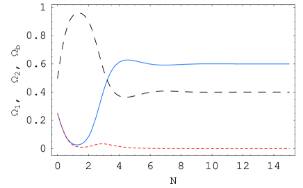
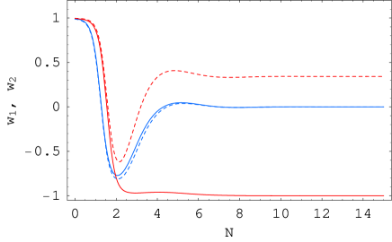
Figure 1: We show the evolution of $\Omega_{\phi}\equiv\Omega_{1},\Omega_{\varphi}\equiv\Omega_{2},\Omega_{b}$ (blue (solid), red (dotted) and black (dashed), respectively) and the equation of state parameters $w_{\phi}=w_{1},w_{\phi eff}$ (blue (solid), blue (dotted)) and $w_{\varphi}=w_{2},w_{\varphi eff}$ (red (solid), red (dotted)) as a function of $N=Log[a]$, for $\lambda_{1}^{2}=5,\lambda_{2}=1,\lambda_{3}=3$ and $\gamma_{b}=1+w_{b}=1$. With these choice of $\lambda^{\prime}s$ the attractor solution is given by model S-I. The attractor solution has $(x_{1},y_{1})=(\sqrt{3/10},\sqrt{3/10})\simeq(0.55,0.55)$ and $(x_{2},y_{2})=(0,0)$.

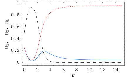
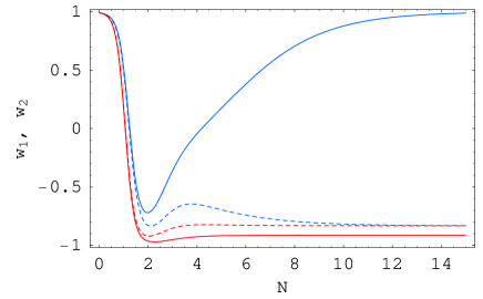
Figure 2: We show the evolution of $\Omega_{\phi}=\Omega_{1},\Omega_{\varphi}=\Omega_{2},\Omega_{b}$ (blue (solid), red (dotted) and black (dashed), respectively) and the equation of state parameters $w_{\phi}=w_{1},w_{\phi eff}$ (blue (solid), blue (dotted)) and $w_{\varphi}=w_{2},w_{\varphi eff}$ (red (solid), red (dotted)) as a function of $N=Log[a]$, for $\lambda_{1}=2,\lambda_{2}=1/2,\lambda_{3}=1/2$ and $\gamma_{b}=1+w_{b}=1$. With these choice of $\lambda^{\prime}s$ the attractor solution is given by model S-IV. The attractor solution has $(x_{1},y_{1})=(0.2,0)$ and $(x_{2},y_{2})=(0.2,0.96)$.

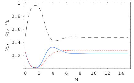
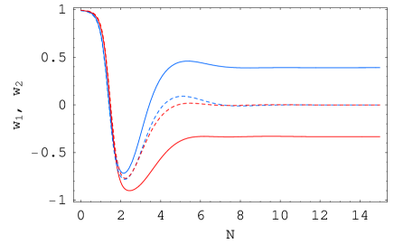
Figure 3: We show the evolution of $\Omega_{\phi}=\Omega_{1},\Omega_{\varphi}=\Omega_{2},\Omega_{b}$ (blue (solid), red (dotted) and black (dashed), respectively) and the equation of state parameters $w_{\phi}=w_{1},w_{\phi eff}$ (blue (solid), blue (dotted)) and $w_{\varphi}=w_{2},w_{\varphi eff}$ (red (solid), red (dotted)) as a function of $N=Log[a]$, for $\lambda_{1}=3,\lambda_{2}=2,\lambda_{3}=3/2$ and $\gamma_{b}=1+w_{b}=1$.With these choice of $\lambda^{\prime}s$ the attractor solution is given by model S-V. The attractor solution has $(x_{1},y_{1})=(0.4,0.3)$ and $(x_{2},y_{2})=(0.3,0.4)$.

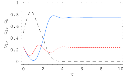
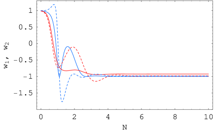
Figure 4: We show the evolution of $\Omega_{\phi}=\Omega_{1},\Omega_{\varphi}=\Omega_{2},\Omega_{b}$ (blue (solid), red (dotted) and black (dashed), respectively) and the equation of state parameters $w_{\phi}=w_{1},w_{\phi eff}$ (blue (solid), blue (dotted)) and $w_{\varphi}=w_{2},w_{\varphi eff}$ (red (solid), red (dotted)) as a function of $N=Log[a]$, for $\lambda_{1}=1,\lambda_{2}=1,\lambda_{3}=-3$ and $\gamma_{b}=1+w_{b}=1$. With these choice of $\lambda^{\prime}s$ the attractor solution is given by model S-VI. The attractor solution has $(x_{1},y_{1})=(0.02,0.87)$ and $(x_{2},y_{2})=(0.1,0.52)$

We now present four different attractor solution depending on the values of $\lambda_{1},\lambda_{2},\lambda_{3}$. We show in figures 1-4 the evolution of $\Omega_{\phi}\equiv\Omega_{1},\Omega_{\varphi}\equiv\Omega_{2},\Omega_{b}$ and $w_{1}\equiv w_{\phi},w_{\phi eff},w_{2}\equiv w_{\varphi},w_{\varphi eff}$ for the different choices of $\lambda^{\prime}s$. We also show the phase space of $(x_{1},y_{1})$ and $(x_{2},y_{2})$ for each case. Since the phase space depends on four variables, namely $(x_{1},y_{1},x_{2},y_{2})$ , it is no surprising that the curves in the two dimensional space $(x_{1},y_{1})$ and $(x_{2},y_{2})$ may cross.

In figs.1 we have $\lambda_{1}^{2}=5,\lambda_{2}=1,\lambda_{3}=3$ and $\gamma_{b}=1+w_{b}=1$ which implies that conditions of model S-I in table 5 are satisfied, i.e. $3=3\gamma_{b}<\lambda_{1}^{2}=5$ and $5=\lambda_{1}^{2}<\lambda_{1}\lambda_{3}\simeq 6.7$. In this case $\rho_{\phi}$ and $\rho_{b}$ have the same redshift at late times and $\Omega_{\phi}/\Omega_{b}$ approaches a constant value while $\rho_{\varphi}$ redshifts faster with an effective $w_{\varphi eff}>w_{b}=0$, even though $w_{2}=w_{\varphi}\rightarrow-1$, and therefore $\Omega_{\varphi}$ tends to zero. The attractor solution has $(x_{1},y_{1})=(\sqrt{3/10},\sqrt{3/10})\simeq(0.55,0.55)$ and $(x_{2},y_{2})=(0,0)$ and $\Omega_{1}=0.6$, $\Omega_{2}=0$ with $\Omega_{b}=0.4$ and $w_{b}=w_{\phi}=w_{\varphi eff}=0$ while $w_{\varphi}=-1$ and $w_{\varphi eff}=0.34$. Since $y_{T}^{2}=y_{2}^{2}+y_{2}^{2}=0.3$ is smaller than $2/3-\Omega_{b}/2=0.87$ then from eq.(33) we conclude that there is no late time acceleration.

In figs.2 we take $\lambda_{1}=2,\lambda_{2}=1/2,\lambda_{3}=1/2$ and $\gamma_{b}=1+w_{b}=1$ which implies that conditions of model S-IV in table 5 are met, i.e. $0.5=\lambda_{2}^{2}+\lambda_{3}^{2}<\lambda_{1}\lambda_{3}=1$ and $3=3\gamma_{b}>\lambda_{2}^{2}+\lambda_{3}^{2}=0.5$. In this case $\rho_{\phi}$ and $\rho_{\varphi}$ have the same redshift at late times and $\Omega_{\phi}/\Omega_{\varphi}$ approaches a constant value while $\Omega_{b}$ goes to zero. The effective equation of state $w_{\phi eff}$ and $w_{\varphi eff}$ have the same late time value $w_{\phi eff}=w_{\varphi eff}\simeq-0.83$ while $w_{\phi}=1$ and $w_{\varphi}=-0.91$. The attractor solution has $(x_{1},y_{1})=(0.2,0)$ and $(x_{2},y_{2})=(0.2,0.96)$ and $\Omega_{1}=0.04$, $\Omega_{2}=0.96$ and $\Omega_{b}=0$. In this case $y_{T}^{2}=y_{2}^{2}+y_{2}^{2}=0.92$ is larger than $2/3-\Omega_{b}/2=2/3$ and from eq.(33) we conclude that the universe accelerates at late times.

In figs.3 we have $\lambda_{1}=3,\lambda_{2}=2,\lambda_{3}=3/2$ and $\gamma_{b}=1+w_{b}=1$ which implies that conditions of model S-V in table 5 are satisfied, i.e. $6.25=\lambda_{2}^{2}+\lambda_{3}^{2}>\lambda_{1}\lambda_{3}=4.5$, $9=\lambda_{1}^{2}>\lambda_{1}\lambda_{3}=4.5$, $18.75=3\gamma_{b}[(\lambda_{1}-\lambda_{3})^{2}+\lambda_{2}^{2}]<\lambda_{1}^{2}\lambda_{2}^{2}=36$ and $9=\lambda_{1}^{2}>3\gamma_{b}^{2}/2=3/2$. In this case $\rho_{\phi},\rho_{\varphi}$ and $\rho_{b}$ have all the same redshift at late times and $\Omega_{\phi},\Omega_{\varphi},\Omega_{b}$ approach a constant value. The effective equation of state $w_{\phi eff}$ and $w_{\varphi eff}$ have the same late time value $w_{\phi eff}=w_{\varphi eff}=w_{b}\simeq 0$ while $w_{\phi}=0.4$ and $w_{\varphi}=-1/3$. The attractor solution has $(x_{1},y_{1})=(0.4,0.27)$ and $(x_{2},y_{2})=(0.3,0.43)$ and $\Omega_{1}=\Omega_{\phi}=0.24$, $\Omega_{2}=\Omega_{\varphi}=0.29$ and $\Omega_{b}=0.47$. Since $y_{T}^{2}=y_{2}^{2}+y_{2}^{2}=0.26$ is smaller than $2/3-\Omega_{b}/2\simeq 0.43$ then from eq.(33) we conclude that the universe does not accelerate at late times.

Finally, in figs.4 we take $\lambda_{1}=1,\lambda_{2}=1,\lambda_{3}=-3$ and $\gamma_{b}=1+w_{b}=1$ which implies that conditions of model S-VI in table 5 are satisfied, i.e. $10=\lambda_{2}^{2}+\lambda_{3}^{2}>\lambda_{1}\lambda_{3}=-3$, $1=\lambda_{1}^{2}>\lambda_{1}\lambda_{3}=-3$, $51=3\gamma_{b}[(\lambda_{1}-\lambda_{3})^{2}+\lambda_{2}^{2}]>\lambda_{1}^{2}\lambda_{2}^{2}=1$ and $17\sqrt{6}=\sqrt{6}|\lambda_{1}|[(\lambda_{1}-\lambda_{3})^{2}+\lambda_{2}^{2}]>\lambda_{1}^{2}\lambda_{2}^{2}=1$. In this case $\rho_{\phi}$ and $\rho_{\varphi}$ have the same redshift at late times and $\Omega_{\phi}/\Omega_{\varphi}$ approaches a constant value while $\Omega_{b}$ goes to zero. The effective equation of state $w_{\phi eff}$ and $w_{\varphi eff}$ have the same late time value $w_{\phi eff}=w_{\varphi eff}\simeq-0.98$ while $w_{\phi}=-0.99$ and $w_{\varphi}=-0.92$. Notice that at some redshifts the effective equation of state take values $w_{\phi eff}<-1$. The attractor solution has $(x_{1},y_{1})=(0.02,0.87)$ and $(x_{2},y_{2})=(0.1,0.48)$ and $\Omega_{1}=\Omega_{\phi}=0.76$, $\Omega_{2}=\Omega_{\varphi}=0.24$ and $\Omega_{b}=0$. Since $y_{T}^{2}=y_{2}^{2}+y_{2}^{2}=0.99$ is smaller than $2/3-\Omega_{b}/2=2/3$ then from eq.(33) we conclude that the universe does accelerate at late times.

Model	$y_{1}$	$y_{2}$	$x_{1}$	$x_{2}$	$\Omega_{1}=\Omega_{\phi}$	$\Omega_{2}=\Omega_{\varphi}$	$\Omega_{b}$
U-I	$0$	$0$	$0$	$0$	$0$	$0$	$1$
U-II	$0$	$0$	$\pm 1$	$0$	$1$	$0$	$0$
U-III	$0$	$0$	$\pm\sqrt{1-x_{2}^{2}}$	$x_{2}$	$1-x_{2}^{2}$	$x_{2}^{2}$	$0$
U-IV	$0$	$0$	$\frac{\sqrt{6}}{\lambda_{1}}$	$\pm\sqrt{1-\frac{6}{\lambda_{1}}}$	$\frac{6}{\lambda_{1}^{2}}$	$1-\frac{6}{\lambda_{1}^{2}}$	$0$
U-V	$0$	$0$	$\frac{\sqrt{6}\lambda_{3}+\lambda_{2}\sqrt{\lambda_{2}^{2}+\lambda_{3}^{2}-6}}{\lambda_{2}^{2}+\lambda_{3}^{2}}$	$\frac{\sqrt{6}\lambda_{2}-\lambda_{3}\sqrt{\lambda_{2}^{2}+\lambda_{3}^{2}-6}}{\lambda_{2}^{2}+\lambda_{3}^{2}}$	$x_{1}^{2}$	$x_{2}^{2}$	$0$
U-VI	$0$	$0$	$\frac{\sqrt{6}\lambda_{3}-\lambda_{2}\sqrt{\lambda_{2}^{2}+\lambda_{3}^{2}-6}}{\lambda_{2}^{2}+\lambda_{3}^{2}}$	$\frac{\sqrt{6}\lambda_{2}+\lambda_{3}\sqrt{\lambda_{2}^{2}+\lambda_{3}^{2}-6}}{\lambda_{2}^{2}+\lambda_{3}^{2}}$	$x_{1}^{2}$	$x_{2}^{2}$	$0$

Table 1: Unstable critical solutions.

Model	$w_{\phi}$	$w_{\varphi}$	$w_{\phi eff}$	$w_{\varphi eff}$	$\Upsilon$
U-I	$-$	$-$	$-$	$-$	$-$
U-II	$1$	$-$	$1$	$-$	$-$
U-III	$1$	$1$	$1$	$1$	$0$
U-IV	$1$	$1$	$1$	$1$	$0$
U-V	$1$	$1$	$1$	$1$	$0$
U-VI	$1$	$1$	$1$	$1$	$0$

Table 2: Equation of state parameters of the unstable solutions of table 1.

Model	$y_{1}$	$y_{2}$	$x_{1}$	$x_{2}$
S-I	$\sqrt{\frac{3(2-\gamma_{b})\gamma_{b}}{2\lambda_{1}^{2}}}$	$0$	$\sqrt{\frac{3}{2}}\frac{\gamma_{b}}{\lambda_{1}}$	0
S-II	$\sqrt{1-\frac{\lambda_{1}^{2}}{6}}$	$0$	$\frac{\lambda_{1}}{\sqrt{6}}$	$0$
S-III	$0$	$\sqrt{\frac{3(2-\gamma_{b})\gamma_{b}}{2(\lambda_{2}^{2}+\lambda_{3}^{2})}}$	$\sqrt{\frac{3}{2}}\frac{\gamma_{b}\lambda_{3}}{\lambda_{2}^{2}+\lambda_{3}^{2}}$	$\sqrt{\frac{3}{2}}\frac{\gamma_{b}\lambda_{2}}{\lambda_{2}^{2}+\lambda_{3}^{2}}$
S-IV	$0$	$\sqrt{1-\frac{\lambda_{2}^{2}+\lambda_{3}^{2}}{6}}$	$\frac{\lambda_{3}}{\sqrt{6}}$	$\frac{\lambda_{2}}{\sqrt{6}}$
S-V	$\sqrt{\frac{3(2-\gamma_{b})\gamma_{b}(\lambda_{2}^{2}+\lambda_{3}^{2}-\lambda_{1}\lambda_{3})}{2\lambda_{1}^{2}\lambda_{2}^{2}}}$	$\sqrt{\frac{3(2-\gamma_{b})\gamma_{b}(\lambda_{1}-\lambda_{3})}{2\lambda_{1}\lambda_{2}^{2}}}$	$\sqrt{\frac{3}{2}}\frac{\gamma_{b}}{\lambda_{1}}$	$\sqrt{\frac{3}{2}}\frac{\gamma_{b}(\lambda_{1}-\lambda_{3})}{\lambda_{1}\lambda_{2}}$
S-VI	$\frac{\sqrt{(6[(\lambda_{1}-\lambda_{3})^{2}+\lambda_{2}^{2}]-\lambda_{1}^{2}\lambda_{2}^{2}))(\lambda_{2}^{2}+\lambda_{3}^{2}-\lambda_{1}\lambda_{3})}}{\sqrt{6}((\lambda_{1}-\lambda_{3})^{2}+\lambda_{2}^{2})}$	$\frac{\sqrt{\lambda_{1}(\lambda_{3}-\lambda_{1})(\lambda_{1}^{2}\lambda_{2}^{2}-6[(\lambda_{1}-\lambda_{3})^{2}+\lambda_{2}^{2}])}}{\sqrt{6}((\lambda_{1}-\lambda_{3})^{2}+\lambda_{2}^{2})}$	$\frac{\lambda_{1}\lambda_{2}^{2}}{\sqrt{6}((\lambda_{1}-\lambda_{3})^{2}+\lambda_{2}^{2})}$	$\frac{\lambda_{1}\lambda_{2}(\lambda_{1}-\lambda_{3})}{\sqrt{6}((\lambda_{1}-\lambda_{3})^{2}+\lambda_{2}^{2})}$

Table 3: Stable critical solutions.

Models	$Ei_{1}$	$Ei_{2}$	$Ei_{3}$	$Ei_{4}$
S-I	$\frac{3}{2}(\gamma_{b}-2)$	$\frac{3}{2}\gamma_{b}(1-\frac{\lambda_{3}}{\lambda_{1}})$	$\frac{3}{4}(\gamma_{b}-2)+\frac{3}{4}\sqrt{\frac{(2-\gamma_{b})(24\gamma_{b}^{2}+(2-9\gamma_{b})\lambda_{1}^{2})}{\lambda_{1}^{2}}}$	$\frac{3}{4}(\gamma_{b}-2)-\frac{3}{4}\sqrt{\frac{(2-\gamma_{b})(24\gamma_{b}^{2}+(2-9\gamma_{b})\lambda_{1}^{2})}{\lambda_{1}^{2}}}$
S-II	$\frac{1}{2}(6-\lambda_{1}^{2})$	$\frac{1}{2}(6-\lambda_{1}^{2})$	$-3\gamma_{b}+\lambda_{1}^{2}$	$\frac{1}{2}\lambda_{1}(\lambda_{1}-\lambda_{3})$
S-III	$\frac{3}{2}(\gamma_{b}-2)$	$\frac{3\gamma_{b}(\lambda_{2}^{2}+\lambda_{3}^{2}-\lambda_{1}\lambda_{3})}{2(\lambda_{2}^{2}+\lambda_{3}^{2})}$	$\frac{3}{4}(\gamma_{b}-2)+\frac{3}{4}\sqrt{\frac{(2-\gamma_{b})(24\gamma_{b}^{2}+(2-9\gamma_{b})(\lambda_{2}^{2}+\lambda_{3}^{2}))}{\lambda_{2}^{2}+\lambda_{3}^{2}}}$	$\frac{3}{4}(\gamma_{b}-2)-\frac{3}{4}\sqrt{\frac{(2-\gamma_{b})(24\gamma_{b}^{2}+(2-9\gamma_{b})(\lambda_{2}^{2}+\lambda_{3}^{2}))}{\lambda_{2}^{2}+\lambda_{3}^{2}}}$
S-IV	$\frac{1}{2}(\lambda_{2}^{2}+\lambda_{3}^{2}-6)$	$\frac{1}{2}(\lambda_{2}^{2}+\lambda_{3}^{2}-6)$	$\lambda_{2}^{2}+\lambda_{3}^{2}-3\gamma_{b}$	$\frac{1}{2}(\lambda_{2}^{2}+\lambda_{3}^{2}-\lambda_{1}\lambda_{3})$
S-V	$Ei_{V,1}$	$Ei_{V,2}$	$Ei_{V,3}$	$Ei_{V,4}$
S-VI	$Ei_{VI,1}$	$Ei_{VI,2}$	$Ei_{VI,3}$	$Ei_{VI,4}$

Table 4: Eigenvalues for the different stable solutions of table 3. Stability requires the real part of all eigenvalues to be negative. Eigenvalues $Ei_{V}$ are given in eqs.(34) while eigenvalues $Ei_{VI}$ in eqs.(V).

Model	$Constraint$	$Constraint$
S-I	$\lambda_{1}^{2}>3\gamma_{b}$	$\lambda_{1}^{2}<\lambda_{1}\lambda_{3}$
S-II	$\lambda_{1}^{2}<3\gamma_{b}$	$\lambda_{1}^{2}<\lambda_{1}\lambda_{3}$
S-III	$\lambda_{2}^{2}+\lambda_{3}^{2}<\lambda_{1}\lambda_{3}$	$\lambda_{2}^{2}+\lambda_{3}^{2}>3\gamma_{b}$
S-IV	$\lambda_{2}^{2}+\lambda_{3}^{2}<\lambda_{1}\lambda_{3}$	$\lambda_{2}^{2}+\lambda_{3}^{2}<3\gamma_{b}$
S-V	$\lambda_{2}^{2}+\lambda_{3}^{2}>\lambda_{1}\lambda_{3}$	$\lambda_{1}^{2}>\lambda_{1}\lambda_{3}$
	$\lambda_{1}^{2}>3\gamma_{b}^{2}/2$	$3\gamma_{b}[(\lambda_{1}-\lambda_{3})^{2}+\lambda_{2}^{2}]<\lambda_{1}^{2}\lambda_{2}^{2}$
S-VI	$\lambda_{2}^{2}+\lambda_{3}^{2}>\lambda_{1}\lambda_{3}$	$\lambda_{1}^{2}>\lambda_{1}\lambda_{3}$
	$\sqrt{6}|\lambda_{1}|[(\lambda_{1}-\lambda_{3})^{2}+\lambda_{2}^{2}]>\lambda_{1}^{2}\lambda_{2}^{2}$	$3\gamma_{b}[(\lambda_{1}-\lambda_{3})^{2}+\lambda_{2}^{2}]>\lambda_{1}^{2}\lambda_{2}^{2}$

Table 5: Constrains on $\lambda_{1},\lambda_{2},\lambda_{3}$ for the different stable solutions of table 3 from closure and stability arguments.

Model	$\Omega_{1}=\Omega_{\phi}$	$\Omega_{2}=\Omega_{\varphi}$	$\Omega_{b}$	$y_{T}^{2}=y_{1}^{2}+y_{2}^{2}$
S-I	$\frac{3\gamma_{b}}{\lambda_{1}^{2}}$	$0$	$1-\frac{3\gamma_{b}}{\lambda_{1}^{2}}$	$\frac{3(2-\gamma_{b})\gamma_{b}}{2\lambda_{1}^{2}}$
S-II	$1$	$0$	$0$	$1-\frac{\lambda_{1}^{2}}{6}$
S-III	$\frac{3\gamma_{b}^{2}\lambda_{3}^{2}}{2(\lambda_{2}^{2}+\lambda_{3}^{2})^{2}}$	$\frac{3\gamma_{b}(2\lambda_{2}^{2}+(2-\gamma_{b})\lambda_{3}^{2})}{2(\lambda_{2}^{2}+\lambda_{3}^{2})^{2}}$	$1-\frac{3\gamma_{b}}{\lambda_{2}^{2}+\lambda_{3}^{2}}$	$\frac{3(2-\gamma_{b})\gamma_{b}}{2(\lambda_{2}^{2}+\lambda_{3}^{2})}$
S-IV	$\frac{\lambda_{3}^{2}}{6}$	1-$\frac{\lambda_{3}^{2}}{6}$	0	$1-\frac{\lambda_{2}^{2}+\lambda_{3}^{2}}{6}$
S-V	$\frac{3\gamma_{b}(2\lambda_{2}^{2}-\lambda_{3}(2-\gamma_{b})(\lambda_{1}-\lambda_{3}))}{2\lambda_{1}^{2}\lambda_{2}^{2}}$	$\frac{3\gamma_{b}(\lambda_{1}-\lambda_{3})(2\lambda_{1}-\gamma_{b}\lambda_{3})}{2\lambda_{1}^{2}\lambda_{2}^{2}}$	$1-\frac{3\gamma_{b}((\lambda_{1}-\lambda_{3})^{2}+\lambda_{2}^{2})}{\lambda_{1}^{2}\lambda_{2}^{2}}$	$\frac{3(2-\gamma_{b})\gamma_{b}[(\lambda_{1}-\lambda_{3})^{2}+\lambda_{2}^{2}]}{2\lambda_{1}^{2}\lambda_{2}^{2}}$
S-VI	$\frac{(6[(\lambda_{1}-\lambda_{3})^{2}+\lambda_{2}^{2}]-\lambda_{1}^{2}\lambda_{2}^{2}))(\lambda_{2}^{2}+\lambda_{3}^{2}-\lambda_{1}\lambda_{3})+\lambda_{1}^{2}\lambda_{2}^{4}}{6[(\lambda_{1}-\lambda_{3})^{2}+\lambda_{2}^{2}]^{2}}$	$\frac{\lambda_{1}(\lambda_{1}-\lambda_{3})(6[(\lambda_{1}-\lambda_{3})^{2}+\lambda_{2}^{2}]-\lambda_{1}\lambda_{2}^{2}\lambda_{3})}{6[(\lambda_{1}-\lambda_{3})^{2}+\lambda_{2}^{2}]}$	$0$	$1-\frac{\lambda_{1}^{2}\lambda_{2}^{2}}{6[(\lambda_{1}-\lambda_{3})^{2}+\lambda_{2}^{2}]}$

Table 6: Energy density for the different stable solutions of table 3.

Model	$w_{\phi}$	$w_{\varphi}$	$w_{\phi eff}$	$w_{\varphi eff}$	$g=\sqrt{\frac{2}{3}}\lambda_{3}x_{1}y_{2}^{2}$
S-I	$w_{b}$	$-$	$w_{b}$	$>w_{b},w_{\phi eff}$	$0$
S-II	$-1+\frac{\lambda_{1}^{2}}{3}$	$-$	$-1+\frac{\lambda_{1}^{2}}{3}$	$>w_{b},w_{\phi eff}$	$0$
S-III	$1$	$-1+\frac{2\gamma_{b}\lambda_{2}^{2}}{2\lambda_{2}^{2}+(2-\gamma_{b})\lambda_{3}^{2}}$	$w_{b}$	$w_{b}$	$\frac{3(2-\gamma_{b})\gamma_{b}^{2}\lambda_{3}^{2}}{2(\lambda_{2}^{2}+\lambda_{3}^{2})}$
S-IV	$1$	$-1+\frac{2\lambda_{2}^{2}}{6-\lambda_{3}^{2}}$	$-1+\frac{\lambda_{2}^{2}+\lambda_{3}^{2}}{3}$	$-1+\frac{\lambda_{2}^{2}+\lambda_{3}^{2}}{3}$	$\frac{\lambda_{3}^{2}(\lambda_{2}^{2}+\lambda_{3}^{2}-6)}{18}$
S-V	$-1+\frac{2\gamma_{b}\lambda_{2}^{2}}{2\lambda_{2}^{2}+(2-\gamma_{b})(\lambda_{3}-\lambda_{1})\lambda_{3}}$	$\frac{2(1-\gamma_{b})\lambda_{1}+\gamma_{b}\lambda_{3}}{\gamma_{b}\lambda_{3}-2\lambda_{1}}$	$w_{b}$	$w_{b}$	$\frac{3(2-\gamma_{b})\gamma_{b}^{2}\lambda_{3}(\lambda_{1}-\lambda_{3})}{2\lambda_{1}^{2}\lambda_{2}^{2}}$
S-VI	$(w_{\phi})_{VI}$	$(w_{\varphi})_{VI}$	$-1+\frac{\lambda_{1}^{2}\lambda_{2}^{2}}{3[(\lambda_{1}-\lambda_{3})^{2}+\lambda_{2}^{2}]}$	$-1+\frac{\lambda_{1}^{2}\lambda_{2}^{2}}{3[(\lambda_{1}-\lambda_{3})^{2}+\lambda_{2}^{2}]}$	$\frac{\lambda_{1}^{2}\lambda_{2}^{2}\lambda_{3}(\lambda_{1}-\lambda_{3})(6[(\lambda_{1}-\lambda_{3})^{2}+\lambda_{2}^{2}]-\lambda_{1}^{2}\lambda_{2}^{2})}{18[(\lambda_{1}-\lambda_{3})^{2}+\lambda_{2}^{2}]^{3}}$

Table 7: Equation of state parameters of the stable solutions of table 3. The equation of state parameters $w_{VI}$ are given in eqs.(V).

VI Asymptotic Behavior

Special cases can be studied by taking different limits of the parameters $\lambda$. From tables 5 and 7 we can determine which values of $\lambda_{i}$ are required for any particular late time behavior we wish to have. For example if we are interested in the behavior of having only two scalar fields and no barotropic fluid ($\Omega_{b}=0$) we can take the limit $\gamma_{b}=0$ of models in table 3. Only models S-II, S-IV and S-VI survive and $x_{i},y_{i}$ take the same values as in table 3. If we prefer a universe dominated by the barotropic fluid than models S-I, S-III and S-V need to be considered. An accelerating universe requires $y_{T}^{2}$ to be larger than $2/3-\Omega_{b}/2$ and therefore models S-II, S-IV and S-VI are favored.

If we take the limit $\lambda_{1}=0$ then only models S-II and S-VI remain consistent and they have $(x_{1},y_{1})=(0,1)$ and $(x_{2},y_{2})=(0,0)$. Models S-I and S-V do not satisfy the closure condition $|x_{i}|\leq 1|,y_{i}\leq 1$) while models S-III and S-IV are no longer stable if $\lambda_{2}\neq 0\neq\lambda_{3}$ (c.f. eigenvalues of table 4). In the limit $\lambda_{1}\rightarrow 0$, the first derivative of the potential approaches zero faster than the potential itself and examples of this kind of behavior are given by potentials of the form $V=V_{0}\phi^{-n},n>0$.

For $\lambda_{2}=0$ only model S-V is no longer consistent. Models S-I and S-II remain the same as in table 3 and model S-III becomes $(x_{1},y_{1})=(\sqrt{3/2}\;\gamma_{b}/\lambda_{3},0)$ and $(x_{2},y_{2})=(0,(\sqrt{3(2-\gamma_{b})\gamma_{b}/2}/\lambda_{3})$, S-IV is now $(x_{1},y_{1})=(\lambda_{3}/\sqrt{6},0)$ and $(x_{2},y_{2})=(0,(\sqrt{1-\lambda_{3}^{2}/6})$ while S-VI becomes $(x_{1},y_{1})=(0,\sqrt{\lambda_{3}/(\lambda_{3}-\lambda_{1})})$ and $(x_{2},y_{2})=(0,\sqrt{\lambda_{1}/(\lambda_{1}-\lambda_{3})})$.

In the case $\lambda_{3}=0$ all models remain valid from closure arguments and are given in table 8. However, models S-I to S-IV are no longer stable for $\lambda_{1}\neq 0\neq\lambda_{2}$, as seen from table 4, and only models S-V and S-VI are the attractor solutions.

Model	$y_{1}$	$y_{2}$	$x_{1}$	$x_{2}$
S-I	$\sqrt{\frac{3(2-\gamma_{b})\gamma_{b})}{2\lambda_{1}^{2}}}$	$0$	$\sqrt{\frac{3}{2}}\frac{\gamma_{b}}{\lambda_{1}}$	$0$
S-II	$\sqrt{1-\frac{\lambda_{1}^{2}}{6}}$	$0$	$\frac{\lambda_{1}}{\sqrt{6}}$	$0$
S-III	$0$	$\sqrt{\frac{3(2-\gamma_{b})\gamma_{b})}{2\lambda_{2}^{2}}}$	$0$	$\sqrt{\frac{3}{2}}\frac{\gamma_{b}}{\lambda_{2}}$
S-IV	$0$	$\sqrt{1-\frac{\lambda_{2}^{2}}{6}}$	$0$	$\frac{\lambda_{2}}{\sqrt{6}}$
S-V	$\sqrt{\frac{3(2-\gamma_{b})\gamma_{b}}{2\lambda_{1}^{2}}}$	$\sqrt{\frac{3(2-\gamma_{b})\gamma_{b}}{2\lambda_{2}^{2}}}$	$\sqrt{\frac{3}{2}}\frac{\gamma_{b}}{\lambda_{1}}$	$\sqrt{\frac{3}{2}}\frac{\gamma_{b}}{\lambda_{2}}$
S-VI	$\frac{\sqrt{\lambda_{2}^{2}[6(\lambda_{2}^{2}+\lambda_{1}^{2})-\lambda_{1}^{2}\lambda_{2}^{2}]}}{\sqrt{6}(\lambda_{1}^{2}+\lambda_{2}^{2})}$	$\frac{\sqrt{\lambda_{1}^{2}(6[(\lambda_{1}^{2}+\lambda_{2}^{2}]-\lambda_{1}^{2}\lambda_{2}^{2})}}{\sqrt{6}(\lambda_{1}^{2}+\lambda_{2}^{2})}$	$\frac{\lambda_{1}\lambda_{2}^{2}}{\sqrt{6}(\lambda_{1}^{2}+\lambda_{2}^{2})}$	$\frac{\lambda_{1}^{2}\lambda_{2}}{\sqrt{6}(\lambda_{1}^{2}+\lambda_{2}^{2})}$

Table 8: Attractor solutions of table 3 in the limit $\lambda_{3}=0$

Finally, if we impose the condition $\lambda_{1}y_{1}^{2}+\lambda_{3}y_{2}^{2}=0$, which minimize the potential as a function of $\phi$, i.e $dV_{T}/d\phi=d(V+B)/d\phi=0$, there are only three attractor solutions to eqs.(IV). The first case is model S-II $(x_{1},y_{1})=(0,1)$ and $(x_{2},y_{2})=(0,0)$ (c.f. table 3 in the limit $\lambda_{1}=-\lambda_{3}y_{2}^{2}/y_{1}^{2}=0$). The other two models are S-III and S-IV of table 3 with the limit $\lambda_{3}=-\lambda_{1}y_{1}^{2}/y_{2}^{2}=0$ (c.f. table 8). There is no stable solution with $\lambda_{i},\,i=1,2,3$ constant and $y_{1}y_{2}\neq 0$. Let us take the limit $\lambda_{1}y_{1}^{2}+\lambda_{3}y_{2}^{2}=0$ in eqs.(IV). The evolution for $x_{1}$ is

$$\frac{x_{1N}}{x_{1}}=-(3+\frac{H_{N}}{H})\leq 0,\hskip 56.9055pt$$ (39)

and since $-3\leq H_{N}/H\leq 0$ for all values of $x_{i},y_{i}$ and $\gamma_{b}$ we conclude that $x_{1}$ will approach its minimum value (i.e. $x_{1}\rightarrow 0$). If $|\lambda_{1}|<\infty$, so that $\lambda_{3}x_{1}\rightarrow 0$, then the evolution of $y_{1}$ becomes

$$\frac{y_{1N}}{y_{1}}=-\frac{H_{N}}{H}-\sqrt{3\over 2}\;\lambda_{1}\,x_{1}\simeq-\frac{H_{N}}{H}\geq 0$$ (40)

and $y_{1}$ will increase to its maximum value (i.e. $y_{1}\rightarrow 1$). Since $x_{1}^{2}+y_{1}^{2}+x_{2}^{2}+y_{2}^{2}+\Omega_{b}=1$ then for $y_{1}=1$ we get $x_{1}=x_{2}=y_{2}=\Omega_{b}=0$ giving model S-II.

VI.1 Particle Physics Model

Let us now take a specific choice of potentials motivated by particle physics. We consider a factorisable interaction potential

$$B(\phi,\varphi)=h(\phi)F(\varphi).$$ (41)

In this case the $\lambda_{i}$ parameters become only functions of a single field

$$\lambda_{1}(\phi)=-\frac{V^{\prime}(\phi)}{V(\phi)},\hskip 8.5359pt\lambda_{2}(\varphi)=-\frac{F^{\prime}(\varphi)}{F(\varphi)},\hskip 8.5359pt\lambda_{3}(\phi)=-\frac{h^{\prime}(\phi)}{h(\phi)}$$ (42)

where the prime denotes derivative w.r.t. its argument. Let us take a simple example where the potential for the scalar field $\phi$ has an exponential behavior, widely used in particle physics as for dark energy potential, while we take a power law potential for $\varphi$ which would represent a standard scalar field. It is well known that for a single scalar field with potential of the form $\varphi^{n}$ the energy density redshifts as $w_{\varphi}=(n-2)/(n+2)$ giving $w_{\varphi}=0,1/3$ for $n=2,4$ miogen . So, we take $V=V_{o}e^{-\alpha\phi},B=B_{o}e^{\beta\phi}\varphi^{n}$ with $V_{o}>0,B_{o}>0$. In this case $\lambda_{1}=\alpha,\lambda_{3}=-\beta,\lambda_{2}=-n/\varphi$ . The effective potential defined in eq.(2) is minimized for

$$V_{T\phi} = V_{\phi}+B_{\phi}=-\alpha V+\beta B=0$$ (43)

$$V_{T\varphi} = B_{\varphi}=nB_{o}e^{-\beta\phi}\varphi^{n-1}=0$$ (44)

which implies $V/h=(V_{o}/B_{o})e^{-(\alpha+\beta)\phi}=(\beta/\alpha)\varphi^{n}$, i.e.

$$\phi=-Log[A\varphi^{n}]/(\alpha+\beta),\hskip 14.22636pth=e^{-[\beta/(\alpha+\beta)]Log[A\varphi^{n}]}=A^{-\beta/(\alpha+\beta)}\varphi^{-n\beta/(\alpha+\beta)}$$ (45)

with $A=B_{o}\beta/V_{o}\alpha$ and $A$ should be positive and we take $\alpha>0,\beta>0$. The condition $h\varphi^{n-1}\rightarrow 0$ becomes

$$h\varphi^{n-1}=h_{o}A^{-\beta/(\alpha+\beta)}\varphi^{[(n-1)\alpha+n\beta]/(\alpha+\beta)}\rightarrow 0$$ (46)

and for $[(n-1)\alpha+n\beta]/(\alpha+\beta)>0$ (valid for $n>1$) we find $\varphi\rightarrow 0$ giving $|\lambda_{2}|\rightarrow\infty$. From table 5 we see that for $|\lambda_{2}|\gg|\lambda_{1}|,|\lambda_{3}|$ the stable solution are given by model S-V or S-VI depending whether $3\gamma_{b}$ is smaller or larger than $\lambda_{1}^{2}=\alpha^{2}$. Model S-V has $(\Omega_{1},\Omega_{2},\Omega_{b},y_{T}^{2})=(3\gamma_{b}/\lambda_{1}^{2},0,1-3\gamma_{b}/\lambda_{1}^{2},3(2-\gamma_{b})\gamma_{b}/2\lambda_{1}^{2})$ and model S-VI has $(\Omega_{1},\Omega_{2},\Omega_{b},y_{T}^{2})=(1,0,0,1-\lambda_{1}^{2}/6)$. We see that in both cases the amount of energy density from the field $\varphi$ vanishes and the solutions reduce to a single scalar field $\phi$ which depending on the value of $\lambda_{1}=\alpha$ we can have a universe completely dominated by the scalar field $\phi$ with an accelerating universe for $\lambda_{1}^{2}<2$ or a scalar field redshifting as the barotropic fluid for $\lambda_{1}^{2}>3\gamma_{b}$. The interaction term $g$ given in table 7 vanishes for models S-V, S-VI in the limit $|\lambda_{2}|\rightarrow\infty$. The equation of state for $\varphi$ for model S-V is $w_{\varphi}=(2(1-\gamma_{b})\lambda_{1}+\gamma_{b}\lambda_{3})/(\gamma_{b}\lambda_{3}-2\lambda_{1})$ while for model S-VI we have $w_{\varphi}=(6+\lambda_{1}\lambda_{3}-2\lambda_{1}^{2})/(\lambda_{1}\lambda_{3}-6)$ (c.f. eq.(V)).

VII Summary and Conclusions

We have studied the dynamical system of two scalar fields with arbitrary potentials in the presence of a barotropic fluid in a FRW metric. We have shown that all model dependence is given in terms of three parameters, namely $\lambda_{1}(N)=-\ V_{\phi}/V,\,\lambda_{2}(N)=-B_{\varphi}/B,\,\lambda_{3}(N)=-B_{\phi}/B$, and we have calculated all critical points and determine their stability. We have seen that there are six different attractor solutions given in table 3. For a given choice of $\lambda_{i}$ the attractor solution depends on the relative magnitude of $\lambda_{1},\lambda_{2},\lambda_{3}$ and $\gamma_{b}$ as discussed in table 5. We have calculated the relevant cosmological parameters and we have shown the phase space for four different attractor solutions. Finally, we have discussed the different asymptotic limits of the parameters $\lambda_{i}$ and we have studied a special type of scalar potential motivated by particle physics.

References

- (1)
- (2) D. N. Spergel et al., astro-ph/0603449; M. Tegmark et al. Phys.Rev.D74:123507,2006; U. Seljak, A. Slosar and P. McDonald,JCAP 0610:014,2006
- (3) A. G. Riess et al. [Supernova Search Team Collaboration], Astrophys. J. 607, 665 (2004); W. M. Wood-Vasey et al., arXiv:astro-ph/0701041; N. Palanque-Delabrouille [SNLS Collaboration], arXiv:astro-ph/0509425.
- (4) I. Zlatev, L. Wang and P.J. Steinhardt, Phys. Rev. Lett.82 (1999) 896; Phys. Rev. D59 (1999)123504
- (5) P. Binetruy, Phys.Rev. D60 (1999) 063502, Int. J.Theor. Phys.39 (2000) 1859; A. de la Macorra, C. Stephan-Otto, Phys.Rev.Lett.87:(2001) 271301; A. De la Macorra JHEP01(2003)033
- (6) A. de la Macorra, Phys.Rev.D72:043508,2005
- (7) A. de la Macorra, G. Piccinelli, Phys.Rev.D61:123503,2000.
- (8) T. Barreiro, Edmund J. Copeland, N.J. Nunes, Phys.Rev.D61:127301,2000.
- (9) L. Amendola, Phys. Rev. D 62, 043511 (2000); M. Kaplinghat and A. Rajaraman, arXiv:astro-ph/0601517. D. B. Kaplan, A. E. Nelson and N. Weiner, Phys. Rev. Lett. 93, 091801 (2004) R. D. Peccei, Phys. Rev. D 71, 023527 (2005) A. W. Brookfield, C. van de Bruck, D. F. Mota and D. Tocchini-Valentini, Phys.Rev.D 73 (2006) 083515; M. Kaplinghat and A. Rajaraman, arXiv:astro-ph/0601517; S. Das, P. S. Corasaniti and J. Khoury,Phys. Rev. D 73, 083509 (2006)
- (10) A. de la Macorra, A. Melchiorri, P. Serra, R. Bean astro-ph/0608351 (to be publsihed in Astrop.Phys.)
- (11) J.Khoury, A.Weltman, Phys.Rev.D69:044026 (2004); P. Brax, C.van de Bruck, A.C.Davis, J.Khoury, A.Weltman Phys.Rev.D70:123518,2004
- (12) S. Das, P. S. Corasaniti and J. Khoury,Phys. Rev. D 73, 083509 (2006)
- (13) A. de la Macorra, astro-ph/0701635.
- (14) S. M. Carroll, M. Hoffman and M. Trodden, Phys. Rev. D 68, 023509 (2003); A. de la Macorra, H. Vucetich, JCAP09(2004)012
- (15) A.de la Macorra, astro-ph/0702239