The time ending the shallow decay
of the X-ray light curves of long GRBs

Abstract

We show that the mean values and distributions of the time ending the shallow decay of the light curve of the X-ray afterglow of long gamma ray bursts (GRBs), the equivalent isotropic energy in the X-ray afterglow up to that time and the equivalent isotropic GRB energy, as well as the correlations between them, are precisely those predicted by the cannonball (CB) model of GRBs. Correlations between prompt and afterglow observables are important in that they test the overall consistency of a GRB model. In the CB model, the prompt and afterglow spectra, the endtime, the complex canonical shape of the X-ray afterglows and the correlations between GRB observables are not surprises, but predictions.

1 Introduction

In a relatively brief time, the observations made or triggered by the Burst Alert Telescope (BAT), the X-Ray Telescope (XRT), and the UVOR telescope, aboard the Swift satellite, have gathered a wealth of new information on Gamma Ray Bursts (GRBs), in particular on the early X-ray and optical afterglows (AGs) of long-duration GRBs. These observations pose severe problems to the generally accepted ‘Fireball’ model of GRBs (see, e.g. Meszaros 2006), whose ‘microphysics’ (see, e.g. Panaitescu et al. 2006), reliance on shocks (see, e.g. Kumar et al. 2007), and correlations based on the ‘jet-opening angle’ (see, e.g. Sato et al. 2007; Burrows & Racusin 2007), may have to be abandoned.

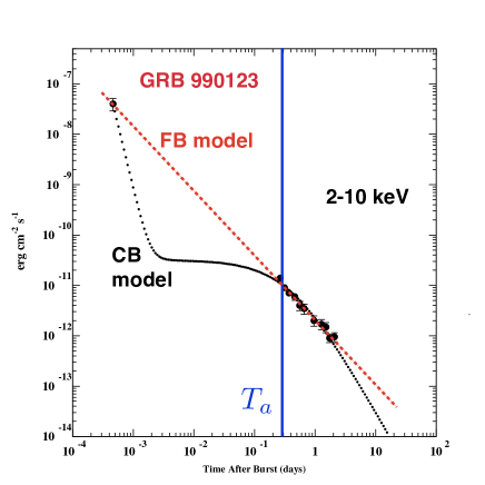
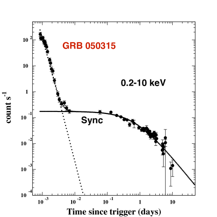
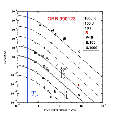
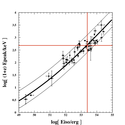
The said recent observations agree remarkably well with the predictions of the ‘Cannon Ball’ (CB) model (Dar & De Rújula 2004; Dado, Dar & De Rújula 2002; Dado, Dar & De Rújula 2003, hereafter DD04; DDD02; DDD03, respectively). Some examples are given in Fig. 1. The predicted lightcurve of the X-ray AG afterglow is shown in Fig. 1a for the fireball (see e.g. Maiorano et al. 2005) and CB (DDD02) models. For GRBs with an approximately constant circumburst density distribution, the well-observed X-ray AGs have a ‘canonical behaviour’ (e.g. Nousek et al. 2006; Zhang et al. 2006; O’brein et al. 2006), in impressive agreement with the CB-model predictions, as in the example of Fig. 1b. The evolution of the AG around the time, $T_{a}$, ending the ‘shallow phase’ is predicted to be achromatic in the optical to X-ray range (DDD02), as can be seen in Fig. 1c and its comparison with Fig. 1d. This ‘achromaticity’ does not extend to the radio domain (DDD03). Many correlations between (prompt) GRB observables have been studied with the help of the new data on GRBs of measured red-shift $z$ (e.g. Schaefer 2006). All of the successful correlations are simple predictions of the CB model. One example, perhaps the best known, is the correlation between the spectral ‘peak’ energy and the total (bolometric) isotropic-equivalent energy, shown in Fig. 1d along with our prediction (Dado at al. 2007 and references therein).

Willinger et al. (2007) have studied and tabulated recent data on $T_{a}$, the time ending the shallow decay of the X-ray light curves of long GRBs. In a paper the title of whose first version was the same as ours, Nava et al. (2007) have investigated the correlation between $T^{\prime}_{a}\equiv T_{a}/(1+z)$, the endtime in the source’s rest frame, and the prompt GRB energy, as well as the correlation between $T^{\prime}_{a}$ and the energy in the X-ray plateau phase, integrated up to $T_{a}$. The values and distributions of these three quantities, as well as their correlations, are important in ascertaining the global validity of a GRB model, among other things because they test the consistency of the description of the prompt and afterglow phases. In this paper we show that the observations are in precise agreement with the CB-model’s predictions. To do so, we gather, in Sections 3, 4 and 5, predictions from various of our papers, in a manner and order adequate to the discussion of the subject at hand. The predictions are derived for ‘typical’ or average values of the parameters, all chosen as in our earlier work, which referred mainly to pre-Swift observations. The incidence and explicit origin of the variability around the typical cases is also discussed. The results are summarized in Fig. 4, which demonstrates that the central expectation, variability and correlations are all as predicted.

2 The CB model

In the CB model (Dar & De Rújula 2000, DD2004; DDD02, DDD03), long-duration GRBs and their AGs are produced by bipolar jets of CBs, ejected in core-collapse SN explosions (Dar & Plaga 1999). An accretion disk is hypothesized to be produced around the newly formed compact object, either by stellar material originally close to the surface of the imploding core and left behind by the explosion-generating outgoing shock, or by more distant stellar matter falling back after its passage (De Rújula 1987). As observed in microquasars, each time part of the disk falls abruptly onto the compact object, a pair of CBs made of ordinary plasma are emitted with high bulk-motion Lorentz factors, $\gamma$, in opposite directions along the rotation axis, wherefrom matter has already fallen onto the compact object, due to lack of rotational support. The $\gamma$-rays of a single pulse in a GRB are produced as a CB coasts through the SN glory –the SN light scattered by the SN and pre-SN ejecta. The electrons enclosed in the CB Compton up-scatter (Shaviv & Dar 1995) glory’s photons to GRB energies.

Each pulse of a GRB corresponds to one CB. The emission times of the individual CBs reflect the chaotic accretion process and are not predictable. At the moment, neither are the characteristic baryon number and Lorentz factor of CBs, which can be inferred from the analysis of GRB afterglows (DDD02; DDD03; DD04). Given this information, two other ‘priors’ (the typical early luminosity of a core-collapse supernova and the typical density distribution of the parent star’s wind-fed circumburst material), and a single extra hypothesis (that the wind’s column density in the ‘polar’ directions is significantly smaller than average) all observed properties of the GRB pulses can be successfully predicted without the introduction of any ad-hoc parameters (Dar & De Rújula 2004, thereafter DD04).

The spectral energy density, $F_{\nu}(t)$, of the X-ray emission of a GRB has two phases. The first is very rapidly declining X-ray emission and dominated by the late-time tail of the GRB pulses (DD04) and/or by line emission and thermal bremsstrahlung from the CBs (DDD02; Dado et al. 2006). In a second phase, synchrotron radiation from swept-in ISM electrons spiraling in the CBs’ enclosed magnetic field takes over. This second phase has a ‘plateau’: a shallow time-dependence lasting until the CBs decelerate significantly in their collisions with the interstellar medium, after which $F_{\nu}(t)$ bends into an asymptotic power-law decline $\sim t^{-1.6}$. On this basis we were able to predict (DDD02) the ‘canonical’ behaviour of X-ray AGs, observed by Swift (Dado et al. 2006).

In the CB model, three times characterize the evolution of $F_{\nu}(t)$. The first is the time at which synchrotron radiation begins to dominate. The second is the time at which the injection bend of the electron energy spectrum within a CB crosses a particular frequency, and corresponds to a strongly chromatic change in $F_{\nu}(t)$ (DDD02; DDD03). The third time, the typical deceleration time, corresponds to an achromatic change in $F_{\nu}(t)$ (DDD02) and is the subject of this paper.

3 The deceleration time

Let $\theta\!=\!{\cal{O}}$(1 mrad) be the typical viewing angle of an observer of a CB that moves with a typical Lorentz factor $\gamma\!=\!{\cal{O}}(10^{3})$. Let $\delta\!=\!{\cal{O}}(10^{3})$ be the corresponding Doppler factor:

$$\delta\equiv{1\over\gamma\,(1-\beta\,\cos\theta)}\simeq{2\,\gamma\over 1+\gamma^{2}\,\theta^{2}}\;,$$ (1)

where the approximation is excellent for $\theta\ll 1$ and $\gamma\gg 1$.

A CB is assumed to contain a tangled magnetic field in equipartition with the ISM protons that enter it. As it ploughs through the ionized ISM, a CB gathers and scatters its constituent protons. The re-emitted protons exert an inward pressure on the CB, countering its expansion. Let $n\simeq n_{p}\simeq n_{e}$ be the number density in a dominantly hydrogenic ISM. In the approximation of isotropic re-emission in the CB’s rest frame and a constant $n$, one finds that within minutes of observer’s time $t$, a CB reaches a nearly-constant ‘coasting’ radius $R$. Subsequently, $\gamma(t)$ obeys:

$$[({\gamma_{0}/\gamma})^{3+\kappa}-1]+(3-\kappa)\,\theta^{2}\,\gamma_{0}^{2}\,[(\gamma_{0}/\gamma)^{1+\kappa}-1]=t/t_{0};\,\,\,\,\,t_{0}\equiv{(1+z)\,N_{b}\over(6+2\kappa)\,c\,n\,\pi\,R^{2}\,\gamma_{0}^{3}}\;,$$ (2)

with $\kappa=1(0)$ depending on whether the re-emitted ISM particles are a small (large) fraction of the intercepted ones. This dichotomy is too small to detect in the study of AGs, but the case $\kappa=1$, which we adopt, is favoured by the CB model of Cosmic Rays (Dar & De Rújula, 2006).

To specify the CB-model’s prediction for an end-time, $T^{\prime}_{a}$, paraphrasing the one defined by Willinger et al. (2007) and Nava et al. (2007), let us derive the time at which the X-ray AG is smaller by a factor of two than the extrapolation from its previous shallow behaviour, and let us refer to the typical parameters of observed GRBs, for which $\gamma_{0}\,\theta\!\sim\!1$, and $\delta(t)\!\approx\!\gamma(t)$ in the shallow phase (DDD02). The X-ray AG, as we shall recall in Section 5, Eq. (12), behaves as $F_{{}_{\rm X}}(t)\!\propto\!\gamma(t)^{6.4}$, so that we are demanding that $[\gamma(t)/\gamma_{0}]^{6.4}\!\simeq\!1/2$. Insert this into the left hand side of Eq. (2), with $\kappa\!=\!1$ and $\theta\gamma_{0}\!=\!1$, to conclude that the typical end-time is $t\!=\!1.026\,t_{0}$. Nava et al. (2007) correct this time for the cosmological redshift; according to Eq. (2), its predicted value is:

$$T^{\prime}_{a} = {T_{a}\over 1+z}\approx 1.026\,{t_{0}\over 1+z}\sim(1.4\times 10^{3}\,{\rm s})\,V_{T}$$

$$V_{T} = \left[{\gamma_{0}\over 10^{3}}\right]^{-3}\,\left[{n\over 10^{-2}\,{\rm cm}^{-3}}\right]^{-1}\,\left[{R\over 10^{14}\,{\rm cm}}\right]^{-2}\,\left[{N_{b}\over 10^{50}}\right],$$ (3)

where we have normalized to typical CB-model parameters and the ‘variability’ around them is governed by the combination of parameters $V_{T}$ (DDD03; Dar & De Rújula 2006).

4 The isotropic energy in the prompt GRB

In the CB model the isotropic (or spherical equivalent) energy, $E_{\gamma}^{\rm iso}$, of a GRB, is (DD04):

$$E_{\gamma}^{\rm iso} \simeq {\delta^{3}\,L_{{}_{\rm SN}}\,N_{{}_{\rm CB}}\,\beta_{s}\over 6\,c}\,\sqrt{\sigma_{{}_{\rm T}}\,N_{b}\over 4\,\pi}\sim(2.8\!\times\!10^{53}\;{\rm erg})\,V_{E},$$

$$V_{E} \equiv {\delta^{3}\over 10^{9}}\,{L_{{}_{\rm SN}}\over L_{{}_{\rm SN}}^{\rm bw}}\,{N_{{}_{\rm CB}}\over 4.5}\,\beta_{s}\sqrt{N_{b}\over 10^{50}}\;,$$ (4)

where $L_{{}_{\rm SN}}$ is the mean SN optical luminosity just prior to the ejection of CBs, $N_{{}_{\rm CB}}$ is the number of CBs in the jet, $N_{b}$ is their mean baryon number, $\beta_{s}$ is the comoving early expansion velocity of a CB (in units of $c/\sqrt{3}$), and $\sigma_{{}_{\rm T}}$ is the Thomson cross section. The early SN luminosity required to produce the mean isotropic energy, $E_{\gamma}^{\rm iso}\!\sim\!4\!\times\!10^{53}$ erg, of ordinary long GRBs is $L_{{}_{\rm SN}}^{\rm bw}\!\simeq\!5\!\times\!10^{42}\,{\rm erg\,s^{-1}}$, the estimated early luminosity of SN1998bw. All quantities in Eq. (4) are normalized to their typical CB-model values. For $N_{{}_{\rm CB}}$ we took the result of a recent careful analysis of the number of significant peaks in a GRB light curve (Schaefer 2006) rather than the one we previously adopted ($N_{{}_{\rm CB}}=6$, DD04).

Nava et al. (2007) choose to present their results in terms of the prompt isotropic energy in the 15-150 keV domain. To restrict the ‘bolometric’ result of Eq. (4) to a fixed-energy bracket, we must recall the prediction of our model for a GRB’s spectral shape (DD04). The photons of the glory’s light that a GRB Compton-upscatters have a thin-bremsstrahlung spectrum $dN/dE_{i}\propto(1/E_{i})^{\alpha}\,{\rm Exp}[-E_{i}/T_{i}]$, with $\alpha\sim 1$ and $T_{i}\sim 1$ eV. The bulk of these electrons are comoving with the CB and Lorentz- and Doppler- boost the target light to a spectrum of the same shape, and ‘temperature’:

$$(1+z)\,T\sim{4\over 3}\;T_{i}\;{\gamma\;\delta}\,\langle 1+\cos\theta_{i}\rangle\sim 1.3\,{\rm MeV}\,\langle 1+\cos\theta_{i}\rangle,$$ (5)

where $\theta_{i}$ is the angle of incidence of a glory’s photon into the CB, in the SN rest system. A very tiny fraction of the moving electrons is due to ‘knock-on’, or is ‘Fermi-accelerated’ within the CB, in both cases to a spectrum (in the CB’s rest frame) $dN_{e}/dE_{e}\propto E^{-p}$, with $p\simeq 2.2$. The complete prompt $\gamma$ spectral distribution, upscattered by the CB’s comoving and knock-on electrons (DD04), is:

$$E\,{dN_{\gamma}\over dE}\propto\left({T\over E}\right)^{\alpha-1}\;e^{-E/T}+b\;(1-e^{-E/T})\;{\left(T\over E\right)}^{p/2}$$ (6)

For $b={\cal{O}}(1)$, and $\alpha$ and $p$ in their expected range, the above spectrum is uncannily similar to the phenomenological ‘Band’ spectrum (Band et al. 1993). The ‘peak energy’ of the prompt spectrum is:

$$(1+z)\,E_{p}\simeq{\gamma\,\delta\,\epsilon_{p}\over 2}\simeq(500\;{\rm keV})\;{\gamma\,\delta\over 10^{6}}\,{\epsilon_{p}\over 1\;\rm eV}\;.$$ (7)

The average redshift of Swift GRBs, and of the ones discussed here, is $\langle z\rangle=2.8$. The fraction $f_{\gamma}$ of the bolometric $E_{\gamma}^{\rm iso}$ lying in the 15-150 keV range is the ratio of $\int\!E\,dN_{\gamma}$ in the range $\langle 1+z\rangle\times$(15-150) keV, to the same integral from 0 to $\infty$: $f_{\gamma}\simeq 0.106$ for all parameters at their central values and $\langle 1+\cos\theta_{i}\rangle=1/2$ (a semitransparent glory, DD04). Our prediction is then:

$$E_{\gamma}^{\rm iso}[15\!-\!150\,{\rm keV}]=f_{\gamma}\,E_{\gamma}^{\rm iso}=(2.9\!\times\!10^{52}\;{\rm erg})\,V_{E},$$ (8)

with $V_{E}$ as in Eq. (4). As the rest of our results, $f_{\gamma}$ is computed for ‘typical parameters’, corresponding to a relatively large $E_{p}$ value and the concomitant large bolometric corrections. For many post-Swift GRBs the bolometric correction would be smaller.

5 The isotropic energy in the X-ray plateau phase

In the plateau phase and thereafter, the CB-model’s AG is due to synchrotron emission by the electrons continuously entering a CB from the interstellar medium (ISM) it sweeps. Above observer’s radio frequencies, and in the CB’s rest system, the synchrotron radiation has a (normalized) spectral shape (DDD03):

$$\nu\,{dn_{\gamma}\over d\,\nu} \propto f_{\rm sync}(\nu,t)={K(p)\over\nu_{b}(t)}{[\nu/\nu_{b}(t)]^{-1/2}\over\sqrt{1+[\nu/\nu_{b}(t)]^{(p-1)}}}$$

$$K(p) \equiv {\sqrt{\pi}\over 2\,\Gamma\left[{2\,p-1\over 2(p-1)}\right]\,\Gamma\left[{p-2\over 2(p-1)}\right]}\approx{p-2\over 2\,(p-1)},$$ (9)

where the ‘injection bend’ frequency $\nu_{b}$ corresponds to the energy, $E_{b}=m_{e}\,c^{2}\,\gamma(t)$, at which ISM electrons enter the CB at the time when its Lorentz factor is $\gamma(t)$. The predicted bend frequency $\nu_{b}$ ($\nu_{b}^{\rm obs}$) in the CB’s (observer’s) frame is:

$${\delta\over 1+z}\,\nu_{b}=\nu_{b}^{\rm obs}\simeq{(5.9\times 10^{15}\;{\rm Hz})\over 1+z}\,{[\gamma(t)]^{3}\,\delta(t)\over 10^{12}}\,\left[{n\over 10^{-2}\;{\rm cm}^{3}}\right]^{1/2}\,.$$ (10)

The typical frequency in the parenthesis is equivalent to an energy of 3.9 eV. This is always below the X-ray domain, so that the corresponding X-ray spectrum has a $\sim\!\nu^{-1.1}$ shape. But, occasionally, at times of order 1 day or less, the observed optical frequencies are above $\nu_{b}^{\rm obs}$, so that the optical spectrum varies from $\sim\!\nu^{-0.5}$ to $\sim\!\nu^{-1.1}$, producing a chromatic break occurring in the optical AG but not in the X-ray one (DDD03).

In a CB’s rest frame, the energy flux density in the optical to X-ray domain is:

$$F_{{}_{\rm CB}}[\nu,t]\simeq\eta\,\pi\,R^{2}\,n\,m_{e}\,c^{3}\,\gamma(t)^{2}\,f_{\rm sync}(\nu,t),$$ (11)

where $\eta$ is the fraction of ISM electrons that enter the CB and radiate there the bulk of their incident energy, and $f_{\rm sync}$ is as in Eq. (9). The AG spectral energy density $F_{\rm obs}$ seen by a cosmological observer at a redshift $z$, is:

$$F_{\rm obs}[\nu,t]\simeq N_{{}_{\rm CB}}\;{(1+z)\,\delta(t)^{3}\over 4\,\pi\,D_{L}^{2}}\,F_{{}_{\rm CB}}\left[{(1+z)\,\nu\over\delta(t)},{\delta(t)\,t\over 1+z}\right]\propto\gamma(t)^{2.3}\,\delta(t)^{4.1}\,,$$ (12)

where $F_{{}_{\rm CB}}$ is as in Eq. (11), and $D_{L}$ is the luminosity distance. As announced in the derivation of Eq. (3), $F_{\rm obs}\propto\gamma^{6.4}$ in the shallow phase of the X-ray afterglow.

With use of the spectrum of Eqs. (9,10) we can define a fraction $f$ of the spectral energy in the 15-150 keV X-ray band. For $p=2.2$:

$$f\equiv K[2.2]\int_{15\,{\rm keV}}^{150\,{\rm keV}}d\nu\;{[\nu_{b}^{\rm obs}]^{0.1}\over\nu^{1.1}}\approx 0.14\,\left[{3.8\over\langle 1+z\rangle}\;{\gamma^{3}\,\delta\over 10^{12}}\;\left({n\over 10^{-2}\,{\rm cm^{-3}}}\right)^{1/2}\right]^{0.1}\;.$$ (13)

Gathering the above results, we obtain for the equivalent isotropic energy per unit observer time in the specified X-ray range:

$$F_{{}_{\rm X}}[15\!-\!150\,{\rm keV}]=f\,F_{{}_{\rm X}}=N_{{}_{\rm CB}}\,\eta\,f\,\pi\,R^{2}\,n\,m_{e}\,c^{3}\,\gamma^{2}\delta^{4}/(1+z)\simeq(9.7\times 10^{47}\,{\rm erg\,s^{-1}})\;\eta\,V_{F}$$

$$V_{F}(t)=\left[{\gamma(t)\over 10^{3}}\right]^{2.3}\,\left[{\delta(t)\over 10^{3}}\right]^{4.1}\,\left[{3.8\over\langle 1+z\rangle}\right]^{1.1}\,\left[{n\over 10^{-2}\,{\rm cm}^{-3}}\right]^{1.05}\,\left[{R\over 10^{14}\,{\rm cm}}\right]^{2}\,\left[{N_{{}_{\rm CB}}\over 4.5}\right]\,,$$ (14)

where we used $\langle 1+z\rangle=3.8$ for the average redshift of GRBs detected by Swift.

The corresponding integrated X-ray energy in the plateau is:

$$I_{{}_{\rm X}}^{\rm iso}\simeq{1\over 2}\,F_{{}_{\rm X}}(t\,=\,0)\,T_{a}=(6.8\times 10^{50}\,{\rm erg})\,V_{T}\,V_{F}(0),$$ (15)

where we took $\eta\simeq 1$, $V_{T}$ and $V_{F}$ are as in Eqs. (3) and (14), and the factor 1/2 reflects the fact that (as can be seen in a plot which is not a logarithmic) most of the plateau, as defined here, extends in the domain where the AG light curve has a value $\sim 1/2$ of its initial value.

6 Results

6.1 Afterglow versus prompt bolometric energies

A simple and crucial test of models of GRBs is the predicted ratio of the bolometric energy in a GRB’s afterglow up to the end of the plateau phase (essentially all of the AG’s energy) and the total energy in the GRB’s prompt $\gamma$ rays. According to Eqs. (14) and (15), the CB-model expectation is:

$$R[{\rm AG/GRB}] = {3\;\delta_{0}\over 4\;\gamma_{0}}\,\sqrt{\pi\,N_{b}\over\sigma_{{}_{\rm T}}}\;m_{e}\,c^{3}\,{\eta\over L_{{}_{\rm SN}}\,\beta_{s}}=0.08\;V_{R}\,,$$

$$V_{R} = {2\over 1+\theta^{2}\,\gamma_{0}^{2}}\;{\eta\over\beta_{s}}\,\sqrt{N_{b}\over 10^{50}}\;{L_{{}_{\rm SN}}^{\rm bw}\over L_{{}_{\rm SN}}}\;.$$ (16)

This ratio is rather ‘clean’: it establishes a link between the late and prompt emissions which is independent of the number of CBs, of their radii, of the density of the ISM in which they travel, and weakly dependent on their baryon number. It very naturally explains why the observed ratios are typically of the order of a few percent.

6.2 Central and typical values

Our main results are Eq. (3) for the time ending the shallow X-ray AG decay, Eq. (8) for $E_{\gamma}^{\rm iso}[15\!-\!150\,{\rm keV}]$, a GRB’s prompt isotropic-equivalent energy in the specified interval, and Eq. (15) for the isotropic energy, $I_{{}_{\rm X}}^{\rm iso}$, in that energy interval of the X-ray AG, integrated in time up to the end of the plateau. The ‘typical’ parameters underlying these results are based on the analysis of pre-Swift GRBs, and reflect the domain wherein GRBs, in the past and with less performing satellites, it was easiest to detect GRBs.

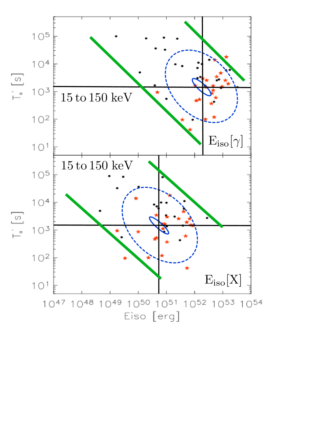
The predicted central expectation for $T^{\prime}_{a}$ is shown in both parts of Fig. 2 as a horizontal line. The central expectations for $E_{\gamma}^{\rm iso}[15\!-\!150\,{\rm keV}]$ and $I_{{}_{\rm X}}^{\rm iso}$ are the vertical lines in the upper and lower part of the figure, respectively. The ‘sweet spot’ drawn as the small ellipses corresponds to letting $\gamma$ and $\delta$ vary in the observed narrow domain wherein most pre-Swift GRBs lied (DDD02; DD04). The larger dotted ellipses are drawn by allowing the combinations of variability parameters, $V$ in Eqs. (3, 8, 15), vary by about an order of magnitude around the small ellipse. As expected, most Swift GRBs with relatively large and measured peak energy (the stars) and relatively large prompt and AG isotropic energies, are within the dotted ellipses. Most of the extra points (the dots) may in the past have been classified as XRFs (they have low ‘peak energy’, $E_{p}$). We discuss them in the next subsection.

The green lines in Fig. 2 show the correlations expected for typical parameters. For them, the $\gamma$ and $\delta$ dependences of the relevant quantities are $T^{\prime}_{a}\propto\gamma_{0}^{-3}$, $E_{\gamma}^{\rm iso}\propto\delta_{0}^{3}$ and $I_{X}^{\rm iso}\propto\gamma_{0}^{-0.7}\,\delta_{0}^{4.1}$, so that $T^{\prime}_{a}\propto 1/E_{\gamma}^{\rm iso}$ and $T^{\prime}_{a}\propto(I_{X}^{\rm iso})^{-3/3.4}$ for $\delta_{0}\approx\gamma_{0}$.

6.3 Distributions and correlations

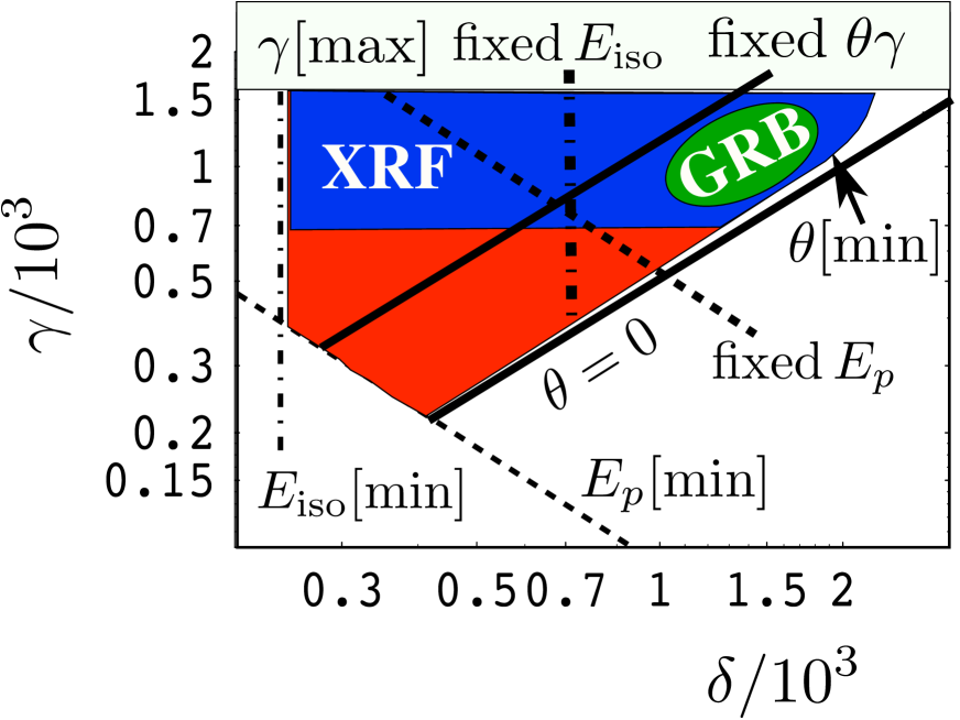
In the CB model, XRFs are the same as GRBs, but observed at a relatively large angle, $\theta$ (or a particularly small $\gamma$), implying a small $\gamma\,\delta$ (DD04; Dado et al. 2004). Thus, XRFs have a relatively small spectral peak energy and a small prompt isotropic energy. The explicit proportionality factors in the relations $E_{p}\propto\gamma\,\delta$ and $E_{\gamma}^{\rm iso}\propto\delta^{3}$ are given by Eqs. (7,4). Consider them fixed at their typical values. The typical $(\gamma,\,\delta)$ domain of observable GRBs is then the one shown in Fig. 3. The observed values of $\gamma$ are fairly narrowly distributed around $\gamma\!\sim\!10^{3}$ (DDD02, DD04), as in the blue strip of the figure. The $(\gamma,\,\delta)$ domain is also limited by a minimum observable isotropic energy or fluence (both $\propto\,\delta^{3}$), by a minimum observable peak energy, and by the line $\theta=0$ or by a line corresponding to a minimum fixed $\theta$, if one takes into account that phase space for observability diminishes as $\theta\to 0$. The elliptical ‘sweet spot’ in Fig. 3 is the region wherein GRBs are most easily detectable, particularly in pre-Swift times. X-ray Flashes populate the region labeled XRF in the figure, above the fixed $\gamma\theta$ line or to the left of the fixed $E_{p}$ line. We interpret most of the dotted points in Figs. 3 and 4 as cases for which $\gamma$ and $\delta$ lie in the ‘XRF domain’ of Fig. 3.

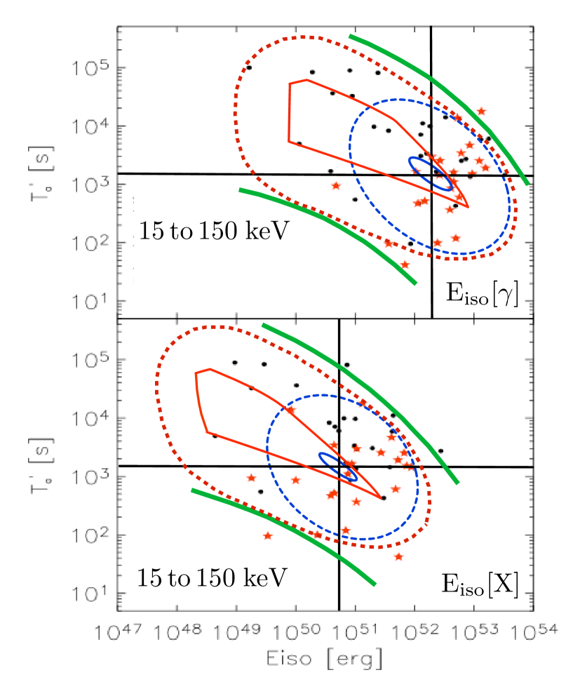
The continuous red lines in Fig. 4 are the contours of the blue domain of Fig. 3, projected into the $[E_{\gamma}^{\rm iso},\,T^{\prime}_{a}]$ plane (top) and the $[E_{X}^{\rm iso},\,T^{\prime}_{a}]$ plane (bottom). The projectors’ are the corresponding functions of $\gamma$ and $\delta$, e.g. $T^{\prime}_{a}(\gamma,\delta)$, as in Eq. (3). The dotted red lines are drawn by ‘moving’ the red contour about its ‘central’ position in the planes, by approximately one order of magnitude, once again to reflect the variability of parameters other than $\gamma$ and $\theta$ (or $\gamma$ and $\delta$). The dotted red lines satisfactorily describe the location and distribution of the Swift data. The green lines are the predicted trend of the correlations, which for the ensemble of the data (stars and points) interpolates between two power laws, as in Fig. 1d, and as discussed in detail for this and many other correlations in Dado et al. 2007.

7 Conclusions

We have analised data on two afterglow observables (the time ending the shallow decay of X-ray AGs and the integrated isotropic energy up to that point) as well as a prompt-GRB observable (the isotropic energy). To do so, we have simply reported the theoretical expectations of the CB model, developed in previous papers. The predictions include the magnitudes of these quantities, the explicit dependence on the parameters that govern their case-by-case variability, and the spectral shapes of the prompt and afterglow phases.

The results can best be summarized by looking at Fig. 4, whose data points are those in the corresponding figure in Nava et al. (2007) who discuss, among others, the same subject. The predictions of the CB model, predating the Swift data, are in excellent agreement with the observations. The data are centered and distributed as expected. Their correlations are also the expected ones, though, since the data points do not span a large number of orders of magnitude, they are not as remarkable as for other correlations, such as the one in Fig. 1a.

In our opinion, the main novelty in the paper of Nava et al. (2007) is the discussion of correlations between prompt-GRB and GRB-afterglow observables. These test the ensemble and coherence of a GRB-model’s ingredients. In the CB model the prompt $\gamma$ rays are of Compton origin, while the AG light is dominated by synchrotron radiation. Unlike fireball models based on very different physics, the CB model never had an ‘energy crisis’ (see e.g. Piran 2000) in the relation between the total energies in the prompt and afterglow phases, or a problem with the prompt spectrum (see, e.g. Ghisellini 2003). The time ending the shallow afterglow phase is a ‘deceleration time’ of the cannon-balls, unrelated to the opening jet-angle of fireball models. The CB model provides very simple, predictive and successful descriptions of the prompt (DD04, Dado et al. 2007) and afterglow phases (DDD02; DD03; Dado et al. 2006; Dado et al., in preparation). We are not surprised that the model is also successful in the detailed description of the distributions of prompt and afterglow observables, and of their correlations.

Acknowledgment: This research was supported in part by the Asher Space Research Fund at the Technion.

Figure 1: Top left: Pre-Swift predictions for the 2-10 keV X-ray AG in the CB (DDD02) and fireball (Maiorano et al. 2005) models, compared to data for GRB 990123. $T_{a}$ is the time ending the plateau phase. Top right: Broad band optical data on GRB 990123, fit in the CB model (DDD03). The evolution is achromatic all the way up to the X-ray energies. Bottom left: Comparison between the CB model prediction and the canonical 0.2-10 keV X-ray light curve of GRB 050315 (Vaughan et al. 2006) Bottom right: The $(E_{p},\,E_{\gamma}^{\rm iso})$ correlation, compared with its predicted trend in the CB model (Dado et al. 2007). The crossed red lines are the predicted typical or average values, see Eqs. (4,7).

Figure 2: The central and typical values, discussed in Section 6.2, for the time ending the X-ray plateau, plotted against the isotropic energies of the prompt $\gamma$ rays and of the X-ray AG up to that time. The data are those gathered by Nava et al. (2007). The crossing lines are the predictions of Eqs. (3,8,15). Within the small ellipse, the parameters $\gamma_{0}$ and $\delta_{0}$ are allowed to range in the small domain in which most pre-Swift GRBs gathered. The larger ellipse allows for the relevant combinations of the other case-by-case parameters to vary by about one order of magnitude. The thick (green) lines are the expected trend of the correlations.

Figure 3: The domain of $(\delta,\,\gamma)$ values. The green elliptical spot labeled ‘GRB’ is the area wherein most pre-Swift GRBs were observed. The region to its left has relatively small (large) $\delta$ ($\theta$) values, corresponds to relatively small $E_{\gamma}^{\rm iso}$ and $E_{p}$, and is labelled ‘XRF’. The blue horizontal band is limited above and below, reflecting the narrow distribution of the $\gamma$ values of observable CBs (DDD02; DD04).

Figure 4: The time ending the X-ray plateau, plotted against the isotropic energies of the prompt $\gamma$ rays and of the X-ray AG up to that time. The data, crossing lines and ellipses are as in Fig. 2. The red line in the top figure is the projection of the contour of the blue $(\gamma,\,\delta)$ domain of Fig. 3 onto the $(T^{\prime}_{a},\,E_{\gamma}^{\rm iso})$ plane. It encompasses the area in which GRBs and XRFs are expected to lie, for all parameters set to their central values, but for $\gamma$ and $\delta$. The red dashed contour is obtained by letting the rest of the relevant combinations of parameters vary by about one order of magnitude. The green thick lines show the expected trend of the correlations. The lower figure is built in the same way, in the $(T^{\prime}_{a},\,E_{X}^{\rm iso})$ plane.

References

- (1) Band, D., Matteson, J., Ford, L., Schaefer, B., Palmer, D., Teegarden, B., Cline, T., Briggs, M., Paciesas, W., Pendleton, G., Fishman, G., Kouveliotou, C., Meegan, C., Wilson, R. and Lestrade, P. et al. ApJ, 413, 281
- (2) Burrows, D. N., Racusin, J., 2007, astro-ph/0702633, to be published in Nuovo Cimento
- (3) Dado, S., Dar, A., De Rújula, A., 2002, A&A, 388, 1079
- (4) Dado, S., Dar, A., De Rújula, A., 2003, A&A, 401, 243
- (5) Dado, S., Dar, A. & De Rújula, A., 2003b, ApJ, 594, L89
- (6) Dado, S., Dar, A. & De Rújula, A., 2004, A&A, 422, 381
- (7) Dado, S., Dar, A., De Rújula, A., 2006, ApJ, 646, L21
- (8) Dado, S., Dar, A., De Rújula, A., 2007, ApJ, 663,
- (9) Dado, S., Dar, A., 2005, Nuovo Cimento 120, 731
- (10) Dar, A., Plaga, R., 1999, A&A, 349, 259
- (11) Dar, A., De Rújula, A., 2000, astro-ph/0008474
- (12) Dar, A., De Rújula, A., 2004, Physics Reports, 405, 203
- (13) Dar, A., De Rújula, A., 2006, hep-ph/0606199
- (14) De Rújula, A., 1987, Phys. Lett. 193, 514
- (15) Ghisellini, G., 2003, astro-ph/0301256, Proc. “Gamma Ray Bursts in the Afterglow Era”. Third Rome workshop. September 2002, Rome
- (16) Kumar, P., McMahon, E., Panaitescu, A., Willingale, R., O’Brien, P., Burrows, D., Cummings, J., Gehrels, N., et al., 2007, MNRAS, 376, L57
- (17) Maiorano, E., Masetti, N., Palazzi, E., Frontera, F., Grandi, P., Pian, E., Amati, L., Nicastro, L., et al., 2005, A&A, 438, 821
- (18) Meszaros, P., 2006, Rept. Prog. Phys. 69 (2006) 2259
- (19) Nava, L., Ghisellini, G., Ghirlanda, G., Cabrera, J. I., Firmani, C., Avila-Reese, V., 2007, astro-ph/0701705, to be published in MNRAS
- (20) Nousek, J. A., Kouveliotou, C., Grupe, D., Page, K. L., Granot, J., Ramirez-Ruiz, E., Patel, S. K., Burrows, D. N., et al., 2006, ApJ, 642, 389
- (21) O’Brien, P. T., Willingale, R., Osborne, J., Goad, M. R., Page, K. L., Vaughan, S., Rol, E., Beardmore, A., et al., 2006, ApJ, 647, 1213
- (22) Panaitescu, A., Mesz ros, P., Burrows, D., Nousek, J., Gehrels, N., O’Brien, P., Willingale, R., 2006, MNRAS, 369, 2059
- (23) Piran, T., 2000, Phys. Rept. 333, 529
- (24) Sato, G., Yamazaki, R., Ioka, K., Sakamoto, T., Takahashi, T., Nakazawa, K.; Nakamura, T., Toma, K., et al., 2007, ApJ 657, 359
- (25) Schaefer, B. E., 2006, astro-ph/0612285
- (26) Shaviv, N. J., Dar, A. 1995, ApJ, 447, 863
- (27) Vaughan, S., Goad, M. R., Beardmore, A. P., O’Brien, P. T., Osborne, J. P., Page, K. L., Barthelmy, S. D., Burrows, D. N., 2006, ApJ, 638, 920
- (28) Willingale, R., O’Brien, P. T., Osborne, J. P., Godet, O., Page, K. L., Goad, M. R., Burrows, D. N., Zhang, B., et al., 2007, astro-ph/0612031
- (29) Zhang, B., 2006, astro-ph/0611774, to be published in Adv. Sp. Res.