Where are the Cosmic Metals at $z\sim 3$ ?

Abstract

The global temperature distribution of the cosmic gas-phase oxygen at $z$$\sim$3 is determined by combining high resolution cosmological simulations of individual proto-galactic, as well as larger, regions with the observed, extinction-corrected, rest-frame V-band galaxy luminosity function. The simulations have been performed with three different stellar initial mass functions (IMFs), a Kroupa (K98), a Salpeter (S) and an Arimoto- Yoshii (AY), spanning a range of a factor of five in chemical yield and specific SNII energy feedback. Gas-phase oxygen is binned according to $T$ as log$(T)\la 4.0$ (“cold”), log$(T)\sim 4.5$ (“warm”), and log$(T)\sim$5.0, 5.5, 6.0, 6.5, 7.0 (“hot” phases). Oxygen is found to be distributed over all $T$ phases, in particular for the top-heavy AY IMF. But, at variance with previous works, it is found that for the K98 and S IMFs the cold phase is the most important. For these IMFs it contains 47 and 37%, respectively, of all gas-phase oxygen, mainly at fairly high density, $n_{\rm{H}}$$\ga$0.1 cm^-3. The implications of this in relation to observational damped Lyman-$\alpha$ absorber (DLA) studies are discussed. In relation to “missing metals” it is found that a significant fraction of the oxygen is located in a warm/hot phase that may be very difficult to detect. Moreover, it is found that less than about 20-25% of the cosmic oxygen is associated with galaxies brighter than $M_{\rm{V}}\sim-22$, i.e., the faintest galaxy luminosities probed by current metallicity determinations for Lyman Break Galaxies (LBGs). Hence, 75-80% of the oxygen is also in this sense “missing”. From the LBG based, $\lambda$$\sim$1500 Å UV luminosity density history at $z$$\geq$3, we obtain an essentially IMF independent constraint on the mean oxygen density at $z$=3. We compare this to what is obtained from our models, for the three different IMFs. We find that the K98 IMF is strongly excluded, as the chemical yield is simply too small, the Salpeter is marginally excluded, and the AY matches the constraint well. The K98 IMF can only match the data if the $\lambda$$\sim$1500 Å extinction corrections have been overestimated by factor of $\sim$4, which seems highly unlikely. The yields for K98 are also far too small to match the observational data for C iv. The optimal IMF should have a yield intermediate between the S and AY.

Where are the Cosmic Metals?

1 Introduction

A number of “problems” have been discussed in relation to the cosmic mean metallicity and/or mean metal density. Pagel (1999) discussed the low redshift ($z$$\sim$0) “excess metals problem” showing that a comparison of the average metal to stellar densities in the low-$z$ Universe indicates that the average cosmic stellar initial mass function (IMF) has a higher yield, than what is obtained for the “standard” Salpeter (1955) IMF. This is a well known result for ellipticals in clusters (e.g., Romeo et al. 2006 and references therein), but Pagel’s analysis indicates that it could be more universal.

Conversely, Pettini (1999) formulated the high-$z$ “missing metals problem” as follows: Studies of the co-moving rest-frame UV luminosity density of high-$z$ Lyman break galaxies (LBGs) allow us to trace the cosmic star formation density (or history, SFH), $\dot{\rho}_{\star}(z)$, up to redshifts $z_{max}\approx 7-8$. Assuming an IMF of such stars, one can compute the specific fraction of heavy elements (“metals”) they produce, $y$, and derive the metal production rate $\dot{\rho}_{Z}(z)=y\dot{\rho}_{\star}(z)$. The integral from $z_{max}$ gives, at any given $z$, the density of cosmic metals $\rho_{Z}^{SFH}(z)$, or, expressed in units of the critical density, $\Omega_{Z}^{SFH}$. Moreover, if one restricts the analysis to elements, such as the $\alpha$-elements, produced almost exclusively in massive stars undergoing core collapse, the apparent dependence of $\rho_{Z}^{SFH}(z)$ on the IMF is essentially removed, since both the UV light and the oxygen production originate from massive stars. This will be discussed further in Section 2, and was already noticed by, e.g., Songaila et al. (1990), Madau et al. (1996), Pagel (1999) and Pettini (1999).

Early searches in cosmic structures for which the metal/baryon mass ratio (metallicity, $Z=\Omega_{Z}/\Omega_{b}$) can be derived either via intergalactic gas quasar absorption line experiments (DLAs or the Ly$\alpha$ “forest”) or through direct spectroscopic studies of Lyman break galaxies have found that only $\Omega_{Z}^{OBS}\la 0.20\Omega_{Z}^{SFH}$ is stored in these components, i.e., the large majority of the metals are “missing”. Similar missing metal problems have been formulated by Wolfe et al. (2003) and Prochaska et al. (2003, 2006) on the basis of star formation rates and metallicities of DLAs alone.

Ferrara et al. (2005, FSB05) attempted to quantify more precisely the extent of the missing metals deficit, and also to suggest where the “missing metals” might be found. They found from considering typical stellar masses and metallicities of Lyman break galaxies, and an estimate of the co-moving density of LBGs a contribution of $\Omega_{Z}^{LBG}=3.4\times 10^{-6}$ from Lyman break galaxies. They also estimated the contribution from metals in DLAs to about $\Omega_{Z}^{DLA}=3.8\times 10^{-7}$. Using the SFH estimate of Bouwens et al. (2004b), assuming a Salpeter IMF, and applying a dust correction factor of 4.5 (Reddy & Steidel 2004) they estimated that the Universe should be characterised by a total metallicity density of $\Omega_{Z}^{SFH}=1.84\pm 0.34\times 10^{-5}$ at $z$=2.3. From the above numbers they concluded that about 80% of the metals in the Universe are missing, in the sense that they are not directly associated with the above two galactic components.

FSB05 suggested that the “missing metals” are associated with galaxies, mainly residing in their “hot” gas halos, having been deposited there by star-burst driven super-winds (see also Pettini 2004). This hypothesis seems reasonable, given that outflow velocities of 300-400 km/s are routinely inferred from the spectra of LBGs (e.g., Pettini et al. 2001, Shapley et al. 2003). Moreover, semi-analytical as well as fully hydrodynamical models of galaxy formation, based on Cold Dark Matter (CDM), require such “feedback” in order to enable the formation of realistic galaxies, solving the “over-cooling”, “angular momentum”, “missing satellites” and other problems (e.g., Sommer-Larsen et al. 1999, Cole et al. 2001, Thacker & Couchman 2001, Sommer-Larsen et al. 2003, SGP03).

Considering the widely used probes of Ly$\alpha$ forest metal absorption in QSO spectra, C iv and O vi (e.g., Songaila 2001, Bergeron et al. 2002, Carswell et al. 2002, Boksenberg, Sargent & Rauch 2003, Schaye et al. 2003, Simcoe et al. 2004, Aracil et al. 2004, Scannapieco et al. 2005; and Bergeron & Herbert-Fort 2005, Tripp et al. 2006), FSB05 inferred observed integrated C iv and O vi column densities over the redshift range 1.7$<$$z$$<$3.8, and the corresponding cosmic average densities of these. Assuming a two-phase intergalactic medium (IGM), consisting of a “cold” part ($T$$\sim$10⁴K), responsible for the hydrogen Ly$\alpha$ forest absorption, and a “hot” component ($T$$\sim$10⁶K), they showed, using a number of simplifying assumptions, that more than 90% of the metals can reside in the hot component, without violating the C iv and O vi Ly$\alpha$ forest metallicity constraints (and with the cold phase as the major contributor to the C iv and O vi column densities). This result follows provided that $T_{hot}\sim$10^5.5K, and the density of the hot metal-enriched gas is only factors of a few times the mean cosmic baryonic density, which, e.g., at $z$=3, corresponds to a hydrogen number density of $n_{\rm{H}}$$\sim$1.2$\times$10^-5cm^-3. FSB05 suggest this metal containing gas to be identified as wind-blown galaxy halo gas.

The low luminosity galaxies at high redshift are traced by the DLAs (e.g. Fynbo et al. 1999; Haehnelt et al. 2000, Schaye 2001a; Møller et al. 2002). From very early on it was found that DLAs contain different regions with very different temperatures and ionisation states (Turnshek et al. 1989). The DLA metal content discussed by FSB05 only accounts for the cold, mainly neutral component. The C iv and Si iv lines in DLAs corresponds to a warmer phase with more turbulent kinematics. The cross-section for strong C iv and Si iv absorption is much larger than for DLAs consistent with the picture that this gas is located in an extended wind-blown halo around the stellar components (Petitjean & Bergeron 1994, see also Adelberger et al. 2003, 2005, Porciani & Madau 2005, Scannapieco 2005). An even hotter component, traced by O vi and N v (temperatures of order $3\times 10^{5}$ K), has recently been identified in DLAs (Fox et al. 2007). Fox et al. find that if the temperature of the O vi bearing gas is 10⁶ K or higher, then this hot phase can contribute significantly to the metal mass budget — qualitatively consistent with the proposal of FSB05.

Bouché et al. (2006a,b) discussed the missing metals problem at $z$$\sim$2.2-2.5 and found that the problem is not quite as severe as at $z$$\sim$3. Counting metal contributions from stars in BX galaxies (the equivalent of LBGs at $z$=2.2; e.g., Adelberger et al. 2004) and DRGs (“distant red galaxies”; e.g., Franx et al. 2003, van Dokkum et al. 2003), as well as from gas in SMGs (sub-millimeter galaxies; e.g., Blain et al. 2004, Greve et al. 2005) and DLAs (e.g., Pettini et al. 2003) they could account for about 1/3 of the metals expected. The BX galaxies contain the largest fraction of the identified metals, about 55%. Moreover, Bouché et al. (2007) found that another about 1/3 of the metals expected can be identified in the IGM at such redshifts.

Recently, Davé & Oppenheimer (2006, DO06) modeled the enrichment history of the Universe and address the missing metals problem using a fully numerical approach. They perform a moderate resolution cosmological hydro/gravity simulation of a cubic region of the Universe of 32 $h^{-1}$Mpc box size. Their simulation invokes metallicity and UV background dependent radiative cooling, star-formation and chemical evolution, in the instantaneous recycling approximation, and based on the Salpeter IMF. The simulation resolves galaxies of stellar masses down to $\sim$10⁹ $M_{\odot}$, corresponding to a V-band absolute magnitude $M_{\rm{V}}$$\sim-20$ at $z$$\sim$3. Due to the limited resolution, the authors adopt a parameterized description of star-burst driven outflows in the form of a “momentum-driven” wind, found by Oppenheimer & Davé (2006, OD06) to yield the best match of the results of their simulations to various observational data.

DO06 quantify their results in terms of cosmic metal fractions in five phases: a) stars, b) star-forming gas, c) halo gas (gas inside of the virial radius of galaxy halos, which is not star-forming), d) shocked IGM (gas outside of galaxy halos of $T$$\geq$3$\times$10⁴ K), and e) diffuse IGM (gas outside of galaxy halos of $T$$<$3$\times$10⁴ K). At $z$$\sim$3, they find that the dominant metal phase is the diffuse IGM, which contains about 40% of the cosmic metals, with the other four phases containing approximately equal fractions of about 15%. Hence, DO06 find that indeed only about 20% of the metals in the $z$$\sim$3 Universe reside in stars, while the “missing” about 80% are located in the gas phase. Moreover, they find that the hot halo gas is not the dominant, metal containing phase. Instead, a large fraction of the missing metals are “hidden” in the diffuse IGM. DO06 suggest that this is possible, in relation to observations of, e.g., low density IGM C iv abundances, because the diffuse gas is somewhat hotter than assumed in previous estimates, which at gas over-densities of $\delta=\rho_{\rm{gas}}/\bar{\rho}_{\rm{gas}}$$\sim 1-100$ implies larger C iv to C ionisation corrections, and hence that larger amounts of C can be “hidden” in this phase.

In this paper we take another approach from that of DO06 (see also Calura & Matteucci 2004, 2006). As we will show in the paper, due to resolution limitations DO06 likely fail to account for about half of the metals in the Universe produced by $z$$\sim$3, on top of which adds cosmic variance effects, given the relatively small computational box of DO06. To undertake simulations of larger cosmological volumes, at the same time probing 8-10 magnitudes deeper (Sec. 5) is at present, as well as in any foreseeable future, computationally prohibitive. Using K-band observations of a sample of LBGs, Shapley et al. (2001) determined the $z$$\sim$3 rest-frame V-band galaxy luminosity function. In Sommer-Larsen & Fynbo (2007, paper I) we correct the Shapley et al. luminosity function for extinction and other effects, to obtain a “true” $z$$\sim$3 Lyman break galaxy LF. Subsequently, cosmological high-resolution hydro/gravity simulations of the formation and evolution of individual galaxies are combined with the corrected galaxy luminosity function to obtain estimates of the average cosmic density of metals (in particular oxygen) residing in stars at $z$=3. We consider models based on three different stellar IMFs, spanning almost a factor of five in chemical yield as well as thermal/kinetic energy feedback from supernova type II (SNII) explosions. These are the Kroupa (1998, K98) IMF, a typical IMF suited for chemical evolution models of the Solar Neighbourhoohd, e.g., Boissier & Prantzos (1999), the “standard” Salpeter (1955, S) IMF and the Arimoto-Yoshii (1987, AY) IMF, which is well suited for describing the chemical evolution of elliptical galaxies. The simulations have sufficiently high resolution to allow a two-phase modeling of the star-forming interstellar medium (ISM), consisting of a “cold” $T$$\sim$10⁴ K star-forming phase and a “hot” $T$$\sim$10⁵- 10⁶ K phase, intermixed with the cold gas. Star-bursts drive galactic winds by depositing thermal energy from multiple SNII explosions in the gas, part of which is subsequently converted into kinetic energy self-consistently by the hydro-code.

In paper I we conclude that for none of the IMFs is it possible to reconcile the amount of oxygen locked in stars with the amount predicted from the (observed) cosmic UV luminosity density history, hence confirming the “missing metals problem” as stated by Pettini (1999) and FSB05.

In this paper we combine the high-resolution galaxy formation models with the V-band luminosity function to determine the cosmologically averaged amount and properties of $z$=3 gas-phase metals, mostly focusing on oxygen, but also on carbon, in particular in relation to QSO absorption line determinations of the cosmic C iv density, as well as iron, in relation to DLA abundances. Combining the results obtained with those of paper I the total cosmic metal distribution is obtained for the three IMFs considered. Comparing in turn these results to inferences from the observed cosmic UV luminosity density history allows us to significantly constrain the “true” cosmic stellar IMF. Finally, relations to the “missing metals problem”, as well as results obtained by other authors, are discussed.

The paper is organised as follows: In section 2 we derive constraints on cosmic metal production from the cosmic UV luminosity density history, in section 3 we briefly describe the hydro/gravity galaxy formation simulations, and in sections 4 and 5 we present the approach used in this paper to determine the temperature distribution of the cosmic gas-phase metals. Section 6 presents results on gas-phase C iv abundances, and, relating these to observations of C iv absorption lines in QSO spectra, we derive a constraint on the cosmic IMF. In section 7 we combine the results of paper I and those obtained here to derive the total cosmic metal distribution. Comparing this to what is obtained from the cosmic UV luminosity density history we obtain an additional constraint on the cosmic stellar IMF. In section 8 we relate our results to the “missing metals problem” and compare them to those of other workers in the field, in section 9 we demonstrate that our results are robust to changes of the numerical resolution and, finally, section 10 summarises our conclusions.

In the paper we assume the flat $\Lambda$ cosmology, with $\Omega_{M}$ = 0.3 and $\Omega_{\Lambda}$=0.7, and $H_{0}=100h$ km/s/Mpc, with $h$=0.7, unless it is explicitly stated otherwise.

2 Constraints on metal production from the cosmic UV luminosity density history

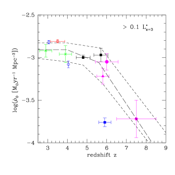
Figure 1: Cosmic oxygen enrichment history based on observations of high-$z$ Lyman break galaxies. The data points shown are based on Steidel et al. (1999; green crosses), Schiminovich et al. (2005; open red dot), Sawicki & Thompson (2006; open blue dots), Giavalisco et al. (2004; black squares), Bunker et al. (2004; blue square), Bouwens et al. (2004a; magenta triangle), Bouwens et al. (2006; magenta circle), Bouwens et al. (2004b; magenta pentagon — note that the latter only represents $L\geq$0.3$\times L^{*}_{UV,z=3}$). The “maximum” model is shown by the upper short-dashed curve, the “median” model by the long-dashed, and the “minimum” model by the lower short-dashed.

Constraints on metal production from the cosmic UV luminosity density history are discussed in paper I, but for coherence we present the main discussion in the following as well.

The luminosity of young galaxies at rest-frame $\lambda\sim$1500 Å is a measure of the rate of formation of massive stars (mainly O and B type) as shown by, e.g., Madau et al. (1998). Moreover, $\alpha$-elements like oxygen are almost exclusively produced in such massive stars, and hence there is a direct link between the cosmic average oxygen production rate density and the average UV luminosity density, which is essentially independent of the stellar initial mass function — see, e.g., Pettini (1999). To estimate the cosmic oxygen production rate density as a function of redshift we use various recent estimates of the average cosmic star formation rate. The estimates have been obtained from Steidel et al. (1999), Bouwens et al. (2004a,b), Bunker et al. (2004), Giavalisco et al. (2004), Schimonovich et al. (2005), Bouwens et al. (2006) and Sawicki & Thompson (2006). The estimates used are all based on assuming a “standard” Salpeter IMF in converting from UV luminosity to star formation rate. The oxygen (mass) yield of a Salpeter IMF is 0.01 (e.g., Lia et al. 2002a,b) — hence in Fig. 1 we have multiplied the published SFRs by 0.01 to obtain the (essentially) IMF independent oxygen production rate densities. The estimates have moreover been corrected to correspond to (at any redshift) the UV luminosity density of galaxies brighter than 0.1$\times L^{*}_{UV,z=3}$ following an approach similar to that of Bouwens et al. (2006; note though that the $z$$\sim$7.5 data point of Bouwens et al. 2004b only represents $L\geq$0.3$\times L^{*}_{UV,z=3}$). Finally, the values shown in the plot result from multiplying the observed values by a dust-correction factor of 5.5. This value is intermediate between the $z\sim$3 values of 4.5 and 6.5 suggested by Reddy & Steidel (2004) and Dahlen et al. (2007), respectively (but see below).

The cosmic average oxygen density at $z$=3 can now be obtained by integrating the oxygen production rate density, $\dot{\rho}_{O}(z)$, from $z$=3 and back in time. We shall consider three models for $\dot{\rho}_{O}(z)$: the “median” model, the “maximum” model, and the “minimum” model. The median model is obtained by calculating the median values of $\dot{\rho}_{O}$ in the bins $z$=3 to 4 and $z$= 4 to 6 (assigning equal weight to each data point, but excluding the $z$=5.9 value of Bunker et al. 2004; see below), and connecting these values with the $z\simeq$7.5 value of Bouwens et al. (2004b). This model is shown in Fig. 1 by the long-dashed curve. The maximum model is obtained by connecting the $z$=3 to 4 median value with the Giavalisco et al. (2004) $z\simeq$5.7 value, and the Bouwens et al. (2004b) $z\simeq$6.0 value, and multiplying the resulting “upper envelope” by a factor 6.5/5.5 to maximize also the dust correction. This model is shown by the upper short-dashed curve in Fig. 1. Finally, the minimum model is obtained by connecting the $z$=3 to 4 median value with the Giavalisco et al. (2004) $z\simeq$4.8 value, the Bouwens et al. (2004a) value and the Bouwens et al. (2006) $z\simeq$7.5 value, and multiplying this “lower envelope” by a factor 4.5/5.5 to minimize the dust correction (but see below). This model is shown by the lower short-dashed curve in Fig. 1.

Assuming a flat space world model, the $z$=3 cosmic average oxygen density can now be evaluated as

$$\rho_{O}(z\mathrm{=3})=-\int_{t(z=3)}^{0}\dot{\rho}_{O}(z(t))~{}dt~{}~{}=$$

$$\frac{1}{H_{0}}\int_{3}^{\infty}\frac{\dot{\rho}_{O}(z)}{(1+z)\sqrt{(1+z)^{2}(1+z\Omega_{M})-z(2+z)\Omega_{\Lambda}}}~{}dz,$$ (1)

where values of $H_{0}=100h$ km/s/Mpc, with $h$=0.7, $\Omega_{M}$ = 0.3 and $\Omega_{\Lambda}$=0.7 are assumed in this paper. Using eq. 1 we obtain $\rho_{O}(z$=3) = 0.32, 0.42 and 0.56 $\times 10^{7}$ $M_{\odot}$/($h^{-1}$Mpc)³ for the “minimum”, “medium” and “maximum” models, respectively. These numbers represent an integral constraint that any successful model of galaxy formation must meet. As will be shown in section 5 this enables us to strongly constrain the “cosmic” stellar IMF at $z\geq$3.

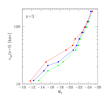
Figure 2: Relation between virial radius and absolute V-band (rest-frame) magnitude at $z$=3 for the K98 (green), Salpeter (blue) and AY (red) IMFs.

In determining the “median” and “minimum” models we excluded the $z$=5.9 value of Bunker et al. (2004). This is simply done on the basis of the large discrepancy between this value, and all other $z$=4 to 6 values. To indicate the effect of this, we determined an alternative median model in which the Bunker et al. (2004) value is included in the $z$=4 to 6 bin. This changed the median model estimate of $\rho_{O}(z$=3) from 0.42 to 0.40 $\times 10^{7}$ $M_{\odot}$/($h^{-1}$Mpc)³, i.e. a $\sim$2 % change, and hence quite small effect, which, given all other uncertainties, we shall ignore in the following.

Bouwens et al. (2006) propose that the $\lambda\sim$1350-1500 Å extinction correction decreases with increasing $z$ from $z\sim$3. Converting their proposed, extinction-corrected SFR($z$) to a corresponding $\dot{\rho}_{O}(z)$ (including changing the UV luminosity density from their limit of 0.04$\times L^{*}_{UV,z=3}$ to the limit of 0.1$\times L^{*}_{UV,z=3}$ used here) results in a value of $\rho_{O}(z$=3) = 0.33 $\times 10^{7}$ $M_{\odot}$/($h^{-1}$Mpc)³, hence within the bounds derived above.

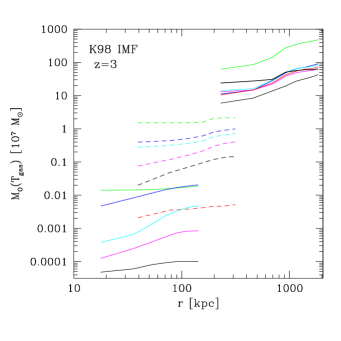
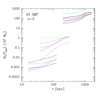
Figure 3: Cumulative mass of gas-phase oxygen with galacto-centric distance for the same three galaxies at $z$=3, simulated with the K98 IMF (left) and the AY IMF (right). Gas temperature colour coding is as follows: $\log(T)$=4: green, 4.5: blue, 5: cyan, 5.5: magenta, 6: black, 6.5: red, 7 black (thick line). For all galaxies the region from $r_{vir}$ to 8 $r_{vir}$ is shown. For the K98 IMF, the galaxies have V-band absolute magnitudes of $-16.1$, $-21.4$ and $-25.3$. For the AY IMF, the corresponding numbers are $-13.8$, $-19.3$ and $-25.4$. The corresponding stellar masses are 5.8$\times 10^{7}$ $M_{\odot}$, 7.3$\times 10^{9}$ $M_{\odot}$ and 3.4$\times 10^{11}$ $M_{\odot}$ for the K98, and 6.4$\times 10^{6}$ $M_{\odot}$, 5.2$\times 10^{8}$ $M_{\odot}$ and 2.5$\times 10^{11}$ $M_{\odot}$ for the AY IMF.

The integral constraint obtained in this section can also be expressed in units of the critical density: we obtain $\Omega_{O}$($z$=3) = $\rho_{O}(z$=3)/$\rho_{\rm{crit}}$ = 0.81, 1.05 and 1.41$\times 10^{-5}$ for the minimum, median and maximum models, respectively.

FSB05 obtained for the total density of heavy elements in units of the critical $\Omega_{Z}$ = (1.84$\pm$0.34)$\times 10^{-5}$, by integrating the observed cosmic star formation history (SFH, based on a Salpeter IMF), as presented by Bouwens et al. (2004b), to $z$=2.3 and applying a dust correction factor of 4.5. The above value translates into $\Omega_{O}$($z$=2.3) = (0.77$\pm$0.14)$\times 10^{-5}$. If the oxygen density production rate models shown in Fig. 1 are continued $z$=2.3, we would obtain 1.22, 1.55 and 2.01 $\times 10^{-5}$. The reason for the apparent discrepancy is two-fold: a) we use a dust correction of a factor of 5.5, and b) more importantly, the Bouwens et al. (2004b) SFH was based on a UV luminosity to a limit of 0.3$\times L^{*}_{UV,z=3}$, rather than the limit of 0.1$\times L^{*}_{UV,z=3}$ adopted in this work. Using the $z\sim 3$ UV luminosity function of Adelberger & Steidel (2000) we estimate the latter correction to be a factor of 1.5. Multiplying this by a factor of 5.5/4.5 the findings of FSB05 would translate into about (1.4$\pm$0.3)$\times 10^{-5}$, in good agreement with our values above.

Extremely dust-obscured galaxies such as high-$z$ SCUBA sources (e.g., Smail et al. 1997; Barger et al. 1998; Eales et al. 1999; Chapman et al. 2005) are not included in the dust-corrected star formation rate densities shown in Fig. 1. Most such galaxies have UV luminosities that heavily under-represent their star formation rates and thus such galaxies are not properly included in the estimate of the oxygen production rate density. Their numbers may be sufficiently large that their contribution is significant, however we neglect this contribution for two reasons: a) the contribution from such galaxies would be largest at $z$$\sim$2, where the redshift distribution of SCUBA sources appears to peak (Chapman et al. 2005, Reddy et al. 2005), whereas we are concerned with the range $z$$\ga$3, and b) more importantly, we are concerned with the oxygen production rate density history of Lyman Break Galaxies only, as we wish to compare the integral constraint thus obtained to results of combining the observed LBG $z$$\sim$3 optical rest-frame luminosity function with detailed, high-resolution models of galaxy formation.

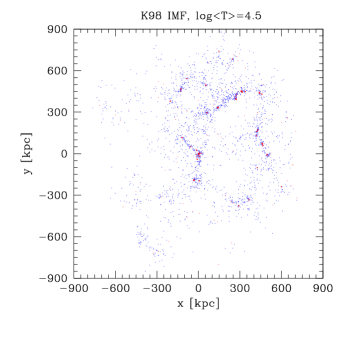
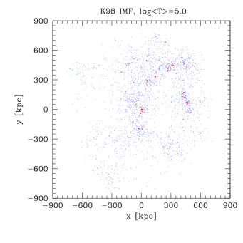
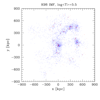
Figure 4: Spatial (projected) distributions of gas-phase oxygen in the “medium-density” field galaxy region, at $z$=3, for the K98 simulation. Results for 5 different temperature bins, corresponding to $\log(T)$=4, 4.5, .., 6, are shown. All temperature bins are represented using about 5000 “dots”, which for each temperature bin correspond to equal amounts of oxygen mass. Hence, each figure illustrates directly the spatial distribution of the gas-phase oxygen mass, not gas mass. The cold-phase ($\log(T)$=4) is shown by red dots in all 4 figures. In addition the $\log(T)$=4.5, 5, 5.5, and 6 phases are shown by blue dots in the corresponding panels.

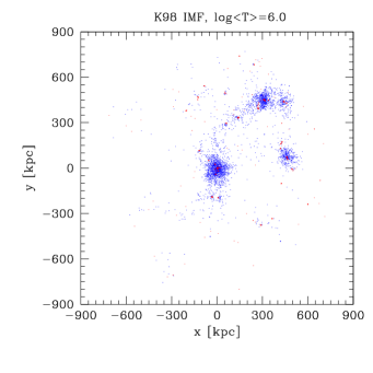
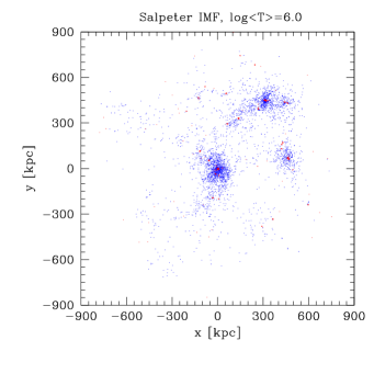
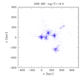
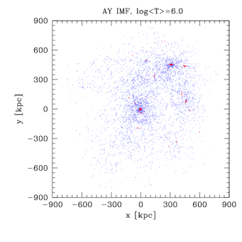
Figure 5: Spatial (projected) distributions of $\log(T)$=6 gas-phase oxygen in the “medium-density” field galaxy region, at $z$=3, for the K98 (top left), Salpeter (top right), AY (bottom right) simulations. Also shown is the result for a K98 simulation of a proto-elliptical region (bottom left) — see Fig. 4 for more detail

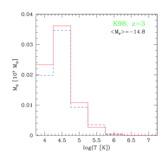
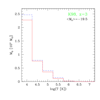
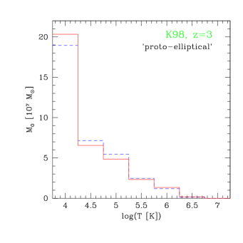
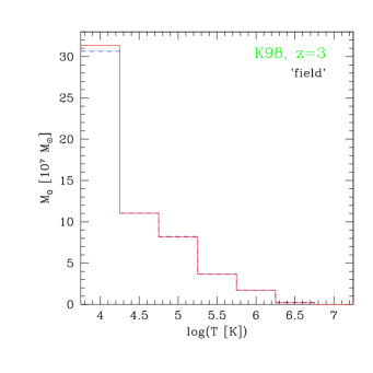
Figure 6: Comparison of predicted and actual gas-phase oxygen mass distributions for combinations of various regions simulated using the K98 IMF at high resolution. The top left plot shows the result for the combination of three regions, each containing a galaxy simulated using the “zoom-in” technique plus a number of companions. The three main galaxies have a mean $M_{\rm{V}}$ of $-14.8$. The red solid histogram shows the actual oxygen mass distribution of the three regions combined. The blue dashed histogram shows what the method outlined in the text predicts on the basis of the combined galaxy luminosity function of the three regions. The top right plot shows a similar comparison for a combination of 5 high-resolution regions containing main galaxies of an average $M_{\rm{V}}$ of $-19.5$. The bottom right plot is for the combination of the low and medium density “field” regions described in the text, containing a total of 103 resolved galaxies of $M_{\rm{V}}$ down to about $-22.5$. Finally, the bottom left plot shows the results for a higher density “proto-elliptical” region, containing 60 galaxies of $M_{\rm{V}}$ down to about -22.5.

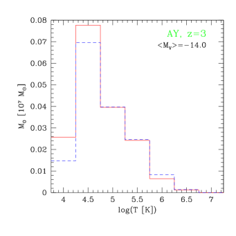
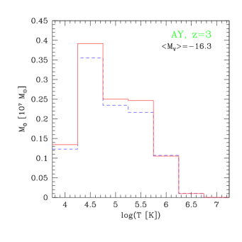
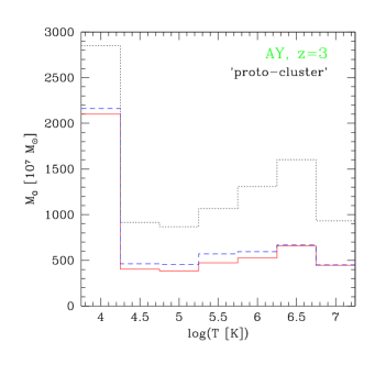
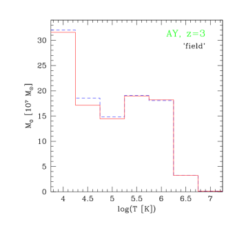
Figure 7: Similar to Fig. 6, but for simulations using the AY IMF. The top left plot shows the result for the combination of three regions, each containing a galaxy simulated using the “zoom-in” technique plus a number of companions. The three main galaxies have a mean $M_{\rm{V}}$ of $-14.0$. The top right plot shows results for a combination of 2 high-resolution regions containing main galaxies of an average $M_{\rm{V}}$ of $-16.3$. The bottom right plot is for the combination of the low and medium density “field” regions described in the text, containing a total of 40 resolved galaxies of $M_{\rm{V}}$ down to about $-21.5$. Finally, the bottom left plot shows the results for a very high density “proto-cluster” region, containing 86 galaxies of $M_{\rm{V}}$ down to about $-25.5$. The black dotted histogram shows the prediction using a constant $\tilde{r}$ approach (see text); the blue dashed histogram shows the prediction resulting from making the $M_{\rm{V}}<-22$ $\tilde{r}$ modification described in the text

3 The simulations

The code used for the simulations is a significantly improved version of the TreeSPH code we used for our previous work on galaxy formation (SGP03). A similar version of the code has been used recently to simulate clusters of galaxies, and a detailed description can be found in Romeo et al. (2006). Here we briefly mention its main features and the upgrades over the previous version of SGP03 — see also Sommer-Larsen (2006).

1. The basic equations are integrated by incorporating the “conservative” entropy equation solving scheme of Springel & Hernquist (2002), which improves the numerical accuracy in lower resolution regions.

2. Cold high-density gas is turned into stars in a probabilistic way as described in SGP03. In a star-formation event an SPH particle is converted fully into a star particle. Non-instantaneous recycling of gas and heavy elements is described through probabilistic “decay” of star particles back to SPH particles as discussed by Lia et al. (2002a). In a decay event a star particle is converted fully into a SPH particle, so that the number of baryonic particles in the simulation is conserved.

3. Non-instantaneous chemical evolution tracing 10 elements (H, He, C, N, O, Mg, Si, S, Ca and Fe) has been incorporated in the code following Lia et al. (2002a,b); the algorithm includes supernovæ of type II and type Ia, and mass loss and chemical enrichment from stars of all masses. Most of the simulations presented in this paper have been undertaken using three different Initial Mass Functions: the Kroupa (1998) IMF (denoted K98 in the following), derived for field stars in the Solar Neighborhood, the standard Salpeter IMF (S), and the more top-heavy Arimoto & Yoshii (1987) IMF (AY), which is well suited for the modeling of elliptical galaxies, as well as galaxy clusters. More detail is given in Lia et al. (2002a,b).

4. Atomic radiative cooling is implemented, depending both on the metallicity of the gas (Sutherland & Dopita 1993) and on the meta–galactic UV field, modeled after Haardt & Madau (1996). Moreover, a simplified treatment of radiative transfer, switching off the UV field where the gas becomes optically thick to Lyman limit photons on scales of $\sim$ 1 kpc, is invoked.

5. Star-burst driven winds are incorporated in the simulations at early epochs ($z$$\ga$5-6), as strong early feedback is crucial to largely overcome the angular momentum problem (SGP03). A burst of star formation is modeled in the same way as in SGP03: when a star particle is formed, further self-propagating star formation is triggered in the surroundings; the energy from the resulting, correlated SNII explosions is released initially into the interstellar medium as thermal energy, and gas cooling is locally halted to reproduce the adiabatic super–shell expansion phase; a fraction of the supplied energy is subsequently converted (by the hydro code itself) into kinetic energy of the resulting expanding super–winds and/or shells. The super–shell expansion also drives the dispersion of the metals produced by type II supernovæ (while metals produced on longer timescales are restituted to the gaseous phase by the “decay” of the corresponding star particles, see point 2 above).

   At later epochs, only a fraction (typically, 20%) of the stars induce efficient feedback, and star formation is no longer self–propagating so that no strong star-bursts are triggered by correlated SN explosions. This allows the smooth settling of the disc (see SGP03 for all details). Star formation efficiencies have been chosen such that realistic disc galaxy gas fractions result at $z$=0 (SGP03), and can also be shown to match the Kennicutt (1998) star formation relation quite well.

   AGN driven feedback has not been invoked in the simulations, as it is unlikely to play a major role in the formation of, at least, disc galaxies (e.g., Sommer-Larsen 2006) — the most common galaxy type in the Universe. The higher stellar UV escape fractions as well as LyC luminosities found by Razoumov & Sommer-Larsen (2007) at $z=3.6$, compared to $z\la 3$ , also support the notion that massive stars in galaxies become progressively more important sources of ionizing photons as one goes back in time, as the comoving number density of quasars declines rapidly at $z\raisebox{-3.8pt}{$\;\stackrel{{\scriptstyle\textstyle>}}{{\sim}}\;$}3$ (e.g., Richards et al. 2006). This provides additional circumstantial evidence that AGN feedback is of minor importance, at least at $z\ga 3$, the relevant redshift range in this paper.

The galaxies were drawn and re-simulated from a $10h^{-1}$ Mpc box-length dark matter (DM)-only cosmological simulation, based on the “standard” flat $\Lambda$ Cold Dark Matter cosmological model ($h=0.65$, $\Omega_{0}=0.3$, $\sigma_{8}=1.0$); our choice of $h$ and $\sigma_{8}$ is slightly different from presently more popular values (0.7 and 0.9 respectively), but this has little impact on the resulting galaxy properties (e.g., Portinari & Sommer-Larsen 2007). When re-simulating with the hydro-code, baryonic particles were “added” to the original DM ones, which were split according to an adopted baryon fraction $f_{b}=0.15$. The gravity softening lengths were fixed in physical coordinates from $z$=6 to $z$=0 and in co-moving coordinates at earlier times.

The simulations are run with resolutions of $m_{SPH}=m_{*}=3.6\times 10^{3}$-4.5$\times 10^{7}$ $M_{\odot}$, $m_{DM}=2.0\times 10^{4}$-3.3$\times 10^{7}$  $M_{\odot}$ and $\epsilon_{SPH}=\epsilon_{*}~{}=~{}0.08-3.8$ kpc going from the smallest individual galaxy simulations to the largest proto-cluster simulation. Each region containing an individual proto-galaxy was simulated using 0.2-2.2 million particles in total; in addition two “low” and “medium” galaxy density regions were simulated using 1.4 and 1.6 million particles, a proto-elliptical region using 1.4 million particles, and a proto-cluster region using 2.3 million particles (the high resolution “Virgo” simulation of Romeo et al. 2006).

Images of some of the simulated galaxies are available at http://www.tac.dk/$\sim$jslarsen.

4 The approach

The approach adopted is, based on the simulations, to characterize a given galaxy at $z$=3 and of absolute magnitude $M_{\rm{V}}$ by a distribution of ISM/IGM oxygen mass $m_{O}(M_{\rm{V}},\log(T))$, where $\log(T)$=3.5, 4, 4.5 , ..,7, and a given value of $\log(T)$ corresponds to gas temperatures in the range $T=[10^{\log(T)-0.25},10^{\log(T)+0.25}]$ K. Almost no oxygen is found at temperatures lower than 10^3.5 K, mainly because the radiative cooling function is effectively truncated below about 8000 K. If molecule formation and molecular cooling had been invoked in the hydro/gravity simulations, part of this gas would be in a much colder, high-density, predominantly H₂ phase (see also Sec. 8.1). Moreover, it is found that the $\log(T)$=3.5 as well as 4 ISM/IGM oxygen is spatially associated with the stellar galaxies (similar spatial extents), so the $\log(T)$=3.5 and 4 bins have been merged, and are denoted by $\log(T)$=4. Hence, all gas colder than 10⁴ K is included in this phase. Moreover, for field galaxies at $z$$\sim$3 almost no oxygen is found in the $\log(T)$$>$7 phases, which will therefore be ignored in the following.

Once the functions $m_{O}(M_{\rm{V}},\log(T))$ have been determined for a given IMF, the cosmologically averaged (gaseous) oxygen temperature distribution can be determined by folding these functions with the (dust corrected) rest-frame V-band luminosity function at $z\sim 3$. We stress that $m_{O}(M_{\rm{V}},\log(T))$ pertains only to the galaxy itself, not including any of its satellite galaxies — see further below.

To determine $m_{O}(M_{\rm{V}},\log(T))$ we proceed as follows: in Fig. 3 (left) is shown the cumulative mass of ISM/IGM oxygen, $M_{O}(r;M_{\rm{V}};\log(T))$, around three (mostly) isolated galaxies of $M_{\rm{V}}$ = $-16.1$, $-21.4$ and $-25.3$, respectively, simulated using the K98 IMF. Fig. 3 (right) is similar, but for the same three galaxies, of $M_{\rm{V}}$ = $-13.8$, $-19.3$ and $-25.4$, simulated with the AY IMF For all three galaxies the region from $r_{vir}$ to 8 $r_{vir}$ is shown, and the different curves correspond to $\log(T)$=4, 4.5 , ..,7. As can be seen from the figure, for a given galaxy and $\log(T)$, the cumulative gas oxygen mass gently increases with $r$ by factors $\sim$1.5-4, over the radial range shown. The one exception is the $\log(T)$=4 case, where the gas metals are mainly spatially correlated with the central galaxies, and the curves are quite flat (with the exception of the very bright galaxy, which has been selected from the proto-cluster simulations). We stress that the mass of gas-phase oxygen around a given (isolated) galaxy has been contributed not only by the stars in the galaxy itself, but also by stars in all its satellite galaxies (and in principle also by “inter-galactic” stars, as will be discussed below).

We select a sample of “base” galaxies consisting of (mainly) isolated galaxies ranging in absolute V-band magnitude from about $-12$ to $-25$. It is assumed that in order to account for the $m_{O}(M_{\rm{V}},\log(T))$ of a given base galaxy one should include all gas oxygen mass inside of a radius $\tilde{r}(M_{\rm{V}},\log(T))=r(M_{\rm{V}},\log(T))/r_{vir}(M_{\rm{V}})$, to be determined in the following, such that $m_{O}(M_{\rm{V}},\log(T))$=$M_{O}(\tilde{r}\times r_{vir};M_{\rm{V}};\log(T))$. “Isolated” galaxies are in this paper defined as galaxies not containing companions of stellar mass larger than 1/3 of the mass of the galaxy itself within 8 $r_{vir}$. The very brightest galaxies, however, of $M_{\rm{V}}$$\la-23$, were selected from the higher density proto-cluster simulations, and the criterion was relaxed to not containing companions of stellar mass larger than 1/2 of the mass of the galaxy itself within 4 $r_{vir}$. The relation between $r_{vir}$ and absolute V-band (rest-frame) magnitude $M_{\rm{V}}$ is shown in Fig. 2 for the three IMFs under consideration.

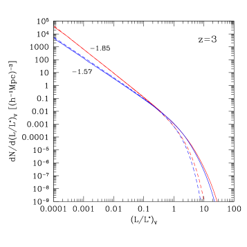
Figure 8: Observational and extinction corrected, modified V-band restframe galaxy luminosity functions, based on K-band observations by Shapley et al. (2001). Red dashed curve shows the original Shapley et al. LF of faint end slope $\alpha=-1.85$, red solid curve the corresponding extinction corrected, modified LF. Blue dashed curve shows the result of fitting a LF of faint end slope $\alpha=-1.57$ to the Shapley et al. data, blue solid curve the corresponding extinction corrected, modified LF.

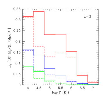
Figure 9: Cosmologically averaged gas-phase oxygen density temperature distributions for the three IMFs considered. Solid and dashed, green histograms correspond to the K98 IMF and the extinction corrected, modified galaxy luminosity functions of faint end slopes -1.85 and -1.57, respectively. The blue and red histograms show the corresponding quantities for the Salpeter and AY IMFs, respectively. For comparison, a density of 10⁷ $M_{\odot}$/$(h^{-1}\rm{Mpc})^{-3}$ corresponds to a density parameter of $\Omega_{O}=\rho_{O}/\rho_{\rm{crit}}=2.5\times 10^{-5}$, for $h$=0.7

For a given galaxy, $\tilde{r}$ will be finite for two reasons: a) no galaxy is perfectly isolated, such that, even for isolated galaxies, with increasing $\tilde{r}$ increasing amounts of gas-phase oxygen associated with other (smaller) companion galaxies are included, and b) for certain values of $\log(T)$ (depending on the IMF) galaxies are found to “share” a common pool of gas-phase oxygen. In practice it is found that for none of the IMFs considered, and any $\log(T)$, does $\tilde{r}$ exceed 8. For the brightest galaxies, $M_{\rm{V}}$$\la-23$, $\tilde{r}$ does not exceed 4.

Fig. 4 shows, for $\log(T)$=4.5, 5, 5.5 and 6, the spatial distribution of the gas-phase oxygen for a region containing 52 resolved galaxies with $M_{\rm{V}}$ in the range $-15$ to $-22.5$, simulated using the K98 IMF. Each dot represents, for a given $\log(T)$, an equal amount of gas-phase oxygen mass, so the figure displays the actual distribution of gas-phase oxygen mass, not gas mass. As can be seen, the spatial oxygen mass distributions depend strongly on the gas temperature.

In Fig. 5 is shown, for the three IMFs considered, the distribution of $\log(T)$=6 oxygen mass. As can be seen, the oxygen mass distribution also depends strongly on the IMF adopted. For comparison is also shown the corresponding plot for a K98 simulation of a proto-elliptical, high-density region, which is biased towards many large galaxies (bottom left) It is seen how the $\log(T)$=6 oxygen mass distribution in this case is concentrated near the large galaxies, more so than for the more representative “field” galaxy case.

We now approximate $\tilde{r}(M_{\rm{V}},\log(T))$ by $\tilde{r}(\log(T))$, i.e., independent of $M_{\rm{V}}$. We show further below that this is a good approximation, except for the very brightest galaxies, for which a correction has to be made. For each IMF, $\tilde{r}(\log(T))$ is determined as follows: i) for a number of regions containing up to about 200 resolved galaxies we a) determine the absolute V-band magnitudes of the $N$ galaxies in the region, $M_{V,1},...,M_{V,N}$, and b) the total gas-phase oxygen mass temperature distribution of the region

$$f_{O,\rm{region}}^{\rm{actual}}(\log(T))=\int_{region}\rho_{O}(\bar{x};\log(T))~{}d\bar{x}~{}~{}.$$ (2)

ii) for a given set of base galaxies, and given values of the $\tilde{r}(\log(T))$’s, one can predict the total mass of oxygen as a function of $\log(T)$ as

$$f_{O,\rm{region}}^{\rm{predicted}}(\log(T))=\Sigma_{i=1}^{N}M_{O}^{pred}(\tilde{r}\times r_{vir}(M_{V,i});M_{V,i};\log(T))~{}~{},$$ (3)

where $M_{O}^{pred}(\tilde{r}\times r_{vir};M_{V,i};\log(T))$ is determined by linear interpolation in $M_{\rm{V}}$ as well as $\tilde{r}(\log(T))$ ($\tilde{r}$=0,1,…8) using the corresponding values for the base galaxies. The values of $\tilde{r}(\log(T))$ are then obtained such as to provide the best simultaneous match of $f_{O,\rm{region}}^{\rm{predicted}}(\log(T))$ to $f_{O,\rm{region}}^{\rm{actual}}(\log(T))$ for a number of simulated regions, using standard least squares fitting.

For all three IMFs this is done for the same two regions, representing “low-density” and “medium-density” “field” environments, with galaxies of $M_{\rm{V}}\ga-22.5$. The two regions are simulated using a total of 1.4 and 1.6 million particles, respectively. For the AY IMF, two additional regions centered on smaller galaxies are also used (contrary to the K98 and S IMF cases, for the AY simulations such small galaxies have substantial amounts of not only $\log(T)$=4-6, but also $\log(T)$=6.5 and 7 gas-phase oxygen associated) — these regions are each simulated using about 300,000 particles in total. Finally, to test the approach also in a proto-cluster environment, for all three IMFs the same such region was simulated using a total of 2.3 million particles (the high-resolution “Virgo” region of Romeo et al. 2006).

As will be shown in the next section, in particular for $\log(T)$=4.5, 5 and 5.5, a significant contribution to the cosmic gas-phase oxygen budget comes from small galaxies with $M_{\rm{V}}\ga-17$ to $-19$. To check that the $\tilde{r}(\log(T))$ fits also work in this range, comparison was made to combined data-sets of regions with $M_{\rm{V}}$ of the central galaxy ranging from $-14$ to $-19$, all simulated at high resolution, with typically 200-300 000 particles per region. The results for the K98 IMF are shown in Fig. 6, including also the result for a proto-elliptical region. In general, the predicted distributions match the actual ones very well, except for the very smallest galaxies, where the predicted distribution falls somewhat short of the actual one in the $\log(T)$=4, 4.5 and 5 temperature bins. This implies that the results obtained in the following section for the faintest galaxies are actually lower limits. Given the small magnitude of the effect we shall, however, neglect this in the following.

In Fig. 7 a similar comparison is shown for AY IMF simulations. Again, the match between predicted and actual distributions is, in general, good. For the smallest galaxies the distributions are somewhat different (see above). For the proto-cluster region, the predicted distribution exceeds the actual one, with $f_{O,\rm{region}}^{\rm{predicted}}(\log(T))$ being up to about twice as large as $f_{O,\rm{region}}^{\rm{actual}}(\log(T))$. This is due to the very large galaxy density in such environments. Using this region to solve for an alternative set of $\tilde{r}(\log(T))$ results in $\tilde{r}(\log(T))$ values of about half the ones obtained as described above. As the main contribution to $f_{O,\rm{region}}^{\rm{actual}}(\log(T))$ is associated with the larger galaxies in the region, $M_{\rm{V}}\sim-24$ to $-25.5$, $f_{O,\rm{region}}^{\rm{actual}}(\log(T))$ in all regions can be matched by a model, where $\tilde{r}(\log(T))$ changes linearly from the “field” values to the “proto-cluster” values between $M_{\rm{V}}$ = $-22$ to $-24$, as shown in Fig. 6. However, in any case this correction for the very large galaxies is of no consequence to the main results presented in the following section. This is because the contribution from such galaxies to the overall cosmic metal budget is very minor, as will be detailed in the following section.

Finally we note, that even in typical “field” environments, some fraction of the stellar systems originally formed have subsequently been disrupted through tidal stripping and other dynamical processes. The gas-phase metals produced by these “inter-galactic” stars are “automatically” accounted for by the above approach, but in any case the fraction of such stars is quite small, $\la$5-10% (paper I).

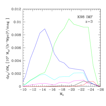
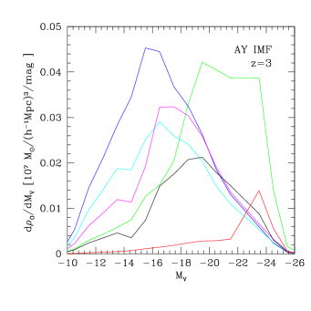
Figure 10: Contribution to cosmologically averaged gas-phase oxygen density as a function of galaxy V-band absolute magnitude for the K98 (left) and AY (right) IMFs. Curves corresponding to different gas temperatures are colour coded as in Fig. 3 ($\log(T)$=4: green, 4.5: blue, 5: cyan, 5.5: magenta, 6: black, 6.5: red). The results shown are for the extinction corrected modified Shapley et al. ($\alpha=-1.85$) galaxy luminosity function. For comparison with the cosmological density parameter, see caption of Fig. 9.

5 The temperature distribution of the cosmic gas-phase oxygen

The average cosmic density of gas-phase oxygen at $z$=3, as a function of gas temperature, can now be obtained as

$$\langle\rho_{O}(\log(T))\rangle=\int_{0}^{\infty}\frac{dN(L_{V})}{dL_{V}}~{}m_{O}(M_{\rm{V}}(L_{V}),\log(T))~{}dL_{V}~{}~{},$$ (4)

where $dN(L_{V})/dL_{V}$ is the rest-frame V-band, extinction corrected galaxy luminosity function at $z$=3.

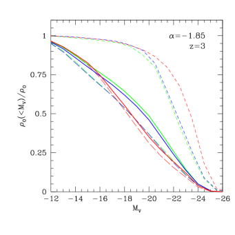
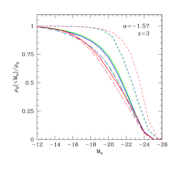
Figure 11: Fractional contribution to the cosmologically averaged gas-phase oxygen density by galaxies brighter than $M_{\rm{V}}$, for the extinction corrected modified Shapley et al. luminosity function (left) and the luminosity function of faint end slope -1.57 (right). Green, blue and red curves correspond to results for the K98, Salpeter and AY IMFs, respectively. Long-dashed curves correspond to gas-phase oxygen, short-dashed to stellar oxygen, and solid to the total.

In paper I the “true” $z\sim$3 galaxy luminosity function was determined by extinction correcting a modified version of the observationally determined luminosity function (LF) of Shapley et al. (2001) of faint end slope $\alpha=-1.85$. The original Shapley et al. (2001) LF, as well as the extinction corrected, modified LF, are shown in Fig. 8. Also shown are the corresponding LFs obtained by fitting a LF of faint end slope $\alpha=-1.57$ (see below) to the Shapley et al. (2001) data. The faint end slopes of these $z\sim 3$ LFs are steeper than what is found for $z\sim 0$ LFs. Results of semi-analytical galaxy formation models (e.g., Lacey et al. 2005) indicate that this is a natural outcome of hierarchical strucure formation scenarios.

Using the extinction corrected, modified Shapley et al. LF in eq. 4, and the $m_{O}(M_{\rm{V}}(L_{V}),\log(T))$ functions determined for the three IMFs as described in the previous section, results in the distributions shown in Fig. 9. For the K98 IMF, the amount of oxygen in the $\log(T)\geq$4.5 phase is about 1.1 times the amount in the $\log(T)$=4 “cold” phase. For the S and AY IMFs, the corresponding numbers are about 1.7 and 3.2, respectively. Hence, in particular, for the latter two IMFs, the majority of the gas-phase oxygen is in the “warm”/”hot” rather than cold phase. Moreover, for the AY IMF, the hot to cold/warm gas-phase oxygen mass ratio is 1.1, so the bulk of the oxygen is actually in the hot $\log(T)$$\ga$5 phase, rather than in the cold/warm phase. These are some of the main results of this paper.

In Fig. 9 is also shown the results of adopting a galaxy luminosity function with less steep faint end slope than the Shapley et al. one. Following paper I, results are presented for a luminosity function of faint end slope $\alpha=-1.57$, as found for the rest-frame UV $z\sim$3 luminosity function by, e.g., Adelberger & Steidel 2000). Although the results for this LF are qualitatively similar to the ones described above, the amounts of warm and hot phase oxygen decrease somewhat compared to the cold phase ones. The warm/hot to cold gas-phase oxygen mass ratios are for this LF 0.8, 1.1 and 2.1 for the K98, Salpeter and AY IMFs, respectively. Moreover, for the AY IMF, the hot to cold/warm gas-phase oxygen mass ratio is unity.

An obvious question is now: for the different gas temperatures, which galaxies contribute mainly to the cosmic gas-phase oxygen budget? In Fig. 10 this is shown using the modified Shapley et al. luminosity function, for the K98 and AY IMFs, respectively. It is seen that for the K98 IMF the main contribution to the $\log(T)$=4.5 phase comes from small galaxies, $M_{\rm{V}}\sim-16$, and for the AY IMF this is the case for the $\log(T)$=5 and 5.5 phases as well (the reason for the large difference between the $M_{\rm{V}}$-distributions of $\log(T)$=4 and $\log(T)$=4.5, say, gas-phase metals is that, whereas the $\log(T)$=4 gas is of fairly high density and associated with all galaxies, $\log(T)$=4.5 gas is typically diffuse and associated with halos of comparable virial temperature, i.e. fairly small galaxies).

Given this, and in relation to observational studies, it is clearly of interest to determine how large a fraction of the gas-phase oxygen is associated with galaxies to a certain limiting magnitude. In Fig. 11 this is shown by the long-dashed curves (for the three IMFs considered) for the $\alpha=-1.85$ and $-1.57$ LFs. Typical Lyman Break galaxy metallicity determinations at $z\sim$3 only probe to about one magnitude below $L^{*}$, i.e., $M_{\rm{V}}\sim-22$. For the $\alpha=-1.85$ LF, it is found that less than about 20% of the cosmic gas-phase oxygen will be associated with galaxies brighter than this, irrespective of the choice of IMF. For the $\alpha=-1.57$ LF the corresponding fraction is about 30%. Hence, most of the cosmic gas-phase oxygen is associated with galaxies considerably fainter than $L^{*}$, and is also in this sense “missing”.

In calculating the results shown in Fig. 11 it has been assumed that the observational LFs maintain a constant faint end slope down to $M_{\rm{V}}=-10.5$. As can be seen from the figure, in particular for the $\alpha=-1.85$ case this is somewhat critical to the shape of the curves shown. At redshifts $z$$\sim$3 the LBGs luminosity function is only probed down to a few magnitudes below $L^{*}$ (but see below). Selecting galaxies using the Ly$\alpha$ line it is possible to probe 2-3 magnitudes fainter still (Fynbo et al. 2001, 2003; Gawiser et al. 2006; Nilsson et al. 2007). This, however, only demonstrates the existence of star-forming galaxies at these redshifts with M${}_{V}\sim-17$ to $-18$, but the data are not good enough to put strong constraints on the shape of the luminosity function. Jakobsson et al. (2005) find that the magnitudes of $z>2$ GRB selected galaxies are consistent with being drawn from the steep luminosity function, but the statistics are still poor. We note, however, that Bouwens et al. (2007) were actually able to probe the UV luminosity function at $z\sim 4-6$ down to 4-5 magnitudes below $L^{*}_{UV}$ and find steep faint end slopes, $\alpha\sim-1.7$.

Our calculations show, however, that if the slope of the faint end LF flattens significantly at some brighter $M_{\rm{V}}$, then the curves still fairly well represent the result, after appropriate renormalisation at this limiting $M_{\rm{V}}$ (if the faint end slope is assumed to be constant to even fainter than $M_{\rm{V}}=-10.5$, the results are not much changed compared to the $M_{\rm{V}}=-10.5$ results). Moreover, we note that neither the Two-Degree Field Galaxy Redshift Survey (2dFGRS) $b_{j}$ local luminosity function (Norberg et al. 2002), nor the Sloan Digital Sky Survey (SDSS) U-band local luminosity function (Baldry et al. 2005) show any flattening of the faint end slope to 5-6 magnitudes fainter than $M_{*}$. Moreover, some galaxy cluster luminosity functions tend to show a steepening faint end slope: Milne et al. (2007) find a steepening of the slope in the Coma cluster at a $M_{R}$ range of about $-14$ to $-9$, and Yamanoi et al. (2007) find a similar result for the Hydra I cluster.

Given the significance of the results obtained in this section on the distribution of cosmic gas-phase metals, it is important to consider the following two sources of potential model dependence.

First, it is possible that the results depend on the specific choice of “base” galaxies. We verified explicitly, however, that choices of alternative sets of isolated sets of “base” galaxies, and subsequently going through the procedure described in the previous section, lead to very similar results as the ones described here. Hence, the results presented are very robust to this.

Second, it would be expected that the amount of (in particular) $\log(T)$=4 cold gas and metal mass available in a simulation at any given time would depend on the star-formation efficiency adopted (Sec. 3). To this end, three K98 galaxy simulations, of galaxies of $z$=3 $M_{\rm{V}}$=$-19.1$, $-21.5$, and $-22.3$ and surrounding regions, were run with twice the standard star-formation efficiency. Comparing the results of these simulations to the corresponding standard ones, it was found that the total mass of gas-phase oxygen at $z$=3 was virtually unchanged, and that the mass of $\log(T)$=4 oxygen was reduced by $\la$5-10% compared to the standard case. Hence, none of the main conclusions about $\log(T)$=4 metals, obtained in this and the following sections, are affected by such a change. Moreover, a doubling of the star-formation efficiency would lead to too small $z$=0 disc galaxy gas fractions, and likely also too small disc galaxy angular momenta (SGP03), likely too small $z$$\sim$3 DLA cross-sections (Ellison et al. 2007, Sommer-Larsen et al. 2007), and star-formation rates above the Kennicutt (1998) relation.

6 C iv properties of the low to intermediate density IGM

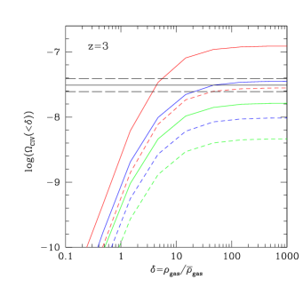
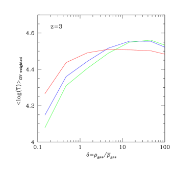
Figure 12: Cumulative cosmic C iv density, in units of the critical, $\Omega$(C iv) as a function of the gas over-density $\delta=\rho_{\rm{gas}}/\bar{\rho}_{\rm{gas}}$ (left). Green, blue and red curves correspond to the K98, Salpeter and AY IMFs. Solid curves corresponds to upper limits, dashed to lower. Also shown, as a horizontal, black solid line, is the median of ten observational estimates at redshifts in the range 1.5-4.5 taken from Songaila (2001), Boksenberg, Sargent & Rauch (2003) and Songaila (2005). Horizontal black dashed lines show 1-$\sigma$ deviations, where $\sigma$ is the variance of the observational estimates. The plot to the right shows the median C iv abundance weighted temperature of the IGM as a function of gas over-density, for the three IMFs.

Interesting tests of the abundance and thermal properties of the low to intermediate density IGM are provided by OSO absorption line studies of the Lyman metal forest, as probed by C iv. Songaila (2001) first determined $\Omega$(C iv) by integrating the total column density of systems between $10^{12}\leq N$(C iv)$<10^{15}$ cm^-2 — see also Schaye et al. (2003). As shown by, e.g., OD06, this range of column densities trace moderate IGM gas over-densities, $\delta=\rho_{gas}/\bar{\rho}_{gas}\sim 1-100$, or $n_{\rm{H}}\sim 10^{-5}-10^{-3}$ cm^-3, at $z$$\sim$3. To obtain a corresponding estimate of $\Omega$(C iv) based on our simulations we adopted the following approach:

To convert from total C (as given in our simulations) to C iv abundances, ionisation corrections are required. We base our conversion on ionisation corrections determined by OD06 using CLOUDY (Ferland et al. 1998). OD06 assumed the Haardt & Madau (2001) $z$$\sim$3 UV background field divided by a factor 1.6 at all redshifts, in order to match the observed mean Ly$\alpha$ flux decrement, $D_{Ly\alpha}$. This may seem inconsistent with our use of the Haardt & Madau (1996) UVB in the cosmological simulations, but as shown by Croft et al. (1998), because photo-ionisation is sub-dominant in gas dynamics such a correction yields virtually identical results as having done the simulations with the above (reduced) background. The resulting ionisation corrections were kindly supplied to us by Ben Oppenheimer and Romeel Davé, in the form of look-up tables.

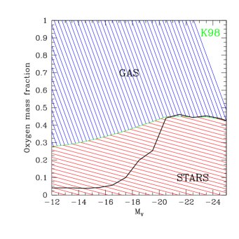
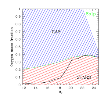
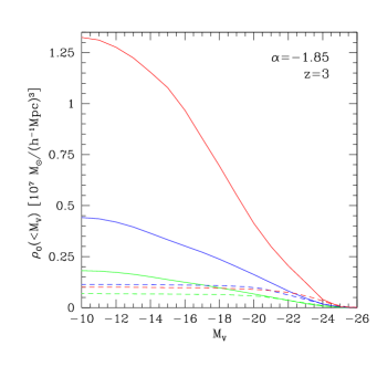
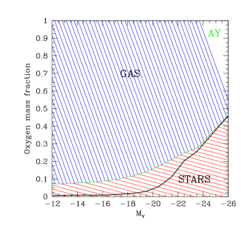
Figure 13: Cumulative fractional contributions of oxygen mass in stars and gas, up to a given $M_{\rm{V}}$, are shown by the green solid lines, separating the red and blue hatched regions (stellar/gas-phase oxygen). All results are for the $\alpha=-1.85$ LF, and the plots shown are for the K98 (top left), Salpeter (top right) and AY (lower right) IMFs. Also shown in these plots, by black solid lines, is the fractional partition between oxygen mass in stars and gas at any given $M_{\rm{V}}$. Finally, in the lower left plot is shown the cumulative cosmic oxygen density in gas+stars (solid lines) and stars only (dashed lines). In this plot the IMFs are colour coded as follows: green: K98, blue: Salpeter, red: AY. For comparison with the cosmological density parameter, see caption of Fig. 9.

In Fig. 12 (left) is shown the cumulative $\Omega$(C iv) as a function of $\delta$. For the two simulated “field” galaxy regions the average ratio of the cumulative C iv mass to total (gas-phase) oxygen mass has been determined. This has then been multiplied by $\Omega_{O,gas}$, determined on the basis of the results obtained in the previous section. As is clear from this section, the value of $\Omega_{O,gas}$ depends on the actual form of galaxy luminosity function. To obtain lower and upper limits on $\Omega_{O,gas}$, we evaluate it at $M_{\rm{V}}$=$-21$ and $-10$, respectively, assuming the $\alpha=-1.85$ luminosity function. $M_{\rm{V}}$=$-21$ corresponds approximately to the detection limit of Shapley et al. (2001), whereas $M_{\rm{V}}$=$-10$ corresponds to assuming that the faint end slope remains constant to this very faint magnitude. As can be seen from Fig. 11, using the $\alpha=-1.57$ LF provides less conservative limits. In the figure is shown the result of applying the lower and upper limits for the K98, Salpeter and AY IMFs, respectively. Using other simulated regions, centered on smaller galaxies, yields similar results. Using the proto-cluster region to determine the average ratio of the cumulative C iv mass to total (gas-phase) oxygen mass results in lower values of $\Omega$(C iv), due to the temperature dependence of the C/C iv ionisation correction combined with the higher average IGM temperature of the proto-cluster region. However, proto-cluster regions are very special sites, and, as can be seen from the results of the previous section, the contribution to the cosmic metal production associated with the very luminous galaxies typical of such regions, $M_{\rm{V}}\sim-25$, is very small (in the proto-cluster regions containing 100-200 galaxies, almost half of the gas-phase metals are associated with five galaxies of $M_{\rm{V}}\la-24$). Also shown in the figure is the median value of 10 observational estimates in the redshift range $z$=2-4, where the run of observed $\Omega$(C iv) with redshift is essentially flat (e.g., Songaila 2001, Schaye et al. 2003, Songaila 2005), as well as the observational variance. The observational estimates were taken from Songaila (2001), Boksenberg, Sargent & Rauch (2003) and Songaila (2005).

As can be seen, the chemical yield of the K98 IMF appears too low to match the observational estimates, whereas the Salpeter and AY IMFs can match the observations, and an IMF with a yield in between these two appears optimal. We caution, however, that our estimates of $\Omega$(C iv) depend on the adopted gas-phase oxygen to C iv mass conversions. The optimal would be to carry out simulations of $\ga$100 $h^{-1}$Mpc box size cosmological volumes at the (high) resolution of our galaxy formation runs, but as mentioned previously, this is currently computationally prohibitive. Hence, our result above on the cosmic IMF should be seen as indicative only. The main point is that both the Salpeter and AY IMF simulations can match the observational constraints on $\Omega$(C iv).

Observations of C iv line widths for the above column density range can be used to probe the thermal properties of the low-density IGM. Three components contribute to the line widths: a) thermal broadening, b) spatial broadening due to Hubble expansion across the physical extent of the absorber, and c) turbulent broadening. The last component can be ignored, since the IGM at these over-densities is very quiescent (Rauch et al. 2005). Observational estimates of C iv line widths by Boksenberg, Sargent & Rauch (2003) indicate $b\simeq$10 km/s in the range $z\sim$1.5-4.5 for $10^{13}\leq N$(C iv)$<10^{14}$ cm^-2 absorbers. This can be used to derive upper limits to the C iv abundance weighted IGM temperature. As the thermal component of the C iv line width is given by $b_{th}=3.7\sqrt{T/10^{4}}$, C iv abundance weighted IGM temperatures of less than $\sim$5$\times$10⁴ K are indicated. In Fig. 12 (right) we show C iv abundance weighted IGM temperatures a function of $\delta$ in the “field” galaxy regions for the three IMFs considered (results for other regions are quite similar). It is seen that models in general satisfy the above IGM temperature criterion. Moreover, our predictions of the abundance weighted IGM temperatures agree well with the predictions of OD06 for their best fitting “momentum-driven” wind model.

Finally we note, that in the future it will be possible to probe the metal enrichment of the IGM to even lower densities using O vi— see, e.g., Schaye et al. (2000).

7 Combining the cosmic stellar and gas-phase oxygen distributions

With the results on the cumulative cosmic gas-phase oxygen distributions presented in the previous section, and the results on the similar distributions for the stellar oxygen from paper I, we can now assess the relative importance of the two components. In Fig. 11 results for the normalised gas-phase oxygen distributions are shown by long-dashed curves, the stellar distributions are shown by the short-dashed curves, and the combined distributions by the solid curves (for the three IMFs considered) for the $\alpha=-1.85$ and -1.57 LFs (we note that stellar oxygen refers to oxygen in galactic stars only, but since the amount of oxygen in intergalactic stars is, in comparison, very small (paper I), we neglect this component in the following).

As can be seen, the combined distributions are for all three IMFs dominated by the gas-phase oxygen, and increasingly so going from the K98 to the AY IMF. For the $\alpha=-1.85$ LF, it is found that less than about 25% of the total cosmic oxygen is associated with galaxies brighter than $M_{\rm{V}}=-22$, irrespective of the choice of IMF. For the $\alpha=-1.57$ LF the corresponding fraction is about 35% for the AY IMF, and about 40% for the K98 and Salpeter IMFs.

Fig. 13 shows, for the $\alpha=-1.85$ luminosity function, and the three IMFs, the cumulative partition between gas-phase oxygen and stellar oxygen as a function of $M_{\rm{V}}$. It is seen, that if the faint end slope of -1.85 holds down to $M_{\rm{V}}\sim-12$, then the cumulative gas-phase oxygen fractions are 72, 79 and 92% for the K98, Salpeter and AY IMFs, respectively, so, as stated above, for all three IMFs, the amount gas-phase oxygen dominates over the amount stellar oxygen. For the $\alpha=-1.57$ luminosity function these fractions drop slightly to 64, 71 and 88%.

As discussed in Sec. 5 the calculations assume a constant faint end slope down to $M_{\rm{V}}$=$-10.5$. If the luminosity function is assumed to display a significant flattening at a brighter magnitude than this, then the figure can still be used to determine the gas-phase/stellar oxygen partition to such a limiting $M_{\rm{V}}$. Assuming, for example, that the faint end slope is constant to at least 6 magnitudes below $M^{*}$ (i.e., $M_{\rm{V}}$$\sim-17$), which is the case for local luminosity functions (Sec. 5), results in lower limits on the cumulative gas-phase oxygen fractions of 65, 72 and 90% for the $\alpha=-1.85$ luminosity function, i.e., not much different from the results quoted above.

We can now finally compare the integral constraints on the average cosmic oxygen density at $z$=3, obtained in Sec. 2, to what is obtained by combining detailed high-resolution galaxy formation simulations with the observed (corrected) $z$$\sim$3, V-band luminosity function. In Fig. 14 we show the cumulative oxygen density versus $M_{\rm{V}}$ for the three IMFs and the two faint end luminosity function slopes considered. Also shown are the constraints from the “minimum”, “median” and “maximum” oxygen production rate density models discussed in Sec. 2. In order to enable a meaningful comparison, the latter results should be compared to the former evaluated at certain limiting magnitudes. These magnitudes should be chosen to be brighter than or equal to about $M_{\rm{V}}\simeq-21.0$, $-20.5$ and $-20.0$ for the K98, Salpeter and AY IMFs, respectively, for the following reasons:

Kennicutt (1998) finds a relation between UV luminosity and star formation rate (SFR), viz.

$$SFR~{}(M_{\odot}\rm{yr}^{-1})=1.4\times 10^{-28}~{}\beta_{\rm{IMF}}~{}L_{\nu}(\rm{ergs}~{}\rm{s}^{-1}\rm{Hz}^{-1}),$$ (5)

with $\beta_{\rm{IMF}}$=1.0 for the Salpeter IMF. Given that the yield of the Kroupa (1998) IMF is smaller than for the Salpeter IMF, and vice versa for the Arimoto-Yoshii IMF, $\beta_{\rm{IMF}}$ will be larger and smaller than unity for these two IMFs, respectively. Quantitatively we find that $\beta_{\rm{IMF}}\simeq$1.7 and 0.4 for the K98 and AY IMFs, respectively.

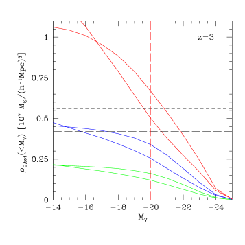
Figure 14: Contribution to the cosmologically averaged total (gas-phase and stellar) oxygen density by galaxies brighter than $M_{\rm{V}}$, for the modified Shapley et al. luminosity function, and the luminosity function of faint end slope -1.57. Green, blue and red curves correspond to results for the K98, Salpeter and AY IMFs, respectively. (for comparison with the cosmological density parameter, see caption of Fig. 9). In the right side of the plot, the $\alpha=-1.57$ curves are above the corresponding $\alpha=-1.85$ ones. Also shown, by horizontal dashed lines, are the constraints from the integrated cosmic oxygen production history derived in Sec. 2. Finally, the lower V-band luminosity limits, at which the predictions for the various IMFs and LFs should be compared to the integral constraints, are shown by green, blue and red vertical dashed lines for the K98, Salpeter and AY IMFs, respectively — see text for details.

The absolute UV magnitude ($\lambda\sim$1500 Å) characterising the observed galaxy luminosity function at $z$$\sim$3 (i.e., corresponding to $L^{*}_{UV,z=3}$) is $M^{*}_{UV,z=3}$$\simeq-21.0$ (e.g., Steidel et al. 1999, after correction to the adopted cosmology, Sawicki & Thomson 2006). Following Sawicki & Thomson (2006), and using eq. 5 above, one can show that this absolute magnitude corresponds to a (un-extincted) star formation rate of about 15 $\beta_{\rm{IMF}}$ $M_{\odot}$/yr. With a dust correction of about a factor 5.5 at $z$$\sim$3 (Sec. 2) the above observed $M^{*}_{UV,z=3}$ hence corresponds to a true (un-obscured) SFR of about 82 $\beta_{\rm{IMF}}$ $M_{\odot}$/yr. We shall now consider two models for the $\lambda\sim$1500 Å extinction as a function of redshift for $z\geq$3. Model A assumes a constant extinction factor of 5.5 at all $z\geq$3 (cf. Sec. 2), whereas model B is a low-extinction model assuming factors of 4.2, 3, 2 and 1.5 at $z$=3, 4, 5 and 6, respectively (cf. Bouwens et al. 2006). For model A, a galaxy of observed $L_{UV}=0.1\times$$L^{*}_{UV,z=3}$ will be characterised by a SFR$\sim$8 $\beta_{\rm{IMF}}$ $M_{\odot}$/yr. From our large sample of galaxy models we find that galaxies with such star formation rates at any $z\geq$3 will have an (un-extincted) $M_{\rm{V}}$ at $z$=3 brighter than about $-22.0$, $-21.5$ and $-20.5$ for the K98, Salpeter and AY IMFs, respectively. For model B, the above $M^{*}_{UV,z=3}$ corresponds to a true SFR of about 63 $\beta_{\rm{IMF}}$ $M_{\odot}$/yr, and galaxies of observed $L_{UV}=0.1\times$$L^{*}_{UV,z=3}$ will have SFRs of about 6.3, 4.5, 3.0 and 2.3 $M_{\odot}$/yr at $z$=3, 4, 5 and 6, respectively. We find that only galaxies of (un-extincted) $M_{\rm{V}}$ at $z$=3 brighter than about $-21.5$, $-21.0$ and $-20.5$ for the above three IMFs, respectively, will satisfy this. Moreover, even assuming (very conservatively) zero extinction at $z\ga$6, corresponding to a “limiting” (un-extincted) SFR of about 1.5 $M_{\odot}$/yr, all galaxies of such $z\ga$6 SFRs will be be brighter than about $M_{\rm{V}}$=$-21.5$, $-21.0$ and $-20.5$ at $z$=3 for the three IMFs, respectively. Assuming lower luminosity limits of $M_{\rm{V}}$=$-21.0$, $-20.5$ and $-20.0$ for the three IMFs is hence very conservative — these limits are indicated in Fig. 14 by vertical dashed lines.

From Fig. 14 it follows that galaxy models based on the K98 IMF can not meet the constraint set by the observed UV luminosity density history — the oxygen (and general metal) yield of this IMF is simply not sufficiently large. The same is the case for the Salpeter IMF, though the $\alpha=-1.57$ model comes close to matching the lower bound of 0.32$\times 10^{7}$ $M_{\odot}$/($h^{-1}$Mpc)³ (see also below). On the other hand, models based on the Arimoto-Yoshii IMF, match the integral constraint well.

Summarising, one of the main results obtained in this paper is that galaxy formation models based on the Kroupa (1998) IMF (and any other IMF of similar chemical yield) are strongly excluded by the cosmic enrichment history constraint. Other arguments, why the average cosmic IMF must have a larger chemical yield than what is typical for a solar neighborhood one, have been given by, e.g., Portinari et al. (2004), D’Antona & Caloi (2004), Serjeant & Harrison (2005), Lucatello et al. (2005), Loewenstein (2006), Prantzos & Charbonnel (2006) and Weidner & Kroupa (2006), but see also Elmegreen (2006).

Perhaps even more interestingly, models based on the Salpeter IMF, the arguably most extensively used model of the stellar IMF, are also excluded, though the $\alpha=-1.57$ models only marginally so. Given that the Salpeter IMF is routinely used in translating UV luminosities into star formation rates for high redshift galaxies, this is also an important result. Although it would be inappropriate to assign a high statistical significance to this result, given all the uncertainties involved, it is obvious from Fig. 14 that the models based on the more top-heavy Arimoto-Yoshii IMF provide a much better match to the median value for the integral constraint. This is in particular the case, since the above lower absolute luminosity limits of $M_{\rm{V}}$=$-21.0$, $-20.5$ and $-20.0$ for the three IMFs, respectively, are likely to be very conservative.

8 Missing metals and comparison to other works

In Sec. 5 it was shown that for the $\alpha=-1.85$ $z$$\sim$3 luminosity function, less than about 1/4 of the cosmic oxygen is associated with Lyman Break galaxies sufficiently bright, $M_{\rm{V}}$$\ga-22$, for direct abundance determination, using oxygen lines emitted from HII regions around young stars in the galaxies (e.g., Pettini et al. 2001). For the $\alpha=-1.57$ luminosity function this fraction increases slightly, to about 35%. Furthermore, in Sec. 7 it was shown that for both luminosity functions the major part of the cosmic oxygen is in the gas-phase, rather than in stars. In particular, for the Salpeter and Arimoto-Yoshii IMFs, which emerge from the previous section as the more plausible, the gas-phase oxygen fraction exceeds 70%.

FSB05 found a factor of about five discrepancy between the amount of metal in the stars of Lyman Break galaxies and what is predicted from the integrated UV luminosity density history. They assumed typical Lyman Break galaxy stellar masses of 2 $\times 10^{10}$ $M_{\odot}$, corresponding to $M_{\rm{V}}$$\sim-22.5$, i.e., close to $M^{*}_{V,z=3}$.

In Fig. 13 is shown, for the $\alpha=-1.85$ luminosity function, the cumulative stellar cosmic oxygen density. For the K98 IMF, the ratio between the stellar oxygen density to $M_{\rm{V}}=-21$ and what is obtained from the median model (Sec. 7) is 0.10. For the Salpeter and AY IMFs, evaluated at $M_{\rm{V}}=-20.5$ and $-20$, respectively, the corresponding ratios are 0.17 and 0.20. For the $\alpha=-1.57$ luminosity function the corresponding ratios are 0.14, 0.24 and 0.29, for the K98, Salpeter and AY IMFs, respectively. Given that the AY models over-predict the metallicities of Lyman Break galaxies of $M_{\rm{V}}\sim-22$ to $-23$ by about 0.2 dex relative to observations (paper I), the above ratios for the AY models should be reduced to 0.13 and 0.18 for the $\alpha=-1.85$ and -1.57 luminosity functions, respectively.

The above results are obtained, however, by including stellar oxygen mass all the way down to $M_{\rm{V}}$$\sim-20.5$. If one only includes stellar oxygen mass to $M_{\rm{V}}$$\sim-22.5$, all the above fractions are reduced by about a factor of two. Hence the discrepancy discussed above, denoted by FSB05 and others as “the missing metals problem”, is actually about twice larger than originally found by FSB05.

DO06 predicted that at $z$$\sim$3, about 50% of the gas-phase metals should reside in the diffuse IGM (gas outside the virial radii of galaxy halos, and of $T<3\times$10⁴ K). We can not compare the results found in the previous sections directly to theirs, since different gas-phase criteria have been used. However, our $\log(T)$=4.5 gas criterion is similar to theirs for diffuse IGM, though we also include $\log(T)$=4.5 metals inside of galaxy virial radii in our estimate (see also below; note also that we find almost all the $\log(T)$=4 phase metals to reside in gas of fairly high density, $n_{\rm{H}}$$\ga$0.1 cm^-3, so there is essentially no overlap between this phase and DO06’s diffuse phase).

For the $\alpha=-1.85$ LF we find $\log(T)$=4.5 to total gas phase metal fractions of 34, 31 and 26% for the K98, Salpeter and AY IMFs, respectively. For the $\alpha=-1.57$ LF, the corresponding fractions are 21, 20 and 18%. If we try to mimick the criterion of DO06 better, by selecting all metals in gas of $T$$<$3$\times$10⁴ K and $\delta=\rho_{gas}/\bar{\rho}_{gas}$$\leq$100, then for the field galaxy regions we find “diffuse IGM” oxygen fractions of 4, 4 and 6% for the K98, Salpeter and AY IMFs, respectively. If we use the proto-cluster regions, which are the only simulations at our disposal with a resolution comparable to the (fairly modest) numerical resolution of DO06’s 32 $h^{-1}$Mpc box size simulation, the corresponding fractions drop to $\sim$1% for all IMFs. However, we stress that the temperature of the proto-cluster IGM is larger than that of the average IGM, but in any case significantly lower “diffuse IGM” metal fractions, than predicted by DO06, are indicated.

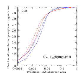
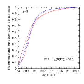
Figure 15: Left: Fractional cumulative oxygen mass in the absorbers above log(N(HI))=20.3 versus the cumulative absorber area, starting at the highest HI surface densities. Red and blue curves correspond to the proto-galaxies of $z$=0 $V_{c}$=245 km/s and 180 km/s, respectively. “Face-on” projections are shown by solid and “edge-on” by dashed curves. Center: Same, but versus HI column density. Right: Oxygen and iron abundance versus HI column density; for clarity only “face-on” projections are shown. Red and blue curves show [O/H], green and cyan [Fe/H].

DO06 used the Springel & Hernquist (2003) “sub-grid” approach to model star-formation. They predict that about 20% of the gas-phase metals reside in star-forming gas. In our models, which invoke explicit two-phase modeling of the ISM, gas of $T$$\sim$$10^{4}$ K and $n_{H}$$\ga$0.1 cm^-3 is potentially star-forming. Hence we compare our results for the $\log(T)$=4 gas-phase metal content to the above of DO06 (as noted above, almost all $\log(T)$=4 metals reside in gas of $n_{H}$$\ga$0.1 cm^-3). For the $\alpha=-1.85$ LF we find $\log(T)$=4 to total gas phase metal fractions of 47, 37 and 26% for the K98, Salpeter and AY IMFs, respectively. For the $\alpha=-1.57$ LF, the corresponding fractions are 57, 47 and 32%. Hence we find somewhat larger metal fractions in star-forming gas, than do DO06. A more important difference is, however, that DO06 at $z$$\sim$3 find no metal containing gas at densities $n_{H}$$\ga$0.01 cm^-3. This result is strongly at variance with our results, and it would seem difficult for such models to match the large amount of DLA cross section observationally detected at such redshifts, although further analysis obviously is required to clarify this.

Finally, we can compare the $z$=3 gas phase metal temperature distribution predicted by DO06 to our results. Qualitatively, our predictions for the K98 and Salpeter IMFs agree with that of DO06, in yielding temperature distributions, which peak at $T$$\sim$$10^{4}$ K and decrease towards larger temperatures. However, for the AY IMF the results are very different. Moreover, quantitatively our results for the K98 and Salpeter IMFs disagree significantly with those of DO06 at the “high-$T$” end: DO06 find that $\la$5% of the gas-phase metals reside in gas of $T$$>$$10^{4.75}$ K. In comparison, we find for the $\alpha=-1.85$ LF that the corresponding fractions are 20, 32 and 51% for the K98, Salpeter and AY IMFs, respectively, and for the $\alpha=-1.57$ LF, 21, 32 and 50%. Hence for any of the IMFs considered, we predict significantly larger fractions of “high-$T$” gas-phase metals, than do DO06.

8.1 Metals in the cold gas-phase and DLA absorbers

The $\log(T)$=4 phase is found to be the most prominent metal containing gas-phase for the K98 and Salpeter IMFs, and also to be quite prominent for the AY IMF. As the metals in this phase typically reside in gas of densities $n_{H}$$\ga$0.1 cm^-3, one would expect a significant fraction of these metals to be situated at column densities typical of DLAs, viz. N(HI)$\geq$10^20.3 cm^-2. However, in general DLAs have very low abundances - significantly less than Galactic stars with similar ages (Pettini et al. 1990, 1994; Lu et al. 1996; Kulkarni & Fall 2002; Prochaska et al. 2003; Akerman et al. 2005; Zwaan et al. 2005; Erni et al. 2006). Expressed in terms of the global metal content of the LBG stars, we predict similar to three times as large amounts of metals in the $\log(T)$=4 phase (depending on the IMF), whereas observations of DLAs only indicate a fraction of about 10-20% (e.g., FSB05, Prochaska et al. 2006). It is obviously of importance to understand the reason for this apparent discrepancy. Although we will defer a thorough discussion of DLAs to a forthcoming paper (Sommer-Larsen et al. 2007), we briefly address the above issue in the following.

Ellison et al. (2007) analysed two of the very high resolution simulations, described in the following section, in relation to DLA properties. The two simulations represent the formation and evolution of two disc galaxies, of $z$=0 characteristic circular velocities $V_{c}$=245 and 180 km/s. The galaxies were selected from a larger sample to represent two different disc formation evolutionary paths: for the $V_{c}$=180 km/s galaxy the disc starts growing steadily already by $z$$\sim$2.5, whereas for the other galaxy disc growth is merger induced, and the disc grows strongly from $z$$\sim$1 to 0 (see also Robertson et al. 2004). Ellison et al. determined the DLA/sub-DLA characteristics of these two proto-galaxies at $z$=3.6, 3.0 and 2.3, with focus on determining neutral column density distributions, and the probability of detecting coincident 100 kpc-scale DLA/sub-DLA absorption in individual galaxies at such redshifts — we refer the reader to Ellison et al. for more detail, as well as images of the objects.

Here we build on the analysis by Ellison et al. of these two (proto-)galaxies. In Fig. 15 (left) we show the normalised cumulative oxygen mass in the absorber above log(N(HI))=20.3 versus the cumulative absorber area, starting at the highest HI surface densities, log(N(HI))$\sim$24, and going down to log(N(HI))=20.3. For each galaxy results for “face-on” and one “edge-on” projections are shown. As can be seen, about 90% of the total oxygen mass of the absorber resides in 1% of the total absorber area for both projections. From Fig. 15 (center) it is moreover seen that this oxygen mass is associated with column densities log(N(HI))$\ga$22.5. DLAs of such high column densities have never been detected in QSO spectra, which of course is not surprising given the above findings. Moreover, at such high densities, formation of molecular hydrogen is likely to take place (Schaye 2001b; Zwaan & Prochaska 2006). Although the process of H₂ formation is not included in the hydro/gravity simulations, it is clear that the properties of the high density gas can be significantly affected by H₂ formation (e.g., Pelupessy et al. 2006). Greve & Sommer-Larsen (2007) showed that the effects of H₂ formation can be approximately determined post-process on the basis of the cosmological galaxy formation simulations — this will be one of the main topics of a forthcoming paper on DLAs (Sommer-Larsen et al. 2007). H₂ molecules have been detected in DLAs, but only at relatively low fractions of less than a tenth relative to atomic hydrogen (Ledoux et al. 2003). Moreover, H₂ is preferentially detected in the highest metallicity DLAs (Petitjean et al. 2006). At this point it is sufficient to note that a) only a very small fraction of QSO sight-lines will probe the high-metallicity regions of DLAs, and b) due to H₂ formation these regions may possibly be difficult to probe in neutral hydrogen (Zwaan & Prochaska 2006). We also note from Fig. 15 (right) that the metal abundances of the high column density regions are significantly larger than what is typically observed in DLAs, whereas at log(N(HI))$\la$22 they are not (e.g., Pettini et al. 2003). Finally, we note that the high column density regions will likely be characterised by significant dust contents, which could further bias against selecting QSO sight-lines passing through such regions. Evidence for dust in DLAs has been reported (Pei, Fall & Bechtold 1991; Vladilo et al. 2006). This may naturally explain why DLA column densities of log(N(HI))$\ga$22 are very rare (Vladilo & Péroux 2005, Vladilo et al. 2006). However, studies of radio selected DLAs (free from dust-bias) have found similar column density and metallicity distributions as for optically selected DLA samples (Ellison et al. 2001, 2004; Ellison, Hall & Lira 2005; Akerman et al. 2005; Jorgenson et al. 2006). Also, Murphy & Liske (2004) find no excess absorption towards QSOs with DLAs (but this study is based on an optically selected DLA sample). It remains to be clarified to which extent dust bias is important for DLA column density and metallicity studies, especially at log(N(HI))$\ga$22. In particular, a larger sample of radio selected DLAs is needed (Jorgenson et al. 2006, Ellison 2007, private communication).

We note that DLAs at $z\approx 2$ with near solar metallicity have been found (Ledoux et al. 2002). Also, the Sloan Digital Sky Survey has been used to strongly increase the sample of DLAs (Prochaska et al. 2005) and among these 5% have very strong metal-line absorption (Herbert-Fort et al. 2006). Some of these 5% are metal rich DLAs, although some could be relatively metal poor DLAs with very large hydrogen column densities. About 60% of the metal-strong DLAs have detected molecular hydrogen (Milutinovic et al. in preparation).

Interestingly, DLAs with log(N(HI))$\ga$22 have been detected in the spectra of the optical afterglows of Gamma-Ray Bursts (Watson et al. 2006; Jakobsson et al. 2006; Prochaska et al. 2007). The selection function for GRB sight-lines is completely different than the cross-section selection of QSO DLAs. GRB sight-lines are strongly correlated with the blue light of their host galaxies (Bloom, Kulkarni & Djorgovski 2002; Fruchter et al. 2006) most likely tracing the location of the most massive stars (M$\ga$20M_⊙, Larsson et al. 2007). Significant dust obscuration is observed for at least some of the log(N(HI))$\ga$22 GRB DLAs (Watson et al. 2006). Furthermore, it has been found that the metallicities inferred for DLAs in GRB hosts are systematically higher than for QSO DLAs and that GRBs hence may offer a new probe of early cosmic chemical evolution complementary to the QSO DLAs and LBGs (Fynbo et al. 2006; Savaglio 2006; Prochaska et al. 2007).

In conclusion, the low metallicities inferred from QSO DLAs do not exclude that significant amounts of metals can reside in the $\log(T)=4$ phase. The reason for this is most likely that the total cross-section for this component is only of order a few percent of the total DLA cross-section (see also Johansson & Efstathiou 2006) and that the current DLA samlpes are too small to uncover them (see also Zwaan & Prochaska 2006), but dust bias, as well as H₂ formation, will probably also be of importance.

9 Numerical resolution

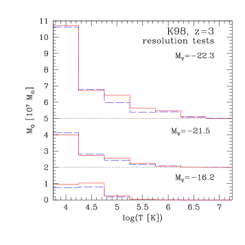
Figure 16: Gas-phase oxygen temperature distributions for three proto-galactic regions simulated at both very high (blue dashed histograms) and normal (red solid histograms) numerical resolution. The three proto-galaxies become at $z$=0 disc galaxies of characteristic circular velocities $V_{c}$=245, 180 and 66 km/s, respectively. The oxygen masses for the smaller galaxy have been multiplied by a factor 50 for clarity. The slight offset between the results for the smaller galaxy is due to high resolution proto-galactic region being slightly smaller than the corresponding normal resolution one.

In SGP03 and Sommer-Larsen (2006) it has been shown that the results of cosmological galaxy formation and evolution using our code are, in general, robust to changes of the numerical resolution. However, in this paper we present gas-phase metal temperature distributions and other results, which have not been presented before. It is hence clearly important to demonstrate that these results are resolution robust as well. To this end we carried out three very high resolution K98 IMF simulations, of eight times higher mass and two times higher force resolution compared to “standard”. We simulated three (proto-)disc galaxies, which at $z$=0 have characteristic circular velocities of 245, 180 and 66 km/s. The galaxy forming regions were represented by a total of about 2.2, 1.2 and 1.3 million particles, compared to the about 290 000, 150 000 and 210 000 particles used at “normal” resolution (for computational reasons the region simulated at very high resolution for the last galaxy was slightly smaller than the corresponding “normal” resolution one). Gas and star particle masses were $m_{\rm{gas}}$=$m_{*}$=9.1$\times$10⁴ and 2.5$\times$10³ $h^{-1}$M_⊙ for the first two galaxies and the last one, respectively. The corresponding dark matter particle masses were $m_{\rm{DM}}$=5.2$\times$10⁵ and 1.4$\times$10⁴ $h^{-1}$M_⊙. Moreover, gravitational (spline) softening lengths of $\epsilon_{\rm{gas}}$=$\epsilon_{*}$=190 and $\epsilon_{\rm{DM}}$=340 $h^{-1}$pc, respectively, were adopted for the first two galaxies, and 57 and 100 $h^{-1}$pc for the latter. Other results for the first two runs have already been presented in Sommer-Larsen (2006), Razoumov & Sommer-Larsen (2006), Greve & Sommer-Larsen (2007), Laursen & Sommer-Larsen (2007) and Ellison et al. (2007).

In Fig. 16 is shown the gas-phase oxygen temperature distributions for the three very high resolution runs, together with the results of the normal resolution ones — note that the oxygen masses for the smaller galaxy have been multiplied by a factor 50 for clarity. It is seen that the general agreement is very good; the slight disagreement for the small galaxy is due to the fact that the region simulated at very high resolution was slightly smaller than the corresponding normal resolution one.

Due to computational limitations we did not perform similar resolution tests for the two other IMFs considered, but we have no reason to believe that simulations based on these IMFs would perform less well in resolution tests. We conclude that the results obtained in this paper are robust to resolution changes.

10 Summary and conclusions

The global temperature distribution of the cosmic gas-phase oxygen at $z$$\sim$3 has been determined by combining high resolution cosmological simulations of individual proto-galactic, as well as larger, regions with extinction-corrected, observationally based, V-band (rest-frame) galaxy luminosity functions (LFs) of faint end slopes $\alpha=-1.85$ and $-1.57$. The simulations have been performed with three different stellar initial mass functions (IMFs), a Kroupa (K98), a Salpeter (S) and an Arimoto-Yoshii (AY), spanning a range of a factor of five in chemical yield and specific SNII energy feedback. Gas-phase oxygen is binned according to $T$ as log$(T)\la 4.0$ (“cold”), log$(T)\sim 4.5$ (“warm”), and log$(T)\sim$5.0, 5.5, 6.0, 6.5, 7.0 (“hot” phases). Below we summarize results for the $\alpha=-1.85$ LF, but results for the $\alpha=-1.57$ LF are similar.

Oxygen is found to be distributed over all $T$ phases, in particular for the (“top-heavy”) AY IMF. But, at variance with previous works, it is found that, for the K98 and Salpeter IMFs, the most important phase is the cold one, which contains 47 and 37% of all gas-phase oxygen, mainly in gas at fairly high density, $n_{\rm{H}}$$\ga$0.1 cm^-3, and potentially star-forming. Moreover, the cold phase alone contains 1.3, 1.5 and 3.2 times the mass of oxygen in galactic stars for the three IMFs. The implications of this in relation to observational damped Lyman-$\alpha$ absorber (DLA) studies are discussed on the basis of very-high resolution simulations of two (proto-)disc galaxies, with emphasis on oxygen and iron abundances. It is concluded, that the reason why current DLA surveys only detect a cold ISM metal fraction of about 20% relative to the metal mass in galactic stars is that the total cross-section for the high-metallicity component is only of order a few percent of the total DLA cross-section, and that the current DLA samlpes are too small to uncover it. Moreover, in addition, dust bias, as well as H₂ formation, will likely also be of importance.

In relation to “missing metals” it is found that the ratio of gas-phase to stellar oxygen mass is 2.7, 3.9 and 13, and the ratio of warm+hot to cold gas-phase oxygen mass is 1.1, 1.7 and 3.2 for the three IMFs. For the AY IMF, the hot phases actually contain more oxygen than the cold+warm.

In conclusion, a significant fraction of the cosmic oxygen may be difficult or impossible to detect. In addition, it is found that less than about 20-30% of the cosmic oxygen will be associated with galaxies brighter than $M_{\rm{V}}\sim-22$, i.e., the faintest galaxy luminosities probed by current LBG metallicity determinations (about one mag. below $L^{*}$). Hence, 70-80% of the cosmic oxygen is also in this sense “missing”.

From the LBG based, $\lambda$$\sim$1500 Å UV luminosity density history at $z$$\geq$3, we obtain an essentially IMF independent constraint on the mean cosmic oxygen density at $z$=3. We compare this to what is obtained from our models, for the three different IMFs. We find that the (solar neighbourhood type) K98 IMF is strongly excluded, as the chemical yield is simply too small, the Salpeter is marginally excluded, and the AY matches the constraint well. The optimal IMF would have a yield intermediate between the S and AY. The K98 IMF can only match the data if the $\lambda$$\sim$1500 Å extinction corrections have been overestimated by factor of $\sim$4, which seems highly unlikely, cf. Reddy & Steidel (2004).

Using carbon abundances, and C to C iv ionisation corrections, we estimate $\Omega$(C iv) at moderate IGM gas over-densities, $\delta=\rho_{\rm{gas}}/\bar{\rho}_{\rm{gas}}\sim 1-100$ for the three IMFs, and compare to observational results. As above, we find that the yield of the K98 IMF is too small to match the data, whereas models based on the Salpeter and AY IMFs can match the data, with the optimal IMF in between the two. Moreover, we show that for all IMFs, C iv abundance weighted IGM temperatures are moderate, $T$$\la$4$\times$10⁴ K, consistent with observational constraints on C iv line widths.

References

- [1] Adelberger, K.L., Steidel, C.C., 2000, ApJ, 544, 218
- [2] Adelberger, K.L., et al. , 2003, ApJ, 584, 45
- [\citeauthoryearAdelberger, Steidel, Shapley, Hunt, Erb, Reddy & PettiniAdelberger et al.2004] Adelberger K. L., Steidel C. C., Shapley A. E., Hunt M. P., Erb D. K., Reddy N. A., Pettini M., 2004, ApJ, 607, 226
- [\citeauthoryearAdelberger et al. 2005] Adelberger K. L., Shapley A. E., Steidel C. C., Pettini M., Erb D. K., & Reddy N. A. 2005, A pJ, 629, 636
- [3] Akerman, C. J., et al., 2005, A&A, 440, 499
- [4] Aracil, B., Petitjean, P., Pichon, C. & Bergeron, J. 2004, A&A, 419, 811
- [5] Arimoto, N., & Yoshii, Y. 1987, A&A, 173, 23
- [6] Baldry, I.K., et al. , 2005, MNRAS, 358, 441
- [Barger et al. (1998)] Barger, A.J., et al. 1998, Nature, 394, 248
- [7] Bergeron, J., Aracil, B., Petitjean, P. & Pichon, C. 2002, A&A, 396, L11
- [8] Bergeron, J. & Herbert-Fort, S. 2005, astro-ph/0506700
- [\citeauthoryearBlain, Chapman, Smail & IvisonBlain et al.2004] Blain A. W., Chapman S. C., Smail I., Ivison R., 2004, ApJ, 611,
- [9] Bloom, J.S., Kulkarni, S.R., Djorgovski, S.G., 2002, AJ, 123, 1111
- [10] Boissier,S., & Prantzos, N. 1999, MNRAS, 307, 857
- [\citeauthoryearBokensberg, Sargent, & Rauch 2003] Boksenberg, A., Sargent, W. L. W., & Rauch, M. 2003, ASP Conference Proceedings, Vol. 297, 447, eds. Edited E. Perez, R.M.G. Delgado, & G. Tenorio-Tagle
- [Bouché, Lehnert & Péroux (2006a)] Bouché, N., Lehnert, M . D., Péroux, C. 2006a, MNRAS, 364, 319
- [Bouché, Lehnert & Péroux (2006b)] Bouché, N., Lehnert, M . D., Péroux, C. 2006b, MNRAS, 367, L16
- [11] Bouché, N., Lehnert, M. D., Aguirre, A., Péroux, C., Bergeron, J., 2007, MNRAS, in press (astro-ph/0703509)
- [Bouwens et al.(2004)] Bouwens, R. J., et al. 2004a, ApJL, 606, L25
- [Bouwens et al. 2004] Bouwens, R. J., et al. 2004b, ApJL, 616, L79
- [Bouwens et al. 2006] Bouwens, R. J., Illingworth, G.D., Blakeslee, J.P., & Franx, M., 2006, ApJ, 653, 53
- [Bouwens et al. 2007] Bouwens, R. J., Illingworth, G.D., Franx, M., & Ford, H. 2007, ApJ, in press (astroph/0707.2080)
- [\citeauthoryearBryan et al.1998] Bryan G.L., Norman M.L., 1998, ApJ 495, 80
- [Bunker, Stanway, Ellis, & McMahon(2004)] Bunker, A. J., Stanway, E. R., Ellis, R. S., & McMahon, R. G. 2004, MNRAS, 355, 374
- [Calura & Matteucci (2004)] Calura, F. & Matteucci, F. 2004, MN RAS, 351, 384
- [Calura & Matteucci (2006)] Calura, F. & Matteucci, F. 2006, MN RAS, 369, 465
- [12] Carswell, B., Schaye, J. & Kim, T.-S. 2002, ApJ, 578, 43
- [Chapman et al. (2005)] Chapman, S.C., Blain, A.W., Smail, I., & Ivison, R.J. 2005, ApJ, 622, 772
- [\citeauthoryearCole et al. 2001] Cole, S., et al. 2001, MNRAS, 326, 255
- [13] Conselice C.J., Bundy K.E., Richard S., Brichmann J., Vogt N.P., Phillips A.C., 2005, ApJ 628, 160
- [\citeauthoryearCroft et al. 1998] Croft, R. A. C., W einberg, D. H., Katz, N., & Herquist, L. 1998, ApJ, 495, 44
- [14] Dahlen, T., Mobasher, B., Dickinson, M., Ferguson, H.C., Giavalisco, M., Kretchmer, C., Ravindranath, S., 2007, ApJ, 654, 172
- [15] D’Antona, F., & Caloi, V., 2004, ApJ, 611, 871
- [16] Davé, R., & Oppenheimer, B., 2006, MNRAS, (DO06)
- [Eales et al. (1999)] Eales, S., et al. 1999, ApJ, 515, 518
- [] Ellingson E., Lin H., Yee H.K.C., Carlberg R.G., 2001, ApJ 547, 609
- [] Ellison, S.L., et al., 2001, A&A, 379, 393
- [] Ellison, S.L., et al., 2004, ApJ, 615, 118
- [] Ellison, S.L., Hall, B. H., & Lira, P., 2005, AJ, 130, 1345
- [] Ellison, S.L., Hennawi, J.F., Martin, C.L., Sommer-Larsen, J., 2007, MNRAS, submitted
- [] Elmegreen, B., 2006, ApJ, 648, 572
- [] Erni, P., et al., 2006, A&A, 354, 19
- [] Ferland, G.J., Korista, K.T., Verner, D.A., Ferguson, J.W., Kingdon, J.B., Verner, E.M., 1998, PASP, 110, 761
- [] Ferrara, A., Scannapieco, E., Bergeron, J. 2005, ApJL, 634, L37 (FSB05)
- [] Fox, A.J. et al. , 2007, A&A, in press (astro-ph/0701392)
- [\citeauthoryearFranx, Labbé, Rudnick, van Dokkum, Daddi, Förster Schreiber, Moorwood, Rix, Röttgering, van de Wel, van der Werf & van StarkenburgFranx et al.2003] Franx M., Labbé I., Rudnick G., van Dokkum P. G., Daddi E., Förster Schreiber N. M., Moorwood A., Rix H., Röttgering H., van de Wel A., van der Werf P., van Starkenburg L., 2003, ApJ, 587, L79
- [17] Fruchter, A.S. et al. , 2006, Nature, 441, 463
- [] Fynbo, J.P.U. et al. , 1999, MNRAS, 305, 849
- [] Fynbo, J.P.U. et al. , 2001, A&A, 374, 443
- [] Fynbo, J.P.U. et al. , 2003, A&A, 407, 147
- [] Fynbo, J.P.U. et al. , 2006, A&AL, 451, L47
- [] Gawiser, E. et al. , 2006, ApJL, 642, L13
- [Giavalisco et al.(2004)] Giavalisco, M., et al. 2004, ApJL, 600, L103
- [\citeauthoryearGreve, Bertoldi, Smail, Neri, Chapman, Blain, Ivison, Genzel, Omont, Cox, Tacconi & KneibGreve et al.2005] Greve T. R., Bertoldi F., Smail I., Neri R., Chapman S. C., Blain A. W., Ivison R. J., Genzel R., Omont A., Cox P., Tacconi L., Kneib J. ., 2005, MNRAS, 359, 1165
- [] Greve, T.R., Sommer-Larsen, J., 2007, ApJ, submitted (astro-ph/0608683)
- [\citeauthoryearHaardt & Madau 1996] Haardt, F. & Madau, P. 1996, ApJ, 461, 20
- [\citeauthoryearHaardt & Madau 2001] Haardt, F. & Madau, P. 2001, in “Clusters of galaxies and the high redshift universe observed in X-rays, Recent results of XMM-Newton and Chandra”, XXXVIth Rencontres de Mor iond , eds. D.M. Neumann & J.T.T. Van
- [] Haehnelt et al. 2000, ApJ, 534, 594
- [] Herbert-Fort, S., et al. , 2006, PASP, 118, 1077
- [18] Jakobsson, P., et al. 2005, MNRAS, 362, 245
- [19] Jakobsson, P., et al. 2006, A&AL, 460, L13
- [20] Johansson, P., Efstathiou, G., 2006, MNRAS, 371, 1519
- [21] Jorgenson, R., A. et al. 2006, ApJ, 646, 730
- [22] Kennicutt R.C., 1998, ApJ, 498, 541
- [23] Kroupa P., 1998, MNRAS, 298, 231
- [24] Lacey, C. G., Baugh, C. M., Frenk, C. S., Granato, G. L., Silva, L., Bressan, A., Cole, S., 2005, in the proceedings of the conference ”The fabulous destiny of galaxies: bridging past and present”, 20-24 June 2005, (astro-ph/0509715))
- [25] Larsson, J., et al. , 2007, MNRAS, in press (astro-ph/0701562)
- [26] Laursen, P., Sommer-Larsen, J., 2007, ApJL, 657, L59
- [27] Ledoux, C., et al. , 2002, A&A, 392, 781
- [28] Ledoux, C., et al. , 2003, MNRAS, 346, 209
- [Lia et al.(2002a)] Lia, C., Portinari, L., Carraro, G. 2002a, MNRAS, 330, 821
- [Lia et al.(2002b)] Lia, C., Portinari, L., Carraro, G. 2002b, MNRAS, 335, 864
- [29] Loewenstein, M., 2006, ApJ, 648, L230
- [30] Lu, L., et al. , 1996, ApJS, 104, 475
- [31] Lucatello, S., Gratton, R.G., Beers, T.C., & Carretta, E., 2005, ApJ 625, 833
- [32] Kulkarni, V. P., & Fall, S. M., 2002, ApJ, 580, 732
- [33] Madau, P., et al. 1996, MNRAS, 283, 1388
- [34] Madau, P., Pozzetti, L., & Dickinson, M., 1998, ApJ, 498, 106
- [35] Milne, M.L., Pritchet, C.J., Poole, G.B., Gwyn, S.D.J., 2007, AJ, 133, 177
- [36] Møller, P., et al. , 2002, ApJ, 574, 51
- [37] Murphy, M.T., & Liske, J., 2004, MNRAS, 354, L31
- [] Nilsson, K., et al. , 2007, A&A, submitted
- [38] Norberg, P. et al. , 2002, MNRAS, 336, 907
- [39] Oppenheimer, B., & Davé, R., 2006, MNRAS, (OD06)
- [40] Pagel, B.E.J., 1999, in ASP Conf. Series The Low Surface Brightness Universe, ed. J.J.Davies, C.Impey, & S.Phillipps (San Francisco:ASP), vol.170, p.375
- [41] Pei, Y.C., Fall, S.M. & Bechtold, J., 1991, ApJ, 378, 6
- [Pelupessy, Papadopoulos & van der Werf (2006)] Pelupessy, I., Papadopoulos, P. P. & van der Wer, P. 2006, ApJ, 645, 1024.
- [42] Petitjean, P. & Bergeron, J., 1994, A&A, 283, 759
- [43] Petitjean, P. et al. , 2006, A&AL, 456, L9
- [44] Pettini, M., et al. , 1990, ApJ, 348, 48
- [45] Pettini, M., et al. , 1994, ApJ, 426, 78
- [46] Pettini, M. ESO Workshop, Chemical Evolution from Zero to High Redshift, 233-247 (1999)
- [Pettini et al. (2001)] Pettini, M., Shapley, A. E., Steidel, C. C., Cuby, J.-G., Dickinson, M., Moorwood, A. F. M., Adelberger, K. L., Giavalis co, M. 2001, ApJ, 554, 981
- [\citeauthoryearPettini, Madau, Bolte, Prochaska, Ellison & FanPettini et al.2003] Pettini M., Madau P., Bolte M., Prochaska J. X., Ellison S. L., Fan X., 2003, ApJ, 594, 695
- [Pettini (2004)] Pettini, M. 2004, in proc. “Cosmochemistry. The melting pot of the elements”, eds. C. Esteban, R. J. Garcí López, A. Herrer o, F. Sánchez, Cambridge, UK: Cambridge University Press, p.257
- [47] Porciani, C., Madau, P., 2005, ApJ, 625, L43
- [48] Portinari, L., Moretti, A., Chiosi, C., & Sommer-Larsen, J., 2004, ApJ, 604,579
- [49] Portinari, L., Sommer–Larsen, J., 2007, MNRAS, 375, 913
- [50] Prantzos, N., & Charbonnel, C., 2006, A&A, 458, 135
- [51] Prochaska, J. X., Gawiser, E., Wolfe, A. M., Castro, S. & Djorgovski, S. G. 2003, ApJL, 595, L9
- [52] Prochaska, J. X., Herbert-Fort, S., Wolfe, A. M., 2005, ApJ, 635, 123
- [Prochaska et al. (2006)] Prochaska, J. X., O’Meara, J. M., Herbert-Fort, S., Burles, S., Prochter, G. E., Bernstein, R. A. 2006, ApJL, 648, L97
- [Prochaska et al. (2007)] Prochaska, J. X., et al., 2007, ApJ, submitted (astro-ph/0703665)
- [\citeauthoryearRauch et al. 2005] Rauch, M., Becker, G. D., Viel, M., Sargent, W. L. W., Smette, A., Simcoe, R. A., Barlow, T. A., H
- [53] Razoumov, A.O., Sommer-Larsen, J., 2006, ApJL, 651, L89
- [54] Razoumov, A.O., Sommer-Larsen, J., 2007, ApJ, submitted (astro-ph/0702321)
- [55] Reddy, N. A. & Steidel, C. C. 2004, ApJ, 603, L13
- [Reddy et al. (2005)] Reddy, N.A., Erb, D.K., Steidel, C.C., Shapley, A.E., Adelberger, K.L., & Pettini, M. 2005, ApJ, 633, 748
- [56] Richards, G.T., et al. , 2006, AJ, 131, 2766
- [Robertson et al. (2004)] Robertson, B., Yoshida, N., Springel, V., & Hernquist, L. 2004, ApJ, 606, 32
- [57] Romeo, A.D., Sommer–Larsen, J., Portinari, L., Antonuccio–Delogu, V., 2006, MNRAS, 371, 548
- [Schiminovich et al.(2005)] Schiminovich, D., et al. 2005, ApJL, 619, L47
- [58] Salpeter E.E., 1955, ApJ 121, 161
- [59] Savaglio, S., 2006, NJPh, 8, 195
- [60] Sawicki, M., Thompson, D., 2006, ApJ 648, 299
- [61] Scannapieco, E., 2005, ApJ, 624, L1
- [62] Scannapieco, E. et al., 2006, MNRAS.365, 615
- [63] Schaye, J., Rauch, M., Sargent, W.L.W., Kim, T., 2000, ApJL, 541, L1
- [64] Schaye, J., 2001, ApJL, 559, L1
- [65] Schaye, J., 2001b, ApJL, 562, L95
- [\citeauthoryearSchaye et al. 2003] Schaye, J., Aguirre, A., Kim, T.-S., Theuns, T., Rauch, M., & Sargent, W.L.W. 2003, ApJ, 596, 768
- [66] Serjeant, S., & Harrison, D., 2005, MNRAS, 356, 192
- [67] Simcoe, R. A., Sargent, W. L. W. & Rauch, M. 2004, ApJ, 606, 92
- [\citeauthoryearShapley et al. 2001] Shapley, A. E., Steidel, C. C., Adelberger, K. L., Dickinson, M., Giavalisco, M., & Pettini, M. 2001, ApJ, 562, 95
- [\citeauthoryearShapley et al. 2003] Shapley, A. E., Steidel, C. C., Pettini, M., & Adelberger, K. L. 2003, ApJ, 588, 65
- [Smail et al. (1997)] Smail, I., Ivison, R.J., & Blain, A.W. 1997, ApJ, 490, L5
- [\citeauthoryearSpringel & Hernquist 2002] Springel, V. & Hernquist, L. 2002, MNRAS, 333, 649
- [\citeauthoryearSpringel & Hernquist 2003] Springe l, V. & Hernquist, L. 2003, MNRAS, 339, 289
- [68] Sommer–Larsen, J., 2006, ApJ, 644, L1
- [69] Sommer–Larsen, J., Gelato S., Vedel, H., 1999, ApJ 519, 501
- [70] Sommer–Larsen, J., Götz M., Portinari L., 2003, ApJ 596, 47 (SGP03)
- [71] Sommer–Larsen, J., & Fynbo, J., 2007, MNRAS, to be submitted
- [] Sommer-Larsen, J., Razoumov, A.O., Ellison, S.L., Hennawi, J.F., Martin, C.L., 2007, MNRAS, to be submitted
- [72] Songaila, A., Cowie, L.L., Lilly, S.J., 1990, ApJ, 348, 371
- [\citeauthoryearSongaila 2001] Songaila, A. 2001, ApJ , 561, L153
- [\citeauthoryearSongaila 2005] Songaila, A. 2005, AJ, 130, 1996
- [Steidel et al. (1999)] Steidel, C. C., Adelberger, K. L., Giavalisco, M., Dickinson, M. and Pettini, M. 1999, ApJ, 519, 1
- [\citeauthoryearSutherland & Dopita 1993] Sutherland , R. S. & Dopita, M. A. 1993, ApJS, 88, 253
- [Tripp et al. (2006)] Tripp, T. M., Bowen, D. V., Sembach, K. R., Jenkins, E. B., Savage, B. D., Richter, P. 2006, in “Astrophysics in the Far Ultraviolet: Five Years of Discovery with FUSE”, eds. G. Sonneborn and H. Moos
- [73] Thacker, R.J., Couchman, H.M.P., 2001, ApJ, 555, L17
- [74] Turnshek et al. 1989, ApJ, 344, 567
- [\citeauthoryearvan Dokkum et al.van Dokkum et al.2 003] van Dokkum P. G. et al., 2003, ApJ, 587, L83
- [75] Vladilo, G., & Péroux, C., 2005, A&A, 444, 461
- [76] Vladilo, G., Centurión, M., Levshakov, S.A., Péroux, C., Khare, P., Kulkarni, V.P., York, D.G., 2006, A&A, 454, 151
- [77] Weidner, C., & Kroupa, P., 2006, MNRAS, 365, 1333
- [78] Wolfe, C. A., Gawiser, E. & Prochaska, J. X. 2003, ApJ, 593, 235
- [79] Yamanoi, H., et al. 2007, AJ, submitted (astro-ph/0701670)
- [80] Zwaan, M., et al., 2005, MNRAS, 364, 1467
- [81] Zwaan, M., & Prochaska, J. X., 2006, ApJ, 643, 675