Detecting ionized bubbles in redshifted 21 cm maps

Abstract

The reionization of the Universe, it is believed, occurred by the growth of ionized regions (bubbles) in the neutral intergalactic medium (IGM). We study the possibility of detecting these bubbles in radio-interferometric observations of redshifted neutral hydrogen (HI) $21$ cm radiation. The signal $(<1\,{\rm mJy})$ will be buried in noise and foregrounds, the latter being at least a few orders of magnitude stronger than the signal. We develop a visibility based formalism that uses a filter to optimally combine the entire signal from a bubble while minimizing the noise and foreground contributions. This formalism makes definite predictions on the ability to detect an ionized bubble or conclusively rule out its presence in a radio-interferometric observation. We make predictions for the currently functioning GMRT and a forthcoming instrument, the MWA at a frequency of 150 MHz (corresponding to a redshift of 8.5). For both instruments, we show that a $3\,\sigma$ detection will be possible for a bubble of comoving radius $R_{b}\geq 40\,{\rm Mpc}$ (assuming it to be spherical) in $100\,{\rm hrs}$ of observation and $R_{b}\geq 22\,{\rm Mpc}$ in $1000\,{\rm hrs}$ of observation, provided the bubble is at the center of the field of view. In both these cases the filter effectively removes the expected foreground contribution so that it is below the signal, and the system noise is the deciding criteria. We find that there is a fundamental limitation on the smallest bubble that can be detected arising from the statistical fluctuations in the HI distribution. Assuming that the HI traces the dark matter we find that it will not be possible to detect bubbles with $R_{b}<8\,{\rm Mpc}$ using the GMRT and $R_{b}<16\,{\rm Mpc}$ using the MWA, however large be the integration time.

1 Introduction

Quasar absorption spectra (Becker et al., 2001; Fan et al., 2002) and CMBR observations (Spergel et al., 2006; Page et al., 2006) together imply that reionization occurred over an extended period spanning the redshift range $6\leq z\leq 15$ (for reviews see Fan, Carilli & Keating 2006; Choudhury & Ferrara 2006a). It is currently believed that ionized bubbles produced by the first luminous objects grow and finally overlap to completely reionize the universe (Barkana & Loeb, 2001; Furlanetto, Zaldarriaga & Hernquist, 2004). In this paper we consider the possibility of detecting these ionized bubbles in redshifted $21\,{\rm cm}$ neutral hydrogen (HI) maps.

An ionized bubble embedded in neutral hydrogen will appear as a decrement in the background redshifted 21 cm radiation. This decrement will typically span across several pixels and frequency channels in redshifted 21 cm maps. Detecting this is a big challenge because the HI signal ($\sim 1\,{\rm mJy}$ or lower ) will be buried in foregrounds (Shaver et al., 1999; DiMatteo. et al., 2002; Oh, 1999; Cooray & Furlanetto, 2004; Santos, Cooray & Knox, 2005) which are expected to be at least $2-3$ orders of magnitude larger. An objective detection criteria which optimally combines the entire signal in the bubble while minimizing contributions from foregrounds, system noise and other such sources is needed to search for ionized bubbles. The noise in different pixels of maps obtained from radio-interferometric observations is correlated (eg. Thompson, Moran & Swenson (1986)), and it is most convenient to deal with visibilities instead. These are the primary quantities that are measured in radio-interferometry. In this paper we develop a visibility based formalism to detect an ionized bubble or conclusively rule it out in radio-interferometric observations of HI at high redshifts.

The paper is motivated by the fact that the Giant Metre-Wave Radio Telescope (GMRT; Swarup et al. 1991) which is currently functional has a band centered around $150\,{\rm MHz}$ which corresponds to HI at $z\sim 8.5$. There are several low frequency radio telescopes which are expected to become functional in the future (eg. MWA, LOFAR, 21 CMA and SKA) all of which are being designed to be sensitive to the epoch of reionization HI signal. In this paper we apply our formalism for detecting ionized bubbles to make predictions for the GMRT and for one of the forthcoming instruments, namely the MWA. For both telescopes we investigate the feasibility of detecting the bubbles, and in situations where a detection is feasible we predict the required observation time. For both telescopes we make predictions for observations only at a single frequency ($150{\rm MHz}$), the aim here being to demonstrate the utility of our formalism and not present an exhaustive analysis of the feasibility of detecting ionized bubbles in different scenarios and circumstances. For the GMRT we have used the telescope parameters from their website, while for the MWA we use the telescope parameters from Bowman et al. (2006). It may be noted that MWA is expected to be gradually expanded in phases, and we have used the parameters corresponding to an early stage, the MWA - Low Frequency Demonstrator.

It is expected that detection of individual bubbles would complement the studies of reionization through the global statistical signal of the redshifted $21\,{\rm cm}$ radiation which has been studied extensively (eg. Zaldarriaga, Furlanetto & Hernquist 2004; Morales & Hewitt 2004; Bharadwaj & Ali 2005; Bharadwaj & Pandey 2005; for a recent review see Furlanetto et al. 2006).

The outline of the paper is as follows: In Section 2 we discuss various sources which are expected to contribute in low frequency radio-interferometric observation, this includes the signal expected from an ionized bubble. In Section 3 we present the formalism for detecting an ionized bubble, and in Section 4 we present the results and discuss its implications. The cosmological parameters used throughout this paper are those determined as the best-fit values by WMAP 3-year data release, i.e., $\Omega_{m}=0.23,\Omega_{b}h^{2}=0.022,n_{s}=0.96,h=0.74,\sigma_{8}=0.76$ (Spergel et al. 2006).

2 Different sources that contribute to low frequency radio observations

The quantity measured in radio-interferometric observations is the visibility $V({\vec{U}},\nu)$ which is measured in a number of frequency channels $\nu$ across a frequency bandwidth $B$ for every pair of antennas in the array. For an antenna pair, it is convenient to use ${\vec{U}}={\vec{d}}/\lambda$ to quantify the antenna separation ${\vec{d}}$ projected in the plane perpendicular to the line of sight in units of the observing wavelength $\lambda$. We refer to ${\vec{U}}$ as a baseline. The visibility is related to the specific intensity pattern on the sky $I_{\nu}(\vec{\theta})$ as

$$V({\vec{U}},\nu)=\int d^{2}\theta A(\vec{\theta})I_{\nu}(\vec{\theta})e^{2\pi\imath\vec{\theta}\cdot{\vec{U}}}$$ (1)

where $\vec{\theta}$ is a two dimensional vector in the plane of the sky with origin at the center of the field of view, and $A(\vec{\theta})$ is the beam pattern of the individual antenna. For the GMRT this can be well approximated by Gaussian $A(\vec{\theta})=e^{-{\theta}^{2}/{\theta_{0}}^{2}}$ where $\theta_{0}\approx 0.6~{}\theta_{\rm FWHM}$ and we use the values $2.28\degr$ for $\theta_{0}$ at $153\,{\rm MHz}$ for the GMRT. Each MWA antenna element consists of $16$ crossed dipoles distributed uniformly in a square shaped tile, and this is stationary with respect to the earth. The MWA beam pattern is quite complicated, and it depends on the pointing angle relative to the zenith (Bowman et al., 2007). Our analysis largely deals with the beam pattern within $1^{\circ}$ of the pointing angle where it is reasonable to approximate the beam as being circularly symmetric (Figures 3 and 5 of Bowman et al. 2007 ). We approximate the MWA antenna beam pattern as a Gaussian with $\theta_{0}=18\degr$ at $153\,{\rm MHz}$. Note that the MWA primary beam pattern is better modeled as $A(\vec{\theta})\propto\cos^{2}(K\theta)$, but a Gaussian gives a reasonable approximation in the center of the beam which is the region of interest here. Equation (1) is valid only under the assumption that the field of view is small so that it can be well approximated by a plane, or under the unlikely circumstances that all the antennas are coplanar.

The visibility recorded in $150\,{\rm MHz}$ radio-interferometric observations is a combination of three separate contributions

$$V(\vec{U},\nu)=S(\vec{U},\nu)+N(\vec{U},\nu)+F(\vec{U},\nu)$$ (2)

where $S(\vec{U},\nu)$ is the HI signal that we are interested in, $N(\vec{U},\nu)$ is the system noise which is inherent to the measurement and $F(\vec{U},\nu)$ is the contribution from other astrophysical sources referred to as the foregrounds. Man-made radio frequency interference (RFI) from cell phones and other communication devices are also expected to contribute to the measured visibilities. Given the lack of a detailed model for the RFI contribution, and anticipating that it may be possible to remove it before the analysis, we do not take it into account here.

2.1 The HI signal from ionized bubbles

According to models of reionization by UV sources, the early stages of reionization are characterized by ionized HII regions around individual source (QSOs or galaxies). As a first approximation, we consider these regions as ionized spherical bubbles characterized by three parameters, namely, its comoving radius $R_{b}$, the redshift of its center $z_{c}$ and the position of the center determined by the two-dimensional vector in the sky-plane $\vec{\theta}_{c}$. The bubble is assumed to be embedded in an uniform intergalactic medium (IGM) with a neutral hydrogen fraction $x_{\rm HI}$. We use $r_{\nu}$ to denote the comoving distance to the redshift where the HI emission, received at a frequency $\nu=1420\,{\rm MHz}/(1+z)$, originated, and define $r^{\prime}_{\nu}=d\,r_{\nu}/d\,\nu$. The planar section through the bubble at a comoving distance $r_{\nu}$ is a disk of comoving radius $R_{\nu}=R_{b}\sqrt{1-(\Delta\nu/\Delta\nu_{b})^{2}}$ where $\Delta\nu=\nu_{c}-\nu$ is the distance from the the bubble center $\nu_{c}$ in frequency space with $\nu_{c}=1420\,{\rm MHz}/(1+z_{c})$ and $\Delta\nu_{b}=R_{b}/r^{\prime}_{\nu_{c}}$ is the bubble size in the frequency space. The bubble, obviously, extends from $\nu_{c}-\Delta\nu_{b}$ to $\nu_{c}+\Delta\nu_{b}$ in frequency and in each frequency channel within this frequency range the image of the ionized bubble is a circular disk of angular radius $\theta_{\nu}=R_{\nu}/r_{\nu}$; the bubble is not seen in HI beyond this frequency range. Under such assumptions, the specific intensity of the redshifted HI emission is

$$I_{\nu}(\vec{\theta})=\bar{I}_{\nu}x_{\rm HI}\left[1-\Theta\left(1-\frac{\mid\vec{\theta}-\vec{\theta}_{c}\mid}{\theta_{\nu}}\right)\right]\Theta\left(1-\frac{\mid\nu-\nu_{c}\mid}{\Delta\nu_{b}}\right)$$ (3)

where $\bar{I_{\nu}}=2.5\times 10^{2}\frac{Jy}{sr}\left(\frac{\Omega_{b}h^{2}}{0.02}\right)\left(\frac{0.7}{h}\right)\left(\frac{H_{0}}{H(z)}\right)$ is the radiation background from the uniform HI distribution and $\Theta(x)$ is the Heaviside step function.

The soft X-ray emission from the quasar responsible for the ionized region is expected to heat the neutral IGM in a shell around the ionized bubble. The HI emission from this shell is expected to be somewhat higher than $\bar{I}_{\nu}$ (Wyithe & Loeb, 2004). We do not expect this to make a very big contribution, and we do not consider this here.

If we assume that the angular extent of the ionized bubble is small compared to the angular scale of primary beam ie. $\theta_{\nu}\ll\theta_{0}$, we can take $A(\vec{\theta})$ outside the integral in eq. (1) and write the signal as $A(\vec{\theta}_{c})\int d^{2}\theta I_{\nu}(\vec{\theta})e^{2\pi\imath\vec{\theta}\cdot{\vec{U}}}$, which essentially involves a Fourier transform of the circular aperture $\Theta\left(1-\mid\vec{\theta}-\vec{\theta}_{c}\mid r_{\nu}/R_{\nu}\right)$. For example, a bubble of radius as large as 40 Mpc at $z=8.5$ would have an angular size of only $\theta_{\nu}\approx 0.25^{\degr}$ which satisfies the condition $\theta_{\nu}\ll\theta_{0}$. In a situation where the bubble is at the center of the field of view, the visibility is found to be

$$S_{\rm center}({\vec{U}},\nu)=-\pi\bar{I_{\nu}}x_{\rm HI}\theta^{2}_{\nu}\left[\frac{2J_{1}(2\pi U\theta_{\nu})}{2\pi U\theta_{\nu}}\right]\Theta\left(1-\frac{\mid\nu-\nu_{c}\mid}{\Delta\nu_{b}}\right)$$ (4)

where $J_{1}(x)$ is the first order Bessel function. Note that $S_{\rm center}({\vec{U}},\nu)$ is real and it is the Fourier transform of a circular aperture. The uniform HI background also contributes $\bar{I_{\nu}}\pi\theta_{0}^{2}{\rm e}^{-\pi^{2}\theta_{0}^{2}U^{2}}$ to the visibility, but this has been dropped as it is quite insignificant at the baselines of interest. Note that the approximations used in eqs. (4) have been tested extensively by comparing the values with the numerical evaluation of the integral in eq. (1). We find that the two match to a high level of accuracy for the situations of interest here. In the general situation where the bubble is shifted by $\vec{\theta}_{c}$ from the center of the field of view, the visibility is given by

$$S({\vec{U}},\nu)={\rm e}^{-\theta_{c}^{2}/\theta_{0}^{2}}e^{2\pi i{\vec{U}}\cdot\vec{\theta}_{c}}S_{\rm center}({\vec{U}},\nu)$$ (5)

i.e., there is a phase shift of ${\rm e}^{2\pi i{\vec{U}}\cdot\vec{\theta}_{c}}$ and a ${\rm e}^{-\theta_{c}^{2}/\theta_{0}^{2}}$ drop in the overall amplitude.

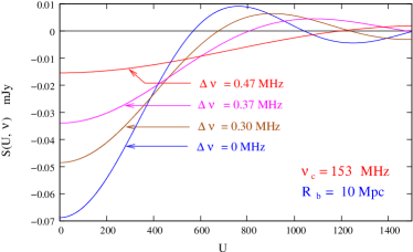
Figure 1: Signal from a spherical ionized bubble of comoving radius $10\,{\rm Mpc}$ as a function of baseline $U$ for different frequency channels.

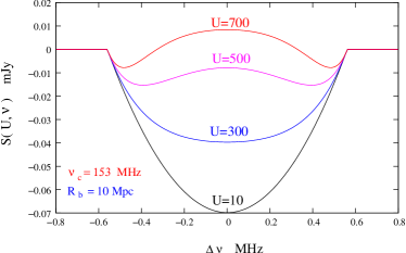
Figure 2: Signal from a spherical ionized bubble of comoving radius $10\,{\rm Mpc}$ as a function of $\Delta\nu=\nu-\nu_{c}$ for different baselines.

Figures 1 and 2 show the $U$ and $\Delta\nu$ dependence of the visibility signal from an ionized bubble with $R_{b}=10\,{\rm Mpc}$ located at the center of the field of view at $\nu_{c}=153\,{\rm MHz}$ ($z_{c}=8.3$), assuming $x_{\rm HI}=1$. The signal extends over $\Delta\nu=\pm\Delta\nu_{b}$ where $\Delta\nu_{b}=0.56\,{\rm MHz}$. The extent in frequency $\Delta\nu_{b}=R_{b}/r^{\prime}_{\nu_{c}}$ scales $\propto R_{b}$ when the bubble size is varied. The Bessel function $J_{1}(x)$ has the first zero crossing at $x=3.83$. As a result, the signal $S({\vec{U}},\nu)$ extends to $U_{0}=0.61r_{\nu}[R_{b}\sqrt{1-(\Delta\nu/\Delta\nu_{b})^{2}}]^{-1}$ where it has the first zero crossing, and $U_{0}$ scales with the bubble size as $U_{0}\propto 1/R_{b}$. The peak value of the signal is $S(0,\nu)=\pi\bar{I}_{\nu}(R_{b}/r_{\nu})^{2}\sqrt{1-(\Delta\nu/\Delta\nu_{b})^{2}}$ and scales as $S(0,\nu)\propto R_{b}^{2}$ if the bubble size is varied. We see that the peak value of the signal is $S(0,\nu_{c})=70\,{\rm\mu Jy}$ for bubble size $R_{b}=10\,{\rm Mpc}$ and would increase to $1.75\,{\rm mJy}$ if $R_{b}=50\,{\rm Mpc}$. Detecting these ionized bubbles will be a big challenge because the signal is buried in noise and foregrounds which are both considerably larger in amplitude. Whether we are able to detect the ionized bubbles or not depends critically on our ability to construct optimal filters which discriminate the signal from other contributions.

2.2 HI fluctuations

In the previous sub-section, we assumed the ionized bubble to be embedded in a perfectly uniform IGM. In reality, however, there would be fluctuations in the HI distribution in the IGM which, in turn, would contribute to the visibilities. This contribution to the HI signal can be treated as a random variable $\hat{S}({\vec{U}},\nu)$ with zero mean $\langle\hat{S}({\vec{U}},\nu)\rangle=0$, whose statistical properties are characterized by the two-visibility correlation $\langle\hat{S}({\vec{U}}_{1},\nu_{1})\hat{S}({\vec{U}}_{2},\nu_{2})\rangle$. This is related to $P_{\rm HI}({\bf k})$ the power spectrum of the 21 cm radiation efficiency in redshift space (Bharadwaj & Ali, 2004) through

$$\langle\hat{S}({\vec{U}}_{1},\nu)\hat{S}^{*}({\vec{U}}_{2},\nu+\Delta\nu)\rangle\!\!\!\!\! = \!\!\!\!\!\delta_{{\vec{U}}_{1},{\vec{U}}_{2}}\frac{\bar{I}^{2}_{\nu}\theta_{0}^{2}}{2r_{\nu}^{2}}$$ (6)

$$\times \!\!\!\!\!\int_{0}^{\infty}{\rm d}k_{\parallel}\,P_{\rm HI}({\bf k})\cos(k_{\parallel}r^{\prime}_{\nu}\Delta\nu)$$

where $\delta_{{\vec{U}}_{1},{\vec{U}}_{2}}$ is the Kronecker delta ie. different baselines are uncorrelated, To estimate the contribution from the HI fluctuations we make the simplifying assumption that the HI traces the dark matter, which gives $P_{\rm HI}({\bf k})=\bar{x}^{2}_{\rm HI}\left(1+\mu^{2}\right)^{2}P(k)$ where $P(k)$ is the dark matter power spectrum and $\mu$ is the cosine of the angle between ${\bf k}$ and the line of sight. This assumption is reasonable because the scales of interest are much larger than the Jeans length $\lambda_{J}\sim 10-100\,\rm{kpc}$, and we expect the HI to cluster in the same way as the dark matter.

In addition to the above, there could be other contributions to the HI signal too. For example, there would be several other ionized regions in the field of view other than the bubble under consideration. The Poisson noise from these ionized patches will increase the HI fluctuations and there will also be an overall drop in the contribution because of the reduced neutral fraction. These effects will depend on the reionization model, and the simple assumptions made in this paper would only provide a representative estimate of the actual contribution. Figure 3 shows the expected contribution from the HI fluctuations (HF) to the individual visibilities for GMRT and MWA. Note that while this can be considerably larger than the signal that we are trying to detect (particularly when the bubble size is small), there is a big difference between the two. The signal from the bubble is correlated across different baselines and frequency channels whereas the contribution from random HI fluctuations is uncorrelated at different baselines and it become uncorrelated beyond a certain frequency separation $\Delta\nu$ (Bharadwaj & Ali, 2005; Datta, Choudhury & Bharadwaj, 2006).

2.3 Noise and foregrounds

The system noise contribution $N({\vec{U}},\nu)$ in each baseline and frequency channel is expected to be an independent Gaussian random variable with zero mean ($\langle\hat{N}\rangle=0$) and whose variance is independent of ${\vec{U}}$ and $\nu_{c}$. The predicted rms. noise contribution is (Thompson, Moran & Swenson (1986))

$$\sqrt{\langle\hat{N}^{2}\rangle}=\frac{\sqrt{2}k_{B}T_{sys}}{A_{eff}\sqrt{\Delta\nu_{c}\Delta t}}$$ (7)

where $T_{sys}$ is the total system temperature, $k_{B}$ is the Boltzmann constant, $A_{eff}$ is the effective collecting area of each antenna, $\Delta\nu_{c}$ is the channel width and $\Delta t$ is correlator integration time. Equation (7) can be rewritten as

$$\sqrt{\langle\hat{N}^{2}\rangle}=C^{x}\left(\frac{\Delta\nu_{c}}{1\rm{MHz}}\right)^{-1/2}\left(\frac{\Delta t}{1\rm{sec}}\right)^{-1/2}$$ (8)

where $C^{x}$ varies for different interferometric arrays. Using the GMRT parameters $T_{sys}=482\rm{K}$ and $A_{eff}/2k_{B}=0.33\,{\rm{K/Jy}}$ at $153{\rm MHz}$ gives $C^{x}=1.03{\rm Jy}$ for the GMRT where as for MWA $T_{sys}=470\rm{K}$ and $A_{eff}/2k_{B}=5\times 10^{-3}\,{\rm{K/Jy}}$ (Bowman et al., 2006) gives $C^{x}=65.52{\rm Jy}$. The rms noise is reduced by a factor $\sqrt{\Delta t/t_{obs}}$ if we average over $t_{obs}/\Delta t$ independent observations where $t_{obs}$ is the total observation time. Figure 3 shows the expected noise for a single baseline at $153{\rm MHz}$ for $\Delta\nu_{c}=50\,{\rm KHz}$ and an observation time of $100\,{\rm hrs}$ for both the GMRT and MWA. Though $T_{sys}$ is nearly equal for the GMRT and the MWA, the noise in a single baseline is expected to be $~{}60$ times larger for MWA than that for the GMRT. This is a because the individual antennas have a much larger collecting area at the GMRT as compared to the MWA. The fact that the MWA has many more antennas $(N=500)$ as compared to the GMRT $(N=30)$ compensates for this. Note that nearly half (16) of the GMRT antennas are at very large baselines which are not particularly sensitive to the signal on the angular scales the ionized bubble, and only the other 14 antennas in the $1\,{\rm km}\times 1\,{\rm km}$ central square will contribute towards detecting the signal. For both the GMRT and the MWA, $T_{sys}$ is dominated by the sky contribution $T_{sky}$ with the major contribution coming from our Galaxy. We expect $T_{sys}$ to vary depending on whether the source is in the Galactic plane or away from it. The value which we have used is typical for directions off the Galactic plane. Further, the noise contribution will also be baseline dependent which is not included in our analysis.

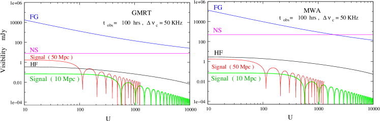
Figure 3: The magnitude of the different contributions to the visibility $V({\vec{U}},\nu)$ at $\nu=153\,{\rm MHz}$ as a function of $U$. The signal, foregrounds (FG), noise (NS) and HI fluctuations (HF) contributions are shown for the GMRT (left) and MWA (right). The expected signal is shown for bubbles with radius $R=10\,\rm{Mpc}$ and $R=50\,\rm{Mpc}$. The noise is estimated for a single baseline assuming an observation time $t_{obs}=100\,{\rm hrs}$ and channel width $\Delta\nu_{c}=50\,{\rm KHz}$.

Contributions from astrophysical foregrounds are expected to be several order of magnitude stronger than the HI signal. Extragalactic point sources and synchrotron radiation from our Galaxy are predicted to be the most dominant foreground components. Assuming that the foregrounds are randomly distributed, with possible clustering, we have $\langle\hat{F}(U,\nu)\rangle=0$ for all the baselines other than the one at zero spacing ($U=0$), which is not considered in this paper. The statistical properties are characterized by the two-visibility correlation $\langle\hat{F}({\vec{U}}_{1},\nu_{1})\hat{F}({\vec{U}}_{2},\nu_{2})\rangle$. We express this (details in Appendix A) in terms of the multi-frequency angular power spectrum (hereafter MAPS) $C_{l}(\nu_{1}\,\nu_{2})$ of the brightness temperature fluctuations at the frequencies $\nu_{1}$ and $\nu_{2}$ as (Santos, Cooray & Knox, 2005; Datta, Choudhury & Bharadwaj, 2006)

$$\langle\hat{F}({\vec{U}}_{1},\nu_{1})\hat{F}({\vec{U}}_{2},\nu_{2})\rangle=\delta_{{\vec{U}}_{1},-{\vec{U}}_{2}}\pi\left(\frac{\theta_{1}^{2}\theta_{2}^{2}}{\theta_{1}^{2}+\theta_{2}^{2}}\right)$$

$$\hskip 56.9055pt\left(\frac{\partial B}{\partial T}\right)_{\nu_{1}}\left(\frac{\partial B}{\partial T}\right)_{\nu_{2}}C_{2\pi U_{1}}(\nu_{1}\,\nu_{2}).$$ (9)

where $(\partial B/\partial T)_{\nu}=2k_{B}\nu^{2}/c^{2}$ is the conversion factor to specific intensity, and we have assumed that the primary beam pattern $A(\theta)=e^{-\theta^{2}/\theta_{0}^{2}}$ is frequency dependent through $\theta_{0}\propto\nu^{-1}$ and use $\theta_{1}$ and $\theta_{2}$ to denote the value of $\theta_{0}$ at $\nu_{1}$ and $\nu_{2}$ respectively. Note that the foreground contribution to different baselines are expected to be uncorrelated.

For each component of the foreground the MAPS is modeled as

$$C_{l}(\nu_{1}\,\nu_{2})=A\left(\frac{\nu_{f}}{\nu_{1}}\right)^{\bar{\alpha}}\left(\frac{\nu_{f}}{\nu_{2}}\right)^{\bar{\alpha}}\left(\frac{1000}{l}\right)^{\beta}I_{l}(\nu_{1}\,\nu_{2}).$$ (10)

where $\nu_{f}=130\,{\rm MHz}$, and for each foreground component $A$, $\beta$ and $\bar{\alpha}$ are the amplitude, the power law index of the angular power spectrum and the mean spectral index respectively. The actual spectral index varies with line of sight across the sky and this causes the foreground contribution to decorrelate with increasing frequency separation $\Delta\nu=|\nu_{1}-\nu_{2}|$ which is quantified through the foreground frequency decorrelation function $I_{l}(\nu_{1}\,\nu_{2})$ (Zaldarriaga, Furlanetto & Hernquist, 2004) which has been modeled as

$$I_{l}(\nu_{1}\,\nu_{2})=\exp\left[-\log_{10}^{2}\left(\frac{\nu_{2}}{\nu_{1}}\right)/2\xi^{2}\right]\,.$$ (11)

We consider the two most dominant foreground components namely extragalactic point sources and the diffuse synchrotron radiation from our own galaxy. Point sources above a flux level $S_{cut}$ can be identified in high-resolution continuum images and removed. We note that absence of large baselines at the MWA restricts the angular resolution, but it may be possible to use the large frequency bandwidth $32\,{\rm MHz}$ to identify continuum point sources in the frequency domain. $S_{cut}$ depends on $\sigma$ the rms. noise in the image. We use $S_{cut}=5\sigma$ where $\sigma$ is the rms noise in the image given by (assuming 2 polarizations)

$$\sigma=\frac{C^{x}}{\sqrt{2N_{b}}}\left(\frac{B}{1\rm{MHz}}\right)^{-1/2}\left(\frac{t_{obs}}{1\rm{sec}}\right)^{-1/2}$$ (12)

where $N_{b}=N(N-1)/2$ is the number of independent baselines, $N$ is the number of antennas in the array, $B$ is the total frequency bandwidth and $t_{obs}$ the total observation time. For $t_{obs}=100\,{\rm hrs}$ and $B=6\,{\rm MHz}$ we have $S_{cut}=0.1{\rm mJy}$ for the GMRT and using $B=32\,{\rm MHz}$ it gives $S_{cut}=0.2\,{\rm mJy}$ for the MWA. The value of $S_{cut}$ will be smaller for longer observations, but reducing $S_{cut}$ any further does not make any difference to our results so we hold $S_{cut}$ fixed at these values for the rest of our analysis. The confusion noise from the unresolved point sources is a combination of two parts, the Poisson contribution due to the discrete nature of these sources and the clustering contribution. The amplitude of these two contributions have different $S_{cut}$ dependence. The parameter values that we have used are listed in Table 1. We have adopted the parameter values from Santos, Cooray & Knox (2005) and incorporated the $S_{cut}$ dependence from DiMatteo. et al. (2002).

Table 1: Parameters values used for characterizing different foreground contributions

Foregrounds	$A({\rm mK^{2}})$	$\bar{\alpha}$	$\beta$	$\xi$
Galactic synchrotron	$700$	$2.80$	$2.4$	$4$
Point source	$61\left(\frac{S_{cut}}{0.1{\rm mJy}}\right)^{0.5}$	$2.07$	$1.1$	$2$
(clustered part)
Point source	$0.16\left(\frac{S_{cut}}{0.1{\rm mJy}}\right)^{1.25}$	$2.07$	$0$	$1$
(Poisson part)

Figure 3 shows the expected foreground contributions for the GMRT and MWA. The galactic synchrotron radiation is the most dominant foreground component at large angular scales ($U<1000$ for GMRT and $U<2000$ for MWA), while the clustering of the unresolved extragalactic point sources dominates at small angular scales. For all values of $U$, the foregrounds are at least four orders of magnitude larger than the signal, and also considerably larger than the noise.

The MWA has been designed with the detection of the statistical HI fluctuation signal in mind, and hence it is planned to have a very large field of view. The foreground contribution to a single baseline is expected to be $~{}10$ times stronger for the MWA than for the GMRT because of a larger field of view. As we shall show later, the increased foreground contribution is not a limitation for detecting HII bubbles. The foregrounds have a continuum spectra, and the contribution at two different frequencies at a separation $\Delta\nu$ are expected to be highly correlated. For $\Delta\nu=1\,{\rm MHz}$, the foreground decorrelation function $I_{l}(\Delta\nu)$ falls by only $2\times 10^{-6}$ for the galactic synchrotron radiation and by $3\times 10^{-5}$ for the point sources. In contrast, the signal from an ionized bubble peaks at a frequency corresponding to the bubble center and falls rapidly with $\Delta\nu$ (Figure 2). This holds the promise of allowing the signal to be separated from the foregrounds.

3 Formalism for detecting the ionized bubble

We consider a radio-interferometric observation of duration $t_{obs}$, carried out over the frequency range $\nu_{1}$ to $\nu_{2}$. The HI signal from an ionized bubble, if it is present in the data, will be buried in foregrounds and noise both of which are expected to be much larger. In this Section we present a filtering technique aimed at detecting the signal from an ionized bubble if it is present in our observations. To detect the signal from an ionized bubble of radius $R_{b}$ with center at redshift $z_{c}$ (or frequency $\nu_{c}$ ) and at an angle $\vec{\theta}_{c}$ from the center of the field of view, we introduce an estimator $\hat{E}[R_{b},z_{c},\vec{\theta}_{c}]$ defined as

$$\hat{E}=\left[\sum_{a,b}S_{f}^{\ast}({\vec{U}}_{a},\nu_{b})\hat{V}({\vec{U}}_{a},\nu_{b})\right]/\left[\sum_{a,b}1\right]$$ (13)

where $S_{f}({\vec{U}},\nu)$ is a filter which has been constructed to detect the particular ionized bubble. Here ${\vec{U}}_{a}$ and $\nu_{b}$ refer to the different baselines and frequency channels in our observations, and in eq. (13) we are to sum over all independent data points (visibilities). Note that the estimator $\hat{E}$ and the filter $S_{f}({\vec{U}},\nu)$ both depend on $[R_{b},z_{c},\vec{\theta}_{c}]$, the parameters of the bubble we wish to detect, but we do not show this explicitly. The values of these parameters will be clear from the context.

We shall be working in the continuum limit where the two sums in eq. (13) can be replaced by integrals and we have

$$\hat{E}=\int d^{2}U\int d\nu\,\rho_{N}({\vec{U}},\nu)\,\,{S_{f}}^{\ast}({\vec{U}},\nu)\hat{V}({\vec{U}},\nu)$$ (14)

$d^{2}Ud\nu\,\rho_{N}({\vec{U}},\nu)$ is the fraction of data points ie. baselines and frequency channels in the interval $d^{2}U\,d\nu$. Note that $\rho_{N}({\vec{U}},\nu)$ is usually frequency dependent, and it is normalized so that $\int d^{2}U\,\int d\nu\,\rho_{N}({\vec{U}},\nu)=1$. We refer to $\rho_{N}({\vec{U}},\nu)$ as the normalized baseline distribution function.

We now calculate $\langle\hat{E}\rangle$ the expectation value of the estimator. Here the angular brackets denote an average with respect different realizations of the HI fluctuations, noise and foregrounds, all of which have been assumed to be random variables with zero mean. This gives $\langle\hat{V}({\vec{U}},\nu)\rangle=S({\vec{U}},\nu)$ and

$$\langle\hat{E}\rangle=\int d^{2}U\,\int d\nu\,\rho_{N}({\vec{U}},\nu)\,\,{S_{f}}^{\ast}({\vec{U}},\nu)S({\vec{U}},\nu)$$ (15)

We next calculate the variance of the estimator which is the sum of the contributions from the noise (NS), the foregrounds(FG) and the HI fluctuations (HF)

$$\langle(\Delta\hat{E})^{2}\rangle \equiv \langle(\hat{E}-\langle\hat{E}\rangle)^{2}\rangle$$

$$= \left<(\Delta\hat{E})^{2}\right>_{{\rm NS}}+\left<(\Delta\hat{E})^{2}\right>_{{\rm FG}}\,+\left<(\Delta\hat{E})^{2}\right>_{{\rm HF}}\,.$$

To calculate the noise contribution we go back to eq. (13) and use the fact that the noise in different baselines and frequency channels are uncorrelated. We have

$$\langle(\Delta\hat{E})^{2}\rangle_{\rm NS}=\langle\hat{N}^{2}\rangle\left[\sum_{a,b}\mid S_{f}({\vec{U}}_{a},\nu_{b})\mid^{2}\right]/\left[\sum_{a,b}1\right]^{2}$$ (17)

which in the continuum limit is

$$\langle(\Delta\hat{E})^{2}\rangle_{\rm NS} = \left[\langle\hat{N}^{2}\rangle/\sum_{a,b}1\right]$$ (18)

$$\times \int d^{2}U\,\int d\nu\,\rho_{N}({\vec{U}},\nu)\,\,\mid S_{f}({\vec{U}},\nu)\mid^{2}$$

The term $\sqrt{\left[\langle\hat{N}^{2}\rangle/\sum_{a,b}1\right]}$ is the same as $\sigma$, the rms. noise in the image (eq. 12). We then have

$$\langle(\Delta\hat{E})^{2}\rangle_{\rm NS}=\sigma^{2}\int d^{2}U\,\int d\nu\,\rho_{N}({\vec{U}},\nu)\,\,\mid S_{f}({\vec{U}},\nu)\mid^{2}\,.$$ (19)

For the foreground contribution we have

$$\left<(\Delta\hat{E})^{2}\right>_{\rm{FG}}\!\!\!\!\! = \!\!\!\!\!\int{\rm d}^{2}U_{1}\int{\rm d}^{2}U_{2}\int{\rm d}\nu_{1}\int{\rm d}\nu_{2}$$ (20)

$$\times \!\!\!\!\!\rho_{N}({\vec{U}}_{1},\nu_{1})\rho_{N}({\vec{U}}_{2},\nu_{2}){S_{f}}^{\ast}({\vec{U}}_{1},\nu_{1}){S_{f}}^{\ast}({\vec{U}}_{2},\nu_{2})$$

$$\times \!\!\!\!\!\langle\hat{F}({\vec{U}}_{1},\nu_{1})\hat{F}({\vec{U}}_{2},\nu_{2})\rangle$$

In the continuum limit we have (details given in Appendix A)

$$\langle\hat{F}({\vec{U}}_{1},\nu_{1})\hat{F}({\vec{U}}_{2},\nu_{2})\rangle = \delta_{D}^{(2)}({\vec{U}}_{1}+{\vec{U}}_{2})\left(\frac{\partial B}{\partial T}\right)_{\nu_{1}}\left(\frac{\partial B}{\partial T}\right)_{\nu_{2}}$$ (21)

$$\times C_{2\pi U_{1}}(\nu_{1},\nu_{2})$$

which gives the variance of the foreground contribution to be

$$\left<(\Delta\hat{E})^{2}\right>_{\rm{FG}}\!\!\!\!\! = \!\!\!\!\!\int{\rm d}^{2}U\int{\rm d}\nu_{1}\int{\rm d}\nu_{2}\left(\frac{\partial B}{\partial T}\right)_{\nu_{1}}\left(\frac{\partial B}{\partial T}\right)_{\nu_{2}}$$ (22)

$$\times \!\!\!\!\!\rho_{N}({\vec{U}},\nu_{1})\rho_{N}({\vec{U}},\nu_{2}){S_{f}}^{\ast}({\vec{U}},\nu_{1}){S_{f}}({\vec{U}},\nu_{2})$$

$$\times \!\!\!\!\!C_{2\pi U}(\nu_{1},\nu_{2})$$

We use eq. (22) to calculate $\left<(\Delta\hat{E})^{2}\right>_{\rm{HF}}$ too, with the difference that we use the power spectrum $C_{2\pi U}(\nu,\nu+\Delta\nu)$ for the HI fluctuation from Datta, Choudhury & Bharadwaj (2006) instead of the foreground contribution.

In an observation it will be possible to detect the presence of an ionized bubble having parameters $[R_{b},z_{c},\vec{\theta}_{c}]$ at, say 3-sigma confidence level, if $\langle\hat{E}\rangle\geq 3\sqrt{\langle(\Delta\hat{E})^{2}\rangle}$. In such a situation, an observed value $E_{o}$ can be interpreted as a detection with $99.7\%$ (i.e., 3-sigma) confidence if $E_{o}>3\sqrt{\langle(\Delta\hat{E})^{2}\rangle}$. The presence of the ionized bubble can be ruled out at the same level of confidence if $\langle\hat{E}\rangle-E_{o}>~{}3~{}\sqrt{\langle(\Delta\hat{E})^{2}\rangle}$.

3.1 Baseline distribution

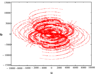
Figure 4: This shows the baseline coverage for $14\,{\rm hrs}$ of GMRT $153\,{\rm MHz}$ observation at $45\degr$ declination.

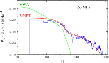
Figure 5: This shows the normalized baseline distribution $\rho_{N}(U,\nu)$ for the GMRT and the MWA at $153\,{\rm MHz}$. The wiggly curve shows the actual values for the GMRT observation shown in Figure 4 and the smooth curve is the analytic fit.

In this subsection we discuss the normalized baseline distribution function $\rho_{N}({\vec{U}},\nu)$ which has been introduced earlier. Figure 4 shows the baseline coverage for $14\,{\rm hrs}$ of observation towards a region at declination $\delta=45\degr$ with the GMRT at $153{\rm MHz}$. In this figure $u$ and $v$ refer to the Cartesian components of the baselines ${\vec{U}}$. Note that the baseline distribution is not exactly circularly symmetric. This asymmetry depends on the source declination which would be different for every observation. We make the simplifying assumption that the baseline distribution is circularly symmetric whereby $\rho_{N}({\vec{U}},\nu)$ is a function of $U$. This considerably simplifies our analysis and gives reasonable estimates of what we would expect over a range of declinations. Figure 5 shows $\rho_{N}({\vec{U}},\nu)$ for the GM RT determined from the baseline coverage shown in Figure 4. We find that this is well described by the sum of a Gaussian and an exponential distribution. The GMRT has a hybrid antenna distribution (Chengalur et al., 2003) with $14$ antennas being randomly distributed in a central square approximately $1\,{\rm km}\times 1\,{\rm km}$ and $16$ antennas being distributed along a Y each of whose arms is $14\,{\rm km}$ long. The Gaussian gives a good fit at small baselines in the central square and the exponential fits the large baselines. Determining the best fit parameters using a least square gives

$$\rho_{N}({\vec{U}},\nu) = \frac{1}{B}\left(\frac{\lambda}{{1\,\rm km}}\right)^{2}\left[0.21\exp\left(-\frac{{U\lambda}}{2a^{2}}\right)\right.$$ (23)

$$+ \left.9.70\times 10^{-3}\exp\left(-\frac{U\lambda-b}{d}\right)\right]$$

where $a=0.382\,{\rm km}$, $b=0.986\,{\rm km}$, $d=3.07\,{\rm km}$ and $B$ is the frequency bandwidth which has a maximum value of $6\,{\rm MHz}$.

Following Bowman et al. (2006) we assume that the MWA antennas are distributed within a radius of $0.750\,{\rm km}$ with the density of antennas decreasing with radius $r$ as $\rho_{ant}(r)\propto r^{-2}$ and with a maximum density of one antenna per $18{\rm m^{2}}$. The normalized baseline distribution is estimated in terms of $\rho_{ant}(r)$ and we have

$$\rho_{N}({\vec{U}},\nu) = \frac{1}{4.4\times 10^{2}}\frac{1}{B}\left(\frac{\lambda}{1\,{\rm km}}\right)^{2}\int_{r=0}^{\infty}{\rm d}^{2}r\rho_{ant}(r)$$ (24)

$$\times \int_{\phi=0}^{2\pi}\rho_{ant}(|{\vec{r}}-\lambda\,{\vec{U}}\,|){\rm d}\phi$$

where the bandwidth $B$ is $32\,{\rm MHz}$, $|{\vec{r}}-\lambda\,{\vec{U}}|=\left(r^{2}+U^{2}\,\lambda^{2}-2r\,\lambda\,U\,cos\phi\right)^{1/2}$. Note that $\rho_{N}({\vec{U}},\nu)$ depends on the observed frequency. Figure 5 shows the normalized baseline distribution function $\rho_{N}({\vec{U}},\nu)$ for both the GMRT and the MWA. We see that maximum baseline for the GMRT is $U_{max}\sim 10,000$ whereas $U_{max}\sim 750$ for the MWA. However, the smaller baselines will be sampled more densely in the MWA as compared to the GMRT.

3.2 Filter

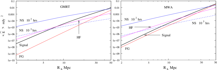
Figure 6: The signal quantified through the expectation value of the estimator $\langle\hat{E}\rangle$ for Filter I. The other components (NS - Noise, FG - Foregrounds, HF - HI Fluctuations) are quantified through their contribution to the 3-sigma fluctuation $3\times\sqrt{\langle(\Delta\hat{E})^{2}\rangle}$.

It is a major challenge to detect the signal which is expected to be buried in noise and foregrounds both of which are much stronger (Figure 3). It would be relatively simple to detect the signal in a situation where there is only noise and no foregrounds. The signal to noise ratio (SNR) is maximum if we use the signal that we wish to detect as the filter ($ie.\,S_{f}({\vec{U}},\nu)=S({\vec{U}},\nu)$) and the SNR has a value

$$\frac{\langle(\hat{E})\rangle}{\sqrt{\langle(\Delta\hat{E})^{2}\rangle_{\rm NS}}}\!\!\!\!\! = \!\!\!\!\!\frac{1}{\sigma}\left[\int\,{\rm d}^{2}U\,\int{\rm d}\nu\,\rho_{N}({\vec{U}},\nu)\mid S({\vec{U}},\nu)\mid^{2}\right]^{0.5}$$ (25)

$$\propto \!\!\!\!\!\sqrt{t_{obs}}\,.$$

The observing time necessary for a $3$-$\sigma$ detection (i.e., SNR $=3$) would be the least for this filter. The difficulty with using this filter is that the foreground contribution to $\sqrt{\langle(\Delta\hat{E})^{2}\rangle}$ is orders of magnitude more than $\langle(\hat{E})\rangle$. The foregrounds, unlike the HI signal, are all expected to have a smooth frequency dependence and one requires filters which incorporate this fact so as to reduce the foreground contribution. We consider two different filters which reduce the foreground contribution, but it occurs at the expense of reducing the SNR, and $t_{obs}$ would be more than that predicted by eq. (25).

The first filter (Filter I) subtracts out any frequency independent component from the frequency range $\nu_{c}-B^{{}^{\prime}}/2$ to $\nu_{c}+B^{{}^{\prime}}/2$ with $B{{}^{\prime}}\leq B$ ie.

$$S_{f}({\vec{U}},\,\nu)\!\!\!\!\! = \!\!\!\!\!\left(\frac{\lambda_{c}}{\lambda}\right)^{2}\left[S({\vec{U}},\,\nu)\right.$$

$$- \!\!\!\!\!\left.\frac{\Theta(1-2\mid\nu-\nu_{c}\mid/B^{{}^{\prime}})}{B^{{}^{\prime}}}\int_{\nu_{c}-B^{{}^{\prime}}/2}^{\nu_{c}+B^{{}^{\prime}}/2}S({\vec{U}},\nu^{\prime})\,{\rm d}\nu^{\prime}\right].$$

This filter has the advantage that it does not require any prior knowledge about the foregrounds except that they have a continuous spectrum. It has the drawback that there will be contributions from the residual foregrounds as all the foregrounds are expected to have a power law spectral dependence and not a constant. A larger value of $B^{{}^{\prime}}$ causes the SNR to increases, and in the limit $B^{{}^{\prime}}\rightarrow{\infty}$ the SNR approaches the value given in eq. (25). Unfortunately the residues in the foregrounds also increase with $B^{{}^{\prime}}$. We use $B^{{}^{\prime}}=4\Delta\nu_{b}$ provided it is less than $B$, and $B^{{}^{\prime}}=B$ otherwise.

The frequency dependence of the total foreground contribution can be expanded in Taylor series. Retaining terms only up to the first order we have

$$C_{l}(\nu_{1},\,\nu_{2})=C_{l}(\nu_{c},\,\nu_{c})\left[1-\left(\Delta\nu_{1}+\Delta\nu_{2}\right)\alpha_{eff}/\nu_{c}\right]$$ (27)

where $\Delta\nu=\nu-\nu_{c}$ and $\alpha_{eff}=\frac{\sum_{i}\alpha^{i}\,A^{i}\left(1000/l\right)^{\beta_{i}}}{\sum_{i}A^{i}\left(1000/l\right)^{\beta_{i}}}$ is the effective spectral index, here $i$ refers to the different foreground components. Note that $\alpha_{eff}$ is $l$ dependent. The second filter that we consider (Filter II) allows for a linear frequency dependence of the foregrounds and we have

$$S_{f}({\vec{U}},\nu)\!\!\!\!\! = \!\!\!\!\!(1+\alpha_{eff}\Delta\nu/\nu_{c})\left(\frac{\lambda_{c}}{\lambda}\right)^{2}\left[S({\vec{U}},\,\nu)\right.$$

$$- \!\!\!\!\!\left.\frac{\Theta(1-2\mid\nu-\nu_{c}\mid/B^{{}^{\prime}})}{B^{{}^{\prime}}}\int_{\nu_{c}-B^{{}^{\prime}}/2}^{\nu_{c}+B^{{}^{\prime}}/2}S({\vec{U}},\nu^{\prime})\,{\rm d}\nu^{\prime}\right].$$

Note that for both the filters we include an extra factor $\left(\lambda_{c}/\lambda\right)^{2}$. This is introduced with the purpose of canceling out the $\lambda^{2}$ dependence of of the normalized baseline distribution function $\rho_{N}({\vec{U}},\nu)$ and this substantially reduces the foreground contribution.

4 Results and Discussions

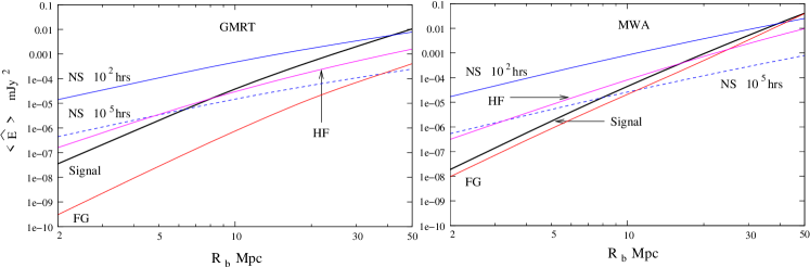
Figure 7: Same as Figure 6 except that Filter II is used instead of Filter I.

We first consider the most optimistic situation where the bubble is at the center of the field of view and the filter center is exactly matched with the bubble center. The size distribution of HII regions are quite uncertain, and would depend on the reionization history and the distribution of ionizing sources. However, there are some indications in the literature on what could be the typical size of HII regions. For example, Wyithe et al. (2005) deduce from proximity zone effects that $R_{b}\approx 35$ Mpc at $z\approx 6$, which should be considered as a lower limit. On the other hand, Furlanetto et al. (2006) (Figure 1(a)) infer that the characteristic bubble size $R_{b}>10\,\rm{Mpc}$ at $z=8$ if the ionized fraction $x_{i}>0.75$ ($R_{b}\sim 50\rm{Mpc}$ if $x_{i}\sim 0.9$). Theoretical models which match a variety of observations (Choudhury & Ferrara, 2007) imply that $x_{i}$ could be as high as $90\,\%$ at $z\sim 8$, which would mean bubble sizes of $\,\sim 40-50$ Mpc. To allow for the large variety of possibilities, we have presented results for a wide range of $R_{b}$ values from $2\,{\rm Mpc}$ to $50\,{\rm Mpc}$. We restrict our analysis to a situation where the IGM outside the bubble is completely neutral ($x_{\rm HI}=1$). The signal would fall proportional to $x_{\rm HI}$ if the IGM outside the bubble were partially ionized ($x_{\rm HI}<1$). The expected signal $\langle\hat{E}\rangle$ and 3-sigma fluctuation $3\times\sqrt{\langle(\Delta\hat{E})^{2}\rangle}$ from each of the different components discussed in Sections 2 and 3 as a function of bubble size $R_{b}$ are shown in Figures 6 and 7. Both the figures show exactly the same quantities, the only difference being that they refer to Filter I and Filter II respectively. A detection is possible only in situations where $\langle\hat{E}\rangle>3\times\sqrt{\langle(\Delta\hat{E})^{2}\rangle}$, the rhs. now refers to the total contribution to the estimator variance from all the components.

The signal is expected to scale as $R_{b}^{3}$ and the noise as $R_{b}^{3/2}$ in a situation where the baseline distribution is uniform ie. $\rho_{N}({\vec{U}},\nu)$ is independent of $U$. This holds at $U<300$ for the GMRT (Figure 5), and the expected scaling is seen for $R_{b}\geq 20\,{\rm Mpc}$. For smaller bubbles the signal extends to larger baselines where $\rho_{N}(U,\nu)$ falls sharply, and the signal and the noise both have a steeper $R_{b}$ dependence. The MWA baseline distribution is flat for only a small $U$ range (Figure 5) beyond which it drops. In this case the signal and noise are found to scale as $R_{b}^{4}$ and $R_{b}^{2}$ respectively. Note that the maximum baseline at MWA is $U=750$, and hence a considerable amount of the signal is lost for $R_{b}<10\,{\rm Mpc}$.

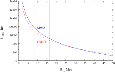
Figure 8: The observing time $t_{obs}$ that would be required for a $3\,\sigma$ detection of a bubble of radius $R_{b}$ provided it is at the center of the field of view. The vertical lines shows the lower limit (due to HI fluctuations) where a detection will be possible ($R_{b}=8\,{\rm Mpc}$ for GMRT and $R_{b}=16\,{\rm Mpc}$ for MWA).

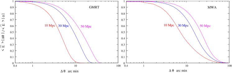
Figure 9: The Overlap between the signal and the filter when there is a mismatch $\Delta\theta$ between the centers of the bubble and the filter for GMRT (left) and MWA (right). The results are shown for different bubble sizes.

At both the GMRT and the MWA, for $100\,{\rm hrs}$ of observation, the noise is larger than the signal for bubble size $R_{b}\leq 40\,{\rm Mpc}$. At the other extreme, for an integration time of $10^{5}\,{\rm hrs}$ the noise is below the signal for $R_{b}>6\,{\rm Mpc}$ for the GMRT and $R_{b}>8\,{\rm Mpc}$ for the MWA. The foreground contribution turns out to be smaller than the signal for the entire range of bubble sizes that we have considered, thus justifying our choice of filters. Note that Filter II is more efficient in foreground subtraction, but it requires prior knowledge about the frequency dependence. For both the filters the foreground removal is more effective at the GMRT than the MWA because of the frequency dependence of $\rho_{N}({\vec{U}},\nu)$. The assumption that this is proportional to $\lambda^{2}$ is valid only when $\rho({\vec{U}},\nu)$ is independent of $U$, which, as we have discussed, is true for a large $U$ range at the GMRT. The $\lambda$ dependence is much more complicated at the MWA, but we have not considered such details here as the foreground contribution is anyway smaller than the signal. It should also be noted that the foreground contribution increases at small baselines (eq. 10), and is very sensitive to the smallest value of $U$ which we set at $U=20$ for our calculations. Here it must be noted that our results are valid only under the assumption that the foregrounds have a smooth frequency dependence. A slight deviation from this and the signal will be swamped by the foregrounds. Also note that this filtering method is effective only for the detection of the bubbles and not for the statistical HI fluctuations signal.

The contribution from the HI fluctuations impose a lower limit on the size of the bubble which can be detected. However long be the observing time, it will not be possible to detect bubbles of size $R_{b}<8\,{\rm Mpc}$ using the GMRT and size $R_{b}<16\,{\rm Mpc}$ using the MWA. The HI fluctuation contribution increases at small baselines. The problem is particularly severe at MWA because of the dense sampling of the small baselines and the very large field of view. We note that the MWA is being designed with the detection of the statistical HI fluctuation signal in mind, and hence it is not surprising that this contribution is quite large. For both telescopes it may be possible to reduce this component by cutting off the filter at small baselines. We have not explored this possibility in this work because the enormous observing times required to detect such small bubbles makes it unfeasible with the GMRT or MWA.

Figure 8 shows the observation time that would be required to detect bubbles of different sizes using Filter I for GMRT and the MWA. Note that the observing time shown here refers to a $3\,\sigma$ detection which is possibly adequate for targeted searches centered on observed quasar position. A more stringent detection criteria at the $5\,\sigma$ level would be apropriate for a blind search. The observing time would go up by a factor of $3$ for a $5\,\sigma$ detection. The observing time is similar for Filter II and hence we do not show this separately. In calculating the observing time we have only taken into account the noise contribution as the other contributions do not change with time. The value of $R_{b}$ below which a detection is not possible due to the HI fluctuations is shown by vertical lines for both telescopes. We see that with $100\,{\rm hrs}$ of observation both the telescopes will be able to detect bubbles with $R_{b}>40\,{\rm Mpc}$ while bubbles with $R_{b}>22{\rm Mpc}$ can be detected with $1000\,{\rm hrs}$ of observation.

The possibility of detecting a bubble is less when the bubble centre does not coincide with the centre of the field of view. In fact, the SNR falls as $e^{-\theta_{c}^{2}/\theta_{0}^{2}}$ if the bubble center is shifted away by $\theta_{c}$ from the center of the field of view and the filter is also shifted so that its center coincides with that of the bubble. There will be a corresponding increase $t_{obs}\propto e^{2\theta_{c}^{2}/\theta_{0}^{2}}$ in the observing time required to detect the bubble. It will be possible to detect bubbles only if they are located near the center of the field of view ($\theta_{c}\ll\theta_{0}$), and the required observing time increases rapidly with $\theta_{c}$ for off-centered bubbles.

When searching for bubbles in a particular observation it will be necessary to consider filters corresponding to all possible value of $R_{b}$, $\nu_{c}$ and $\vec{\theta}_{c}$. A possible strategy would be to search at a discrete set of values in the range of $R_{b}$, $\nu_{c}$ and $\vec{\theta}_{c}$ values where a detection is feasible. The crucial issue here would be the choice of the sampling density so that we do not miss out an ionized bubble whose parameters do not exactly coincide with any of the values in the discrete set and lie somewhere in between. To illustrate this we discuss the considerations for choosing and optimal value of $\Delta\theta_{c}$ the sampling interval for $\vec{\theta}_{c}$. We use $\langle\hat{E}\rangle[\Delta\theta]$ to denote the expectation value of the estimator when there is a mismatch $\Delta\theta$ between the centers of the bubble and the filter. The ratio ${\rm Overlap}=\langle\hat{E}\rangle[\Delta\theta]/\langle\hat{E}\rangle[0]$, shown in Figure 9 for GMRT (left panel) and MWA (right panel), quantifies the overlap between the signal and the filter as $\Delta\theta$ is varied. We see that the choice of $\Delta\theta$ would depend on the size of the bubble we are trying to detect and it would be smaller for the GMRT as compared to the MWA. Permitting the Overlap to drop to $0.9$ at the middle of the sampling interval, we find that it is $8^{{}^{\prime}}$ at the GMRT and $20^{{}^{\prime}}$ at the MWA for $R_{b}=50\,{\rm Mpc}$.

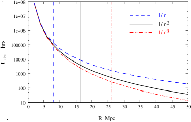
Figure 10: Same as the Figure 8 considering three different antenna distributions $\rho_{ant}(r)\propto 1/r$,  $1/r^{2}$,  $1/r^{3}$   for the MWA.

The MWA is yet to be constructed, and it may be possible that an antennae distribution different from $\rho_{ant}(r)\propto 1/r^{2},\,$ may improve the prospects of detecting HII bubbles. We have tried out $\rho_{ant}(r)\propto 1/r\,{\rm and}\,1/r^{3}$ for which the results are shown in Figure 10. We find that the required integration time falls considerably for the $1/r^{3}$ distribution whereas the opposite occurs for $1/r$. For example, for $R_{b}=50\,{\rm Mpc}$ the integration time increases by $5$ times for $1/r$ and decreases by $3$ times for $1/r^{3}$ as compared to $1/r^{2}$. Based on this we expect the integration time to come down if the antenna distribution is made steeper, but this occurs at the expense of increasing the HI fluctuations and the foregrounds. We note that for the $1/r^{3}$ distribution the foreground contribution is more than the signal, but it may be possible to overcome this by modifying the filter. The increase in the HI fluctuations is inevitable, and it restricts the smallest bubble that can be detected to $R=26\,{\rm MPc}$ for $1/r^{3}$. In summary, the $1/r^{2}$ distribution appears to be a good compromise between reducing the integration time and increasing the HI fluctuations and foregrounds.

Finally we examine some of the assumptions made in this work. First, the Fourier relation between the specific intensity and the visibilities (eq. 1) will be valid only near the center of the field of view and full three dimensional wide-field imaging is needed away from the center. As the feasibility of detecting a bubble away from the center falls rapidly, we do not expect the wide-field effects to be very important. Further, these effects are most significant at large baselines whereas most of the signal from ionized bubbles is in the small baselines.

Inhomogeneities in the IGM will affect the propagation of ionization fronts, and the ionized bubbles are not expected to be exactly spherical (Wyithe et al., 2005). This will cause a mismatch between the signal and the filter which in turn will degrade the SNR. In addition to this, in future we plan to address a variety of other issues like considering different observing frequencies and making predictions for the other upcoming telescopes.

Terrestrial signals from television, FM radio, satellites, mobile communication etc., collectively referred to as RFI, fall in the same frequency band as the redshifted $21\rm cm$ signal from the reionization epoch. These are expected to be much stronger than the expected $21{\rm cm}$ signal, and it is necessary to quantify and characterize the RFI. Recently Bowman et al. (2007) have characterized the RFI for the MWA site on the frequency range $80$ to $300\rm MHz$. They find an excellent RFI environment except for a few channels which are dominated by satellite communication signal. The impact of RFI on detecting ionized bubbles is an important issue which we plan to address in future.

The effect of polarization leakage is another issue we postpone for future work. This could cause polarization structures on the sky to appear as frequency dependent ripples in the foregrounds intensity . This could be particularly severe for the MWA.

Appendix A Relation between visibility-visibility correlation and MAPS

In this appendix we give the calculations for expressing the two visibility correlation in terms of the Multi-frequency angular power spectrum (MAPS). We can write the visibility $V({\vec{U}},\nu)$ as a two-dimensional Fourier transform of the brightness temperature $T(\vec{\theta},\nu)$ [see equation (1)]

$$V({\vec{U}},\nu)=\left(\frac{\partial B}{\partial T}\right)_{\nu}\int d^{2}\theta A(\vec{\theta},\nu)T(\vec{\theta},\nu)e^{2\pi\imath\vec{\theta}\cdot{\vec{U}}}$$ (29)

where $(\partial B/\partial T)_{\nu}$ is the conversion factor from temperature to specific intensity and $A(\vec{\theta},\nu)$ is the beam pattern of the individual antenna. The visibility-visibility correlation is then given by

$$\langle V({\vec{U}}_{1},\nu_{1})V({\vec{U}}_{2},\nu_{2})\rangle\!\!\!\!\! = \!\!\!\!\!\left(\frac{\partial B}{\partial T}\right)_{\nu_{1}}\left(\frac{\partial B}{\partial T}\right)_{\nu_{2}}$$

$$\times \!\!\!\!\!\int d^{2}\theta\int d^{2}\theta^{\prime}A(\vec{\theta},\nu_{1})A(\vec{\theta}^{\prime},\nu_{2})$$

$$\times \!\!\!\!\!\langle T(\vec{\theta},\nu_{1})T(\vec{\theta}^{\prime},\nu_{2})\rangle e^{2\pi\imath(\vec{\theta}\cdot{\vec{U}}_{1}+\vec{\theta}^{\prime}\cdot{\vec{U}}_{2})}$$

The correlation function for the temperature fluctuations on the sky would simply be the two-dimensional Fourier transform of the MAPS $C_{2\pi U}(\nu_{1},\nu_{2})$

$$\langle T(\vec{\theta},\nu_{1})T(\vec{\theta}^{\prime},\nu_{2})\rangle=\int d^{2}U~{}C_{2\pi U}(\nu_{1},\nu_{2})e^{-2\pi\imath(\vec{\theta}-\vec{\theta}^{\prime})\cdot{\vec{U}}}$$ (31)

Using the above equation in equation in (LABEL:eq:vis-vis), we obtain

$$\langle V({\vec{U}}_{1},\nu_{1})V({\vec{U}}_{2},\nu_{2})\rangle\!\!\!\!\! = \!\!\!\!\!\left(\frac{\partial B}{\partial T}\right)_{\nu_{1}}\left(\frac{\partial B}{\partial T}\right)_{\nu_{2}}$$ (32)

$$\times \!\!\!\!\!\int d^{2}U~{}C_{2\pi U}(\nu_{1},\nu_{2})$$

$$\times \!\!\!\!\!\tilde{A}({\vec{U}}_{1}-{\vec{U}},\nu_{1})\tilde{A}({\vec{U}}_{2}+{\vec{U}},\nu_{2})$$

where $\tilde{A}({\vec{U}},\nu)$ is the Fourier transform of the beam pattern $A(\vec{\theta},\nu)$. If the beam pattern is assumed to be Gaussian $A(\vec{\theta},\nu)=e^{-\theta^{2}/\theta_{0}^{2}}$, the Fourier transform too is given by a Gaussian function

$$\tilde{A}({\vec{U}},\nu)=\pi\theta_{0}^{2}e^{-\pi^{2}U^{2}\theta_{0}^{2}}$$ (33)

Hence, the visibility correlation becomes

$$\langle V({\vec{U}}_{1},\nu_{1})V({\vec{U}}_{2},\nu_{2})\rangle\!\!\!\!\! = \!\!\!\!\!\left(\frac{\partial B}{\partial T}\right)_{\nu_{1}}\left(\frac{\partial B}{\partial T}\right)_{\nu_{2}}\pi^{2}\theta_{1}^{2}\theta_{2}^{2}$$ (34)

$$\times \!\!\!\!\!\int d^{2}U~{}C_{2\pi U}(\nu_{1},\nu_{2})$$

$$\times \!\!\!\!\!e^{-\pi^{2}[({\vec{U}}_{1}-{\vec{U}})^{2}\theta_{1}^{2}+({\vec{U}}_{2}+{\vec{U}})^{2}\theta_{2}^{2}]}$$

where $\theta_{1}$ and $\theta_{2}$ are the values of $\theta_{0}$ at $\nu_{1}$ and $\nu_{2}$ respectively. Now, since the two Gaussian functions in the above equation is peaked around different values of ${\vec{U}}$, the integrand will have a non-zero contribution only when $|{\vec{U}}_{1}+{\vec{U}}_{2}|<(\pi~{}{\rm max}[\theta_{1},\theta_{2}])^{-1}$. In case the typical baselines are much larger than the quantity $(\pi~{}{\rm max}[\theta_{1},\theta_{2}])^{-1}$, the integral above can be well approximated as being non-zero only when ${\vec{U}}_{1}=-{\vec{U}}_{2}$. Then

$$\langle V({\vec{U}}_{1},\nu_{1})V({\vec{U}}_{2},\nu_{2})\rangle\!\!\!\!\! \approx \!\!\!\!\!\delta_{{\vec{U}}_{1},-{\vec{U}}_{2}}\left(\frac{\partial B}{\partial T}\right)_{\nu_{1}}\left(\frac{\partial B}{\partial T}\right)_{\nu_{2}}$$ (35)

$$\times \!\!\!\!\!\pi^{2}\theta_{1}^{2}\theta_{2}^{2}C_{2\pi U_{1}}(\nu_{1},\nu_{2})$$

$$\times \!\!\!\!\!\int d^{2}Ue^{-\pi^{2}[({\vec{U}}_{1}-{\vec{U}})^{2}(\theta_{1}^{2}+\theta_{2}^{2})]}$$

$$= \!\!\!\!\!\delta_{{\vec{U}}_{1},-{\vec{U}}_{2}}\pi\left(\frac{\theta_{1}^{2}\theta_{2}^{2}}{\theta_{1}^{2}+\theta_{2}^{2}}\right)\left(\frac{\partial B}{\partial T}\right)_{\nu_{1}}\left(\frac{\partial B}{\partial T}\right)_{\nu_{2}}$$

$$\times \!\!\!\!\!C_{2\pi U_{1}}(\nu_{1},\nu_{2})$$

which is what has been used in equation (9).

In the continuum limit, the Gaussian $\tilde{A}({\vec{U}},\nu)$ can be approximated by a delta function, i.e., $\tilde{A}({\vec{U}},\nu)\approx\delta^{(2)}_{D}({\vec{U}})$ (which corresponds to the limit $\theta_{0}\to\infty$); the visibility-visibility correlation is then given as

$$\langle V({\vec{U}}_{1},\nu_{1})V({\vec{U}}_{2},\nu_{2})\rangle=\delta^{(2)}_{D}({\vec{U}}_{1}+{\vec{U}}_{2})\left(\frac{\partial B}{\partial T}\right)_{\nu_{1}}\left(\frac{\partial B}{\partial T}\right)_{\nu_{2}}$$

$$\times C_{2\pi U_{1}}(\nu_{1},\nu_{2})$$ (36)

which corresponds to equation (21) in the main text.

References

- Barkana & Loeb (2001) Barkana R. & Loeb A., 2001, Phys.Rep., 349, 125
- Becker et al. (2001) Becker, R.H., et al., 2001, AJ, 122, 2850
- Bharadwaj & Ali (2004) Bharadwaj, S., & Ali, S. S. 2004, MNRAS, 352, 142
- Bharadwaj & Ali (2005) Bharadwaj, S., & Ali, S. S. 2005, MNRAS, 356, 1519
- Bharadwaj & Pandey (2005) Bharadwaj, S., & Pandey, S. K. 2005, MNRAS, 358, 968
- Bowman et al. (2006) Bowman, J. D., Morales, M. F., & Hewitt, J. N. 2006, ApJ, 638, 20
- Bowman et al. (2007) Bowman, J. D. et. al.,2006, Preprint: astro-ph/0611751
- Chengalur et al. (2003) Chengalur, J.N., Gupta, Y., & Dwarkanath, K.S., 2003, Low frequency Radio Astronomy , pp.191
- Choudhury & Ferrara (2006a) Choudhury T. R., Ferrara A., Preprint: astro-ph/0603149, 2006a
- Choudhury & Ferrara (2007) Choudhury T. R., Ferrara A., Preprint: astro-ph/0703771, 2007
- Cooray & Furlanetto (2004) Cooray, A., & Furlanetto, S. R. 2004, ApJL, 606, L5
- Datta, Choudhury & Bharadwaj (2006) Datta, K. K., Choudhury, T., R., & Bharadwaj, S. 2006,astro-ph/0605546
- DiMatteo. et al. (2002) DiMatteo,T., Perna R., Abel,T., Rees,M.J. 2002, ApJ, 564, 576
- Fan, Carilli & Keating (2006) Fan, X., C. L. Carilli, and B. Keating, Preprint: astro-ph/0602375, 2006.
- Fan et al. (2002) Fan, X., et al. 2002, AJ, 123, 1247
- Furlanetto, Zaldarriaga & Hernquist (2004) Furlanetto, S. R., Zaldarriaga, M., & Hernquist, L. 2004a, ApJ, 613, 1
- Furlanetto et al. (2006) Furlanetto, S. R., McQuinn, M., & Hernquist, L. 2006, MNRAS, 365, 115
- Furlanetto et al. (2006) Furlanetto, S. R., Oh, S. P., & Briggs, F. H. 2006, Physics Report, 433, 181
- Morales & Hewitt (2004) Morales, M. F., & Hewitt, J. 2004, ApJ, 615, 7
- Oh (1999) Oh, S. P. 1999, ApJ, 527, 16
- Page et al. (2006) Page, L. et al., 2006, Preprint: astro-ph/0603450
- Santos, Cooray & Knox (2005) Santos, M. G., Cooray, A., & Knox, L. 2005, ApJ, 625, 575
- Shaver et al. (1999) Shaver, P. A., Windhorst, R, A., Madau, P.& de Bruyn, A. G., 1999, Astron. & Astrophys.,345,380
- Spergel et al. (2006) Spergel, D. N.,et al. 2006,astro-ph/0603449
- Swarup et al. (1991) Swarup G., Ananthakrishnan S., Kapahi V.K., Rao A.P., Subramanya C.R., Kulkarni V.K.,1991 Curr.Sci.,60,95
- Thompson, Moran & Swenson (1986) Thompson, A.R., Moran, J.M., & Swenson, G.W. 1986, Interferometry and Synthesis in Radio Astronomy, John Wiley & Sons, pp. 160
- Wyithe & Loeb (2004) Wyithe, J. S. B., & Loeb, A. 2004, ApJ, 610, 117
- Wyithe et al. (2005) Wyithe, J. S. B., Loeb, A., & Barnes, D. G. 2005, ApJ, 634, 715
- Zaldarriaga, Furlanetto & Hernquist (2004) Zaldarriaga, M., Furlanetto, S. R., & Hernquist, L. 2004, ApJ, 608, 622