Improved tests on the relationship between the kinetic energy of galaxies and the mass of their central black holes

Abstract

We support, with new fitting instruments and the analysis of more recent experimental data, the proposal of a relationship between the mass of a Supermassive Black Hole (SMBH) and the kinetic energy of random motions in the host elliptical galaxy. The first results obtained in a previous paper with 13 elliptical galaxies are now confirmed by the new data and an enlarged sample. We find $M_{BH}\propto(M_{G}\sigma^{2}/c^{2})^{\beta}$ with $0.8\leq\beta\leq 1$ depending on the different fitting methods and samples used. The meaningful case $\beta=1$ is carefully analyzed. Furthermore, we test the robustness of our relationship including in the sample also lenticular and spiral galaxies and we show that the result does not change. Finally we find a stronger correlation between the mass of the galaxy and the corresponding velocity dispersion that allows to connect our relationship to the $M_{BH}\propto\sigma^{\alpha}$ law. With respect to this law, our relationship has the advantage to have a smaller scatter.

keywords: black hole physics – galaxies: kinematics and dynamics

1 Introduction

In the last ten years the existence of Supermassive Black Holes in the central part of an increasing number of galaxies has become a stronger and stronger evidence. In order to understand the formation process and the evolution of those black holes, it is important to relate them to the properties of the host galaxy. It was shown that the existence of a central SMBH affects the dynamics not only in the core of the host galaxy but even in a region far from the hole. Several relationships have been recently proposed between the mass of a central SMBH and the velocity dispersion [1, 2, 3], the bulge luminosity or mass [4, 5, 6, 7, 8, 9, 10] or the dark matter halo [11], of the corresponding galaxy. Among them, the relationship with the smallest scatter is

$$M_{BH}\propto\sigma^{\alpha}$$

where $3.75<\alpha<5.3$. The different values of $\alpha$, found by several authors using different samples and different fitting methods, are well discussed in the paper of Tremaine et al. [3] that obtain

$$LogM_{BH}=(4.02\pm 0.32)Log(\sigma/200)+(8.13\pm 0.06)$$

where (and also afterwards in the rest of our paper) $M_{BH}$ is expressed in solar masses, $\sigma$ in $km/s$ and logarithms are base 10.

From the theoretical point of view there are still different interpretations of these results [12, 13, 14, 15] and in order to give a contribution to this open debate, in a previous paper [16], we proposed to study a relationship between the kinetic energy of random motions of elliptical galaxies and the rest energy of their central Supermassive Black Hole. We used a sample formed by the intersection between the set of galaxies studied by Tremaine et al. [3] and the kinematical data extracted by [17, 18, 19] that refer to the effective semimajor axis of each galaxy $A_{e}$ (related to the effective radius $R_{e}$ by the formula

$$\frac{R_{e}}{A_{e}}=1-\frac{\epsilon}{2}$$

where $\epsilon$ is the ellipticity). The model used to compute the kinematical parameters is very simple. Busarello, Longo and Feoli [17] assumed that an elliptical galaxy

1. has a spheroidal symmetry,

2. follows the de Vaucouleurs $r^{1/4}$ law,

3. its rotation axis is perpendicular to the line of sight,

4. its stars have a rotation velocity with cylindrical symmetry and

5. its velocity dispersion tensor is isotropic and has spherical symmetry.

The details of the procedure used to compute velocity dispersions, rotation velocities and the masses of the 13 elliptical galaxies included in the so called sample A (see Table 1) were fully explained in [17, 18] and summarized in our previous paper [16] (hereafter AFDM).

Our first results were very encouraging because we found, taking into account errors in both variables and using an iterative procedure due to Orear [20]:

$$Log(M_{BH})=(0.88\pm 0.06)Log\frac{M_{G}\sigma^{2}}{c^{2}}+(4.30\pm 0.46)$$

with (see Appendix for definitions) $\chi^{2}_{r}=2.2$ and with a linear correlation coefficient $r=0.833$. If the Akritas and Bershadi method [21] is used, the slope of the relationship is even closer to unity:

$$Log(M_{BH})=(0.98\pm 0.09)Log\frac{M_{G}\sigma^{2}}{c^{2}}+(3.8\pm 0.4)$$

with $\chi^{2}_{r}=1.9$.

Even better results can be obtained using a reduced sample (hereafter SAMPLE B) of galaxies if we eliminate the two ellipticals with the largest residuals N821 and N4697. The relationships obtained applying the fitting procedure to the remaining 11 galaxies are listed in AFDM. The satisfying results are the increase of the correlation coefficient, the decrease of $\chi^{2}$, and a slope closer to unity.

In order to understand better the origin of this relationship, we have performed in this paper four new tests:

1. We used the well known iterative procedure of FITEXY routine (we had never used before) to analyze again the same samples A and B of the previous paper AFDM in the case of errors in both variables;

2. The simplest hypothesis of a linear relationship was tested using the exact ”least-squares” fitting method;

3. The kinematical data used in the previous paper were extracted by old sources so we have performed a check of the relationship using the data recently published by Häring and Rix [8].

4. In AFDM we have considered only elliptical galaxies. In this paper we tested the robustness of the relationship, including in the statistical analysis also the lenticular and spiral galaxies of the sample published by Häring and Rix [8].

There is another remarkable novelty contained in this paper. Actually in AFDM we found a very poor correlation between the mass of the galaxy and its velocity dispersion. On the contrary with the sample of Häring and Rix [8] this relationship is stronger and we will show that if

$$M_{BH}\propto\sigma^{\alpha}$$

and

$$M_{BH}c^{2}\propto(M_{G}\sigma^{2})^{\beta}$$

then (as we expected) a relation

$$M_{G}\propto\sigma^{\gamma}$$

is such that

$$\gamma=\frac{\alpha}{\beta}-2$$

Furthermore, using the new data, we will show that the equation (7) has a $\chi^{2}$ smaller than the relation (6).

2 The samples

The old data.

(1)	(2)	(3)	(4)	(5)	(6)
Galaxy	$M_{BH}$	$\sigma$	V	$M_{G}$	$\frac{\Delta M_{G}}{M_{G}}$
	($M_{\odot}$)	(km/s)	(km/s)	($M_{\odot}$)
N221	$2.5\times 10^{6}$	60	37	$4.0\times 10^{8}$	0.07
N821	$3.7\times 10^{7}$	180	117	$1.4\times 10^{11}$	0.04
N2778	$1.4\times 10^{7}$	140	96	$4.0\times 10^{10}$	0.16
N3379	$1.0\times 10^{8}$	193	53	$3.0\times 10^{10}$	0.12
N4291	$3.1\times 10^{8}$	250	76	$9.0\times 10^{10}$	0.05
N4473	$1.1\times 10^{8}$	191	62	$7.0\times 10^{10}$	0.16
N4486	$3.0\times 10^{9}$	269	20	$3.5\times 10^{11}$	0.10
N4564	$5.6\times 10^{7}$	125	143	$5.0\times 10^{10}$	0.16
N4649	$2.0\times 10^{9}$	224	56	$2.2\times 10^{11}$	0.51
N4697	$1.7\times 10^{8}$	177	151	$2.9\times 10^{11}$	0.19
N4742	$1.4\times 10^{7}$	81	91	$1.0\times 10^{10}$	0.17
N5845	$2.4\times 10^{8}$	236	73	$2.0\times 10^{10}$	0.16
N6251	$5.3\times 10^{8}$	288	54	$2.3\times 10^{11}$	0.12
IC1459	$2.5\times 10^{9}$	282	383	$3.5\times 10^{11}$	0.03

Table 1: We list in column (1) the name of the galaxy, in column (2) the black hole masses taken from Tremaine et al. [3]. The velocity dispersions (column 3) and the rotation velocities (column 4) are taken from Busarello, Feoli and Longo [17], the masses in column (5) from Curir et al.[19] and the corresponding relative errors in column (6) from Busarello and Longo [18]. The sources of the experimental data for each galaxy are listed in the above mentioned papers.

We decide to adopt in the sample A and B the kinematical parameters computed by Busarello et al. and published for $\sigma$ and $V$ of 54 elliptical galaxies in [17] and for the mass and the specific angular momentum in [18, 19]. These have the advantage to be treated with the same method and the same fitting procedure; furthermore they are all referred to the effective semimajor axis, and are corrected for one projection effect: the integration of the light along the line of sight. All the masses are computed using the same method that is the Jeans equation describing the equilibrium of a spheroidally symmetric system having an isotropic velocity dispersion tensor. The intersection between the set of elliptical galaxies studied in [17, 18, 19] and the set of SMBH masses in Table 1 in the paper of Tremaine et al. [3] leads to 13 galaxies (the elliptical N221 was eliminated because it has a very low velocity dispersion and a mass two orders of magnitude less than all the others) that are listed in Table 1 where $V$ is the luminosity weighted mean rotation velocity inside $A_{e}$ (related to the rotational kinetic energy by $T_{V}=MV^{2}/2$) and

$$\sigma^{2}\equiv<\sigma^{2}_{yy}>=\frac{\int\sigma^{2}_{yy}(r)\rho d^{3}x}{\int\rho d^{3}x}=\frac{2T_{\sigma}}{3M}$$

is the luminosity weighted mean of the line of sight component, of the velocity dispersion tensor, assuming that the mass-to-light ratio is constant inside $A_{e}$ and that the tensor is isotropic ($T_{\sigma}$ is the corresponding kinetic energy).

The sample A is formed by all these 13 galaxies while, as in AFDM, we will denote with sample B the set obtained from A eliminating the galaxies: N821 and N4697.

In order to check our new relationship with a set of more recent data, we extract from the Table 1 of the paper of Häring and Rix [8] the values listed in the first part of our Table 2, including 18 elliptical galaxies (all the ellipticals except N221) that form our sample C. If we add also the remaining eleven non elliptical galaxies of Häring and Rix [8], we obtain our largest sample D. Finally we will study with the new data of Table 2 the same set of galaxies of the sample A and B and we will denote the corresponding samples with $A^{\prime}$ and $B^{\prime}$. Of course the methods used to compute velocity dispersions and Bulge masses by Häring and Rix [8] are often different from Busarello et al. and the data do not refer to the semimajor axis of each galaxy but can extend also to a bulge region of radius $3R_{e}$. This justifies that sometime there are significant differences in the values of the parameters found in the two tables for the same galaxies. For the masses of Black Holes we have preferred to use all the set in [3] even if, for a few galaxies, now some updated values exist, measured by other authors.

The new data.

(1)	(2)	(3)	(4)	(5)	(6)
Galaxy	Type	$M_{BH}$	$\Delta M_{BH}$	$\sigma$	$M_{G}$
		($M_{\odot}$)	($M_{\odot}$)	(km/s)	($M_{\odot}$)
N821	E4	$3.7\times 10^{7}$	$2.4\times 10^{7}$	209	$1.3\times 10^{11}$
N2778	E2	$1.4\times 10^{7}$	$0.9\times 10^{7}$	175	$7.6\times 10^{10}$
N3377	E5	$1.0\times 10^{8}$	$0.9\times 10^{8}$	145	$1.6\times 10^{10}$
N3379	E1	$1.0\times 10^{8}$	$0.6\times 10^{8}$	206	$6.8\times 10^{10}$
N3608	E2	$1.9\times 10^{8}$	$1.0\times 10^{8}$	182	$9.7\times 10^{10}$
N4261	E2	$5.2\times 10^{8}$	$1.1\times 10^{8}$	315	$3.6\times 10^{11}$
N4291	E2	$3.1\times 10^{8}$	$2.3\times 10^{8}$	242	$1.3\times 10^{11}$
N4374	E1	$4.3\times 10^{8}$	$3.2\times 10^{8}$	296	$3.6\times 10^{11}$
N4473	E5	$1.1\times 10^{8}$	$7.9\times 10^{7}$	190	$9.2\times 10^{10}$
N4486	E0	$3.0\times 10^{9}$	$1.0\times 10^{9}$	375	$6.0\times 10^{11}$
N4564	E3	$5.6\times 10^{7}$	$0.8\times 10^{7}$	162	$4.4\times 10^{10}$
N4649	E1	$2.0\times 10^{9}$	$0.6\times 10^{9}$	375	$4.9\times 10^{11}$
N4697	E4	$1.7\times 10^{8}$	$0.2\times 10^{8}$	177	$1.1\times 10^{11}$
N4742	E4	$1.4\times 10^{7}$	$0.5\times 10^{7}$	90	$6.2\times 10^{9}$
N5845	E3	$2.4\times 10^{8}$	$1.4\times 10^{8}$	234	$3.7\times 10^{10}$
N6251	E2	$5.3\times 10^{8}$	$1.8\times 10^{8}$	290	$5.6\times 10^{11}$
N7052	E4	$3.3\times 10^{8}$	$2.3\times 10^{8}$	266	$2.9\times 10^{11}$
IC1459	E3	$2.5\times 10^{9}$	$0.5\times 10^{9}$	323	$2.9\times 10^{11}$
N224	Sb	$4.5\times 10^{7}$	$4.0\times 10^{7}$	160	$3.7\times 10^{10}$
N1023	SB0	$4.4\times 10^{7}$	$0.5\times 10^{7}$	205	$6.9\times 10^{10}$
N1068	Sb	$1.5\times 10^{7}$	$1.5\times 10^{7}$	151	$2.3\times 10^{10}$
N3115	S0	$1.0\times 10^{9}$	$1.0\times 10^{9}$	230	$1.2\times 10^{11}$
N3245	S0	$2.1\times 10^{8}$	$0.5\times 10^{8}$	205	$6.8\times 10^{10}$
N3384	S0	$1.6\times 10^{7}$	$0.2\times 10^{7}$	143	$2.0\times 10^{10}$
N4342	S0	$3.0\times 10^{8}$	$1.7\times 10^{8}$	225	$1.2\times 10^{10}$
N4594	Sa	$7.8\times 10^{7}$	$4.2\times 10^{7}$	240	$2.7\times 10^{11}$
N7332	S0	$1.3\times 10^{7}$	$0.6\times 10^{7}$	122	$1.5\times 10^{10}$
N7457	S0	$3.5\times 10^{6}$	$1.4\times 10^{6}$	67	$7.0\times 10^{09}$
Milky Way	SBbc	$1.8\times 10^{6}$	$0.4\times 10^{6}$	75	$1.1\times 10^{10}$

Table 2: We list in column (1) the name of the galaxy, in column (2) the morphological type from de Vaucouleurs et al.[22], in column (3) the black hole masses and in column (4) the corresponding errors both taken from Tremaine et al. [3] (except for N4374, N4594 and N7332 taken from [8]), in column (5) the stellar velocity dispersions and in column (6) the galaxy masses both taken from Häring and Rix [8]. The sources of the experimental data for each galaxy are listed in the above cited papers.

3 The new results

We start using Fitexy Routine to take into account errors on both variables. We apply it to our six samples of galaxies and the results are reported in Table 3.

(1)	(2)	(3)	(4)	(5)	(6)
Sample	N	$m\pm\Delta m$	$b\pm\Delta b$	$\chi^{2}$	r
$A$	13	$1.04\pm 0.12$	$3.53\pm 0.58$	23.52	0.83
$B$	11	$0.99\pm 0.11$	$3.89\pm 0.54$	11.53	0.91
$A^{\prime}$	13	$0.86\pm 0.08$	$4.23\pm 0.42$	26.19	0.84
$B^{\prime}$	11	$0.84\pm 0.08$	$4.36\pm 0.41$	20.36	0.88
$C$	18	$0.80\pm 0.07$	$4.48\pm 0.36$	32.47	0.82
$D$	29	$0.90\pm 0.05$	$4.03\pm 0.24$	55.02	0.87

Table 3: We denote in column (1) the sample, in column (2) the corresponding number of galaxies. We find with Fitexy the best fit of the relationship $\log(M_{BH})=m\cdot\log(M_{G}\sigma^{2}/c^{2})+b$. The results for $m$ and $b$ are in column (3) and (4) and the corresponding $\chi^{2}$ in column (5). Finally the linear correlation coefficient is in column (6).

We considered for the sample A and B the worst scenario of a relative error $20\%$ on $\sigma$ as we estimated in AFDM from the discussion on the possible sources of error (anisotropy, triaxiality, fitting procedure, inclination, etc.), while the relative errors on the masses $M_{G}$ computed in [18] are listed in Table 1. On the contrary, for the data of Häring and Rix [8] listed in table 2 (used in the samples $A^{\prime}$, $B^{\prime}$, $C$ and $D$), we consider a relative error on velocity dispersion of $5\%$ and a $\Delta(LogM_{G})=0.18$.

The trend for the ellipticals is that the old data (samples A and B) give slopes closer to unity while the new data have slopes near to $0.8$. The best fit line

$$Log(M_{BH})=(0.80\pm 0.07)Log\frac{M_{G}\sigma^{2}}{c^{2}}+(4.5\pm 0.4)$$

of the largest sample of ellipticals C is shown in Fig. 1. In order to explain these results, we must take into account that the new data are no more averaged on the semimajor axis and have a different distribution of errors, but the reason could be more simply due to the different fitting methods because the Orear iterative procedure gave with the old data similar results (see eq. 4). It is not surprising that two iterative procedures can give different outputs because, having different starting points, they can stop in different local minima of $\chi^{2}$. Certainly an important role is also played by the relationship (8) between the masses of the galaxies and the corresponding velocity dispersions. In fact in AFDM the correlation coefficients of this relation were very low ($r_{A}=0.678$ and $r_{B}=0.755$) involving that the two parameters could be considered independent from each other. Now these coefficients are very high ($r_{A^{\prime}}=0.916,r_{B^{\prime}}=0.932$ and $r_{C}=0.923$) so the mass depends on the velocity dispersion, the relationship (7) can be expressed in terms of only one parameter, and the laws $M_{BH}\propto\sigma^{\alpha}$ and $M_{BH}\propto M_{G}^{\delta}$ have a common origin. To this aim we have listed in Table 4 the slopes of the relationships (6), (7), and (8) between the parameters, and we have checked if $(\alpha/\beta)-2=\gamma$. It is very clear and remarkable, comparing the last two columns, the agreement between the slopes of the first two relationships with the third one.

(1)	(2)	(3)	(4)	(5)
Sample	$\alpha\pm\Delta{\alpha}$	$\beta\pm\Delta{\beta}$	$\gamma\pm\Delta{\gamma}$	$\frac{\alpha}{\beta}-2$
	$(\chi^{2})$	$(\chi^{2})$	$(\chi^{2}$)
$A^{\prime}$	$4.24\pm 0.28$	$0.86\pm 0.08$	$3.06\pm 0.33$	2.93
	(32.38)	(26.19)	(16.13)
$B^{\prime}$	$4.32\pm 0.28$	$0.84\pm 0.08$	$3.14\pm 0.34$	3.14
	(21.67)	(20.36)	(13.07)
$C$	$4.02\pm 0.26$	$0.80\pm 0.07$	$3.23\pm 0.30$	3.02
	(42.08)	(32.47)	(20.07)
$D$	$4.44\pm 0.17$	$0.90\pm 0.05$	$2.86\pm 0.19$	2.93
	(89.99)	(55.02)	(59.94)

Table 4: We denote in column (1) the sample, in column (2) the best fit for the relationship $M_{BH}\propto\sigma^{\alpha}$, in column (3) for $M_{BH}\propto(M_{G}\sigma^{2}/c^{2})^{\beta}$, and in column (4) for $M_{G}\propto\sigma^{\gamma}$ (in parentheses we list the corresponding $\chi^{2}$). Finally, in column (5), we compute $\frac{\alpha}{\beta}$ - 2 to compare with $\gamma$.

It is very important also to stress in Table 4 that the values of $\chi^{2}$ of the relationship involving the kinetic energy (column 3) are lower than the more famous first relationship (6) (column 2) that for the sample C can be written:

$$LogM_{BH}=(4.02\pm 0.26)Log(\sigma/200)+(8.23\pm 0.05)$$

and it is (as we expected) in full agreement with the result of Tremaine et al (2). Our relationship (7) has a better $\chi^{2}$ even with respect to the $M_{BH}$ vs $M_{G}$ law. Using the data in Table 2 for the largest sample D, we obtain

$$LogM_{BH}=(1.49\pm 0.11)LogM_{G}-(8.15\pm 1.20)$$

with a $\chi^{2}=63$ compared with $\chi^{2}=55$ of our law.

Furthermore (unlike AFDM) we find that the relation between the mass of the elliptical galaxies and the velocity dispersion (column 4 of Table 4) has the smallest scatter. From the dependence of the mass-to-light ratios on the luminosity $M_{G}/L\propto L^{0.25}$ and from the Faber - Jackson relation $L\propto\sigma^{4}$, Ferrarese and Merritt [1] infer $M_{G}\propto\sigma^{5}$ for early type galaxies. Then, following the reasoning of Burkert and Silk [12], we could expect from the application of the Virial theorem $(M_{G}\propto R_{e}\sigma^{2})$ and from the results of the Fundamental Plane of elliptical galaxies $(R_{e}\propto\sigma^{2})$ that $M_{G}\propto\sigma^{4}$, but the best-fit of sample C gives:

$$LogM_{G}=(3.2\pm 0.3)Log(\sigma/200)+(10.93\pm 0.05)$$

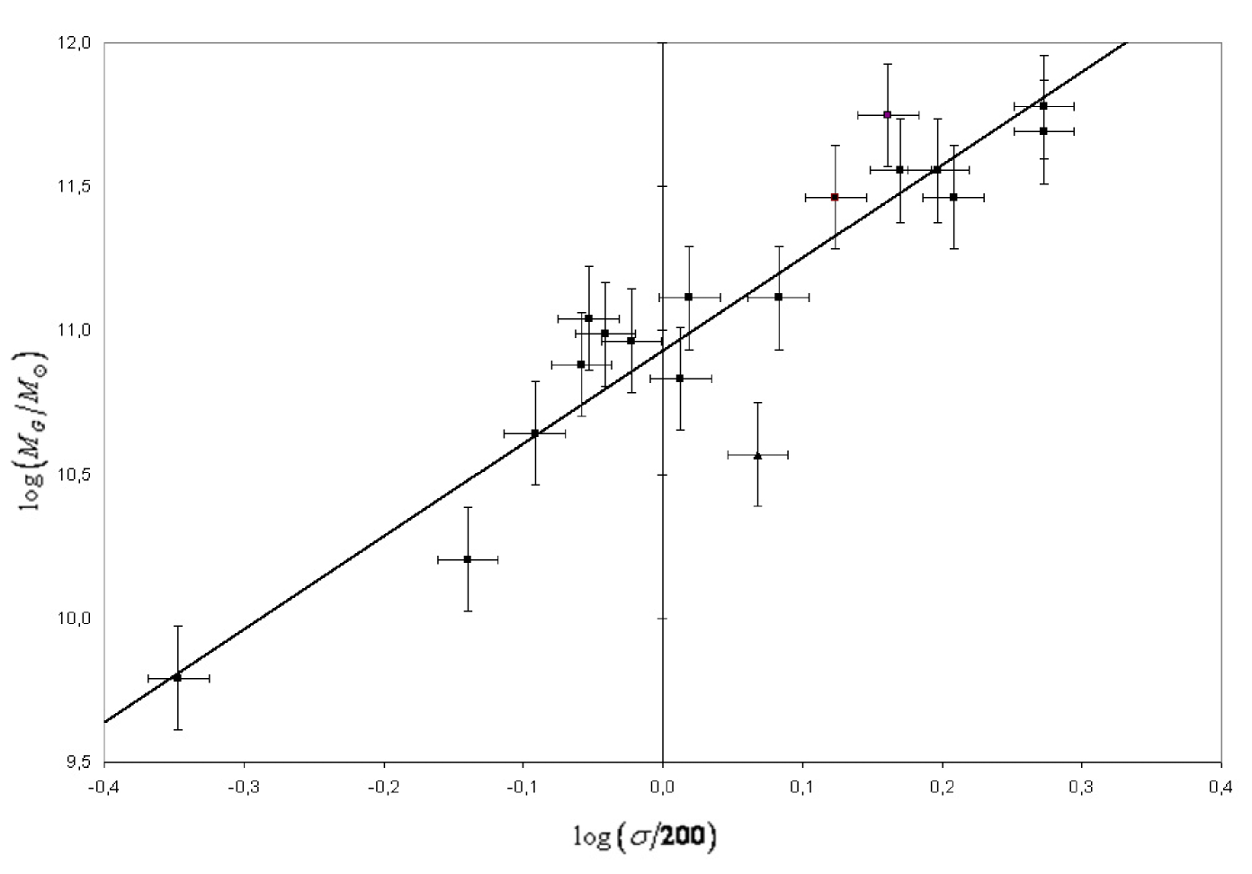
Figure 2: The mass of the galaxy $M_{G}$ versus $\sigma/200$ of the host elliptical galaxy. The solid line is the best fit (14) with Fitexy Routine. The error bars are such that $\Delta LogM_{G}=0.18$ and $\sigma$ has a relative error of $5\%$. We denote with a triangle the galaxy NGC5845 with the largest residual.

This result cannot be explained with the Faber - Jackson relation while it could be in agreement with the $L\propto\sigma^{2}$ or $L\propto\sigma^{2.5}$ obtained for faint ellipticals [23, 24]. The very interesting fit of equation (14) is shown in Fig. 2 where it is evident that the galaxy N5845 (denoted by a triangle) has the largest residual. Eliminating this galaxy, the best fit line (14) does not change while the linear correlation coefficient increases becoming $r_{C}=0.958$ and the value of $\chi^{2}$ decreases from 20.07 to 10.55 resulting in a very strong correlation.

While a coefficient less than one as $0.8$ is more difficult to be interpreted, it would be more interesting, from the theoretical point of view, the meaningful possibility of an exact linear relationship between the mass of a SMBH and the kinetic energy of random motions of the host galaxy. It is very simple to test this hypothesis using the exact formulas (without any approximation or iterative procedure) of the standard ”least-squares method” that we have reported in the appendix.

(1)	(2)	(3)	(4)	(5)
Sample	N	m	$b\pm\Delta b$	$\chi^{2}$
$A$	13	1	$3.73\pm 0.08$	23.67
$B$	11	1	$3.86\pm 0.09$	11.54
$A^{\prime}$	13	1	$3.56\pm 0.08$	28.31
$B^{\prime}$	11	1	$3.59\pm 0.09$	23.19
$C$	18	1	$3.52\pm 0.07$	37.91
$D$	29	1	$3.58\pm 0.06$	58.20

Table 5: We denote in column (1) the sample, in column (2) the corresponding number of galaxies, in column (3) we fix the coefficient $m=1$ and we find with Fitexy the best fit of the relationship $\log(M_{BH})=m\cdot\log(M_{G}\sigma^{2}/c^{2})+b$. The result for $b$ is in column (4) and the corresponding $\chi^{2}$ in column (5).

The results are listed in Table 5 and we argue that for the sample B the hypothesis is certainly right, and for the samples A and $B^{\prime}$ it can be acceptable. Only the samples $A^{\prime}$ and C have a too high $\chi^{2}$. The linear fit of sample C is shown in fig. 1 with a dashed line and involves $M_{BH}c^{2}\propto M_{G}\sigma^{2}$.

The fourth test for our relationship is the inclusion of lenticular and spiral galaxies in the statistical analysis. Our sample D is now composed by all the 29 galaxies listed in Table 2. In Fig. 3 we show with a dashed line the best fit (11) for the 18 ellipticals (denoted with boxes), with the dot - dashed line the best fit for the remaining 11 galaxies (denoted with circles):

$$Log(M_{BH})=(1.14\pm 0.15)Log\frac{M_{G}\sigma^{2}}{c^{2}}+(3.14\pm 0.57)$$

and with a solid line the best fit for the whole sample D

$$Log(M_{BH})=(0.90\pm 0.05)Log\frac{M_{G}\sigma^{2}}{c^{2}}+(4.03\pm 0.24)$$

We argue that the contribution of lenticular and spiral galaxies increases the slope that becomes closer to unity.

4 Conclusions

From the first samples of data (A and B) we were induced in a previous paper [16] to consider a relationship between the masses of SMBHs and the kinetic energy of random motions in elliptical galaxies. This suggestion is now confirmed first by reanalyzing the old data using the Fitexy Routine and then comparing the results with the corresponding fit of a new set of kinematical data extracted from the paper of Häring and Rix [8]. In the light of Fig. 3 we show that the relationship works well also for lenticular and spiral galaxies. The remarkable result is that the relationship we proposed (7), has now a smaller scatter with respect to the old equation (6) and the $M_{BH}$ vs $M_{G}$ law. Furthermore we have shown that, using the new data, all these relationships can be strictly connected because (unlike AFDM) the mass of the galaxy strongly depends on the velocity dispersion: the linear correlation coefficient of this relationship (8) is very high and the $\chi^{2}$ very low. Finally our result (14) with $\gamma=3.2$ is surprisingly smaller than the ones expected of $\gamma=4$ or $\gamma=5$.

For the sample A and B, given the assumptions of the model of Busarello, Longo and Feoli [17], it is clear that triaxiality, anisotropy of the velocity field, inclination, deviations from the $r^{1/4}$ law, are all sources of possible errors that could affect the derived kinematical parameters. For the remaining samples we must consider that the masses are not computed with the same method and often refer to a bulge region that ends to $r_{MAX}=3R_{e}$. At the same time all the velocity dispersions are no longer averaged until the effective semimajor axis of each galaxy. So the nonhomogeneity of the measurements and the differences in the part of the galaxy that each single measure now considers, can affect also the results obtained with the new set of data. Of course a rigorous analysis will be possible only when the observational uncertainties in all quantities are reduced and the sample is further extended. However, though with the caution due to all these possible error sources, the study of the relationship we propose between the rest energy of a SMBH and the kinetic energy of random motions of the host galaxy appears to be very useful for a more complete understanding of the formation and evolution of SMBH not only in elliptical galaxies.

Acknowledgements

We are grateful to Gaetano Scarpetta, Antonio D’Onofrio and Nicola De Cesare for useful comments and Franco Caprio for helpful suggestions about computer programs. The research was partially supported by FAR fund of the University of Sannio.

Appendix

We have tried to maximize the errors so we have always chosen in the Table 1 of Tremaine et al.[3] the maximal difference between the measure of the black hole mass and its high or low values in parenthesis. So, for example, for NGC 3379 the measure $M_{BH}=1.0\times 10^{8}(0.5,1.6)$ becomes in our statistical elaboration (see column 2 of Table 2) $M_{BH}=(1.0\pm 0.6)\times 10^{8}$.

Accordingly, the formula used in this paper to estimate all the maximal errors in the functions F of the parameters $(a,b,c,....)$ is

$$\Delta F(a,b,c)=\left|\frac{\partial F}{\partial a}\right|\Delta a+\left|\frac{\partial F}{\partial b}\right|\Delta b+\left|\frac{\partial F}{\partial c}\right|\Delta c$$

Furthermore the reduced $\chi^{2}$ is defined as:

$$\chi^{2}_{r}=\frac{\chi^{2}}{N-1}=\frac{1}{N-1}\sum_{i=1}^{N}\frac{(y_{i}-b-mx_{i})^{2}}{(\Delta y_{i})^{2}+m^{2}(\Delta x_{i})^{2}}$$

for a relation of the form $y=b+mx$.

In the case $m=1$ we have used the exact formulas of the least squares method:

$$b=\frac{\sum_{i=1}^{N}\left(\frac{y_{i}-x_{i}}{(\Delta x_{i})^{2}+(\Delta y_{i})^{2}}\right)}{\sum_{i=1}^{N}\left(\frac{1}{(\Delta x_{i})^{2}+(\Delta y_{i})^{2}}\right)}$$

$$(\Delta b)^{2}=\frac{1}{\sum_{i=1}^{N}\left(\frac{1}{(\Delta x_{i})^{2}+(\Delta y_{i})^{2}}\right)}$$

and the results are reported in Table 5.

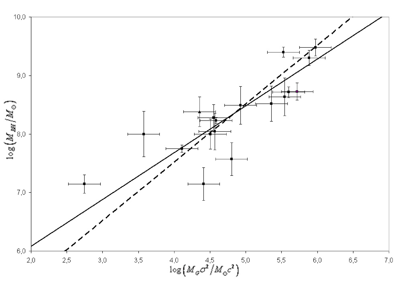
Figure 1: SMBH mass versus $M_{G}\sigma^{2}/c^{2}$ of the host elliptical galaxy. The solid line is the best fit (11) with Fitexy Routine, the dashed line is the best linear fit ($m=1$, $b=3.55\pm 0.07$) with the exact formulas of the least squares method (see appendix, eqs. A3 and A4). The error bars for $M_{BH}$ are from [3] and we assume $\Delta LogM_{G}=0.18$ and for $\sigma$ a relative error of $5\%$

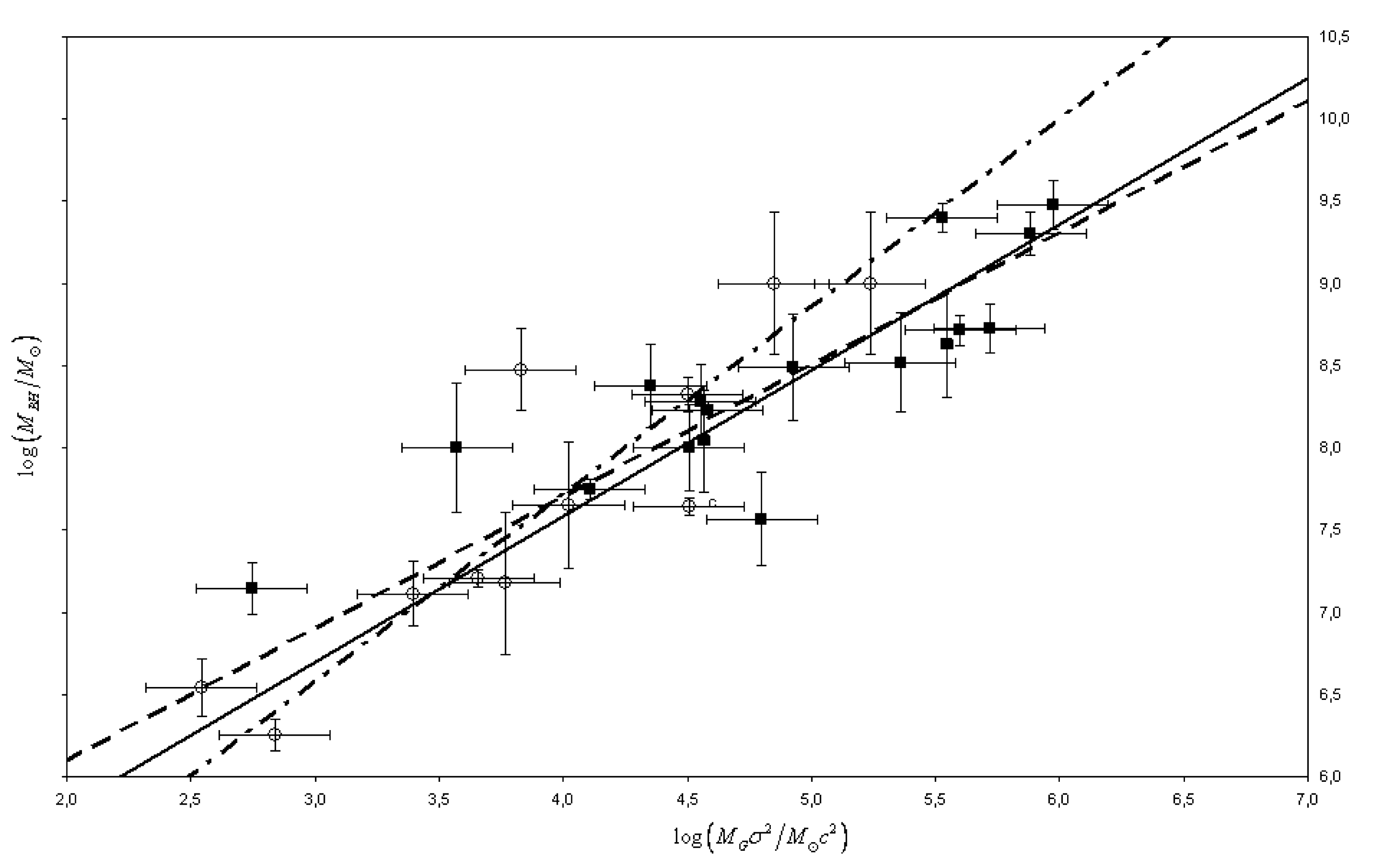
Figure 3: SMBH mass versus $M_{G}\sigma^{2}/c^{2}$ of the host galaxy. The dashed line is the best fit (11) with Fitexy Routine for the 18 ellipticals denoted with boxes, the dot - dashed line is the best fit (15) for the remaining 11 lenticular and spiral galaxies denoted with circles. Finally the solid line is the best fit (16) for the whole sample D of 29 galaxies. The error bars for $M_{BH}$ are from [3] and we assume $\Delta LogM_{G}=0.18$ and for $\sigma$ a relative error of $5\%$

References

- [1] L. Ferrarese and D. Merritt, Astrophysical Journal 539, L9 (2000).
- [2] K. Gebhardt et al., Astrophysical Journal Letter 539, 13 (2000).
- [3] S. Tremaine et al., Astrophysical Journal 574, 740 (2002).
- [4] J. Kormendy and D. Richstone Annual Review of Astronomy and Astrophysics33, 581 (1995);
- [5] J. Magorrian et al., Astronomical Journal 115, 2285 (1998);
- [6] A. Marconi et al., in IAU Symp. 205, Galaxies and their Constituents at the Highest Angular Resolutions, ed. R. T. Schilizzi, S. Vogel, F. Paresce and M. Elvis, (S.Francisco: Astronomical Society of the Pacific.), 58, (2001)
- [7] D. Merritt and L. Ferrarese, in APS Conf. Ser. 249, The Central kpc of Starbursts and AGN, ed. J. H. Knapen, J.E. Beckman, I. Shlosman and T.J. Mahoney, (San Francisco: Astronomical Society of the Pacific), 335, (2001)
- [8] N. Häring and H. Rix, Astrophysical Journal Letter, 604, L89, (2004)
- [9] D. Richstone et al., Nature, 395, A14, (1998)
- [10] R. P. Van der Marel, in IAU Symp. 186, Galaxy interactions at Low and High Redshift, ed. D. B. Sanders and J. Barnes, (Dordrecht: Kluwer Academic Publishers), (2002)
- [11] L. Ferrarese, Astrophysical Journal, 578, 90, (2002)
- [12] A. Burkert and J. Silk, Astrophysical Journal, 554, L151, (2001)
- [13] V. I. Dokuchaev and Yu. N. Eroshenko, preprint (astro-ph/0209324), (2002)
- [14] M. G. Haehnelt and G. Kauffmann, Monthly Notices of the Royal Astronomical Society, 318, L35, (2000)
- [15] F. C. Adams, D. S. Graff and D. O. Richstone, Astrophysical Journal, 551, L31, (2000)
- [16] A. Feoli and D. Mele, International Journal of Moden Physics D, 14, 1861, (2005)
- [17] G. Busarello, G. Longo and A. Feoli, Astronomy and Astrophys., 262, 52, (1992)
- [18] G. Busarello and G. Longo, Morphological and Physical Classification of Galaxies, eds. G. Longo et al. (Dordrecht: Kluwer Academic Publishers), 423, (1992)
- [19] A. Curir, F. De Felice, G. Busarello and G. Longo, Astrophys. Letter Commun., 28, 323, (1993)
- [20] Orear, J. 1982, American Journal of Physics, 50, 912, (1982)
- [21] M. G. Akritas and M. A. Bershadi, Astrophysical Journal, 470, 706, (1996)
- [22] G. de Vaucouleurs et al., Third Reference Catalogue of Bright Galaxies, (Berlin Heidelberg New York: Springer - Verlag), (1991)
- [23] R. L. Davies, G. Efstathiou, M. Fall, G. Illingworth and R. L. Schechter, Astronomical Journal, 266, 41, (1983)
- [24] A. Matković and R. Guzmán, Monthly Notices of the Royal Astronomical Society, 362, 289, (2005) and references therein.