Quasar Proximity Zones and Patchy Reionization

Abstract

Lyman-alpha (Ly$\alpha$) forest absorption spectra towards quasars at $z\sim 6$ show regions of enhanced transmission close to their source. Several authors have argued that the apparently small sizes of these regions indicate that quasar ionization fronts at $z\gtrsim 6$ expand into a largely or partly neutral intergalactic medium (IGM). Assuming that the typical region in the IGM is reionized by $z\leq 6$, as is suggested by Ly$\alpha$ forest observations, we argue that at least $50\%$ of the volume of the IGM was reionized before the highest redshift quasars turned on. Further, even if the IGM is as much as $\sim 50\%$ neutral at quasar turn-on, the quasars are likely born into large galaxy-generated HII regions. The HII regions during reionization are themselves clustered, and using radiative transfer simulations, we find that long skewers through the IGM towards quasar progenitor halos pass entirely through ionized bubbles, even when the IGM is half neutral. These effects have been neglected in most previous analyses of quasar proximity zones, which assumed a spatially uniform neutral fraction. We model the subsequent ionization from a quasar, and construct mock Ly$\alpha$ forest spectra. Our mock absorption spectra are more sensitive to the level of small-scale structure in the IGM than to the volume-averaged neutral fraction, and suggest that existing proximity-zone size measurements are compatible with a fully ionized IGM. However, we mention several improvements in our modeling that are necessary to make more definitive conclusions.

1. Introduction

The Epoch of Reionization (EoR), when HII regions grow around galaxies and/or quasars, eventually overlap and fill the entire IGM, is fundamental to our understanding of cosmological structure formation. Detailed observations of the EoR will characterize the nature of the first luminous sources in the Universe, describe their impact on the surrounding IGM, and fill in a significant gap in our knowledge of the history of the Universe. Prospects for observational advances are bright: 21cm observations (e.g. Madau et al. 1997, Zaldarriaga et al. 2004, for a review see Furlanetto et al. 2006a), improved measurements of polarization of the cosmic microwave background (CMB) (Zaldarriaga 1997, Kaplinghat et al. 2003), small-scale CMB fluctuations (e.g. Zahn et al. 2005, McQuinn et al. 2005), increasingly deep narrow-band Ly-$\alpha$ surveys (e.g. Haiman & Spaans 1999, Barton et al. 2004, Furlanetto 2006b, McQuinn et al. in prep.), optical afterglow spectra of gamma ray bursts (GRBs) (Barkana & Loeb 2004), quasar absorption spectra (Fan et al. 2006), and other probes, promise a wealth of new data in the near future.

What have we learned from existing observations? This is, of course, an intrinsically interesting question, but it is also an important one for directing the design of future surveys and experiments. For example, current constraints can provide important guidance regarding the optimal target redshift range for future reionization surveys.

Inferences about the duration of the EoR come from measurements of anisotropies in the polarization of the CMB (Page et al. 2006), narrow-band surveys for Ly-$\alpha$ emitters (e.g. Malhotra & Rhoads 2005), the optical afterglow of a $z=6.3$ GRB (Totani et al. 2006), and particularly the absorption spectra of high redshift quasars (e.g. Fan et al. 2006). While valuable and exciting, these observations have yielded constraints on the EoR that are generally weak and subtle to interpret. The central value for the electron scattering optical depth from WMAP favors reionization activity at $z\gtrsim 11$, but, at the $1-\sigma$ level, current limits are consistent with rapid reionization ending near $z\sim 6$ (Page et al. 2006). Indeed, at $\sim 3-\sigma$ the data are consistent with no reionization whatsoever (Page et al. 2006).

Malhotra & Rhoads (2005) have constrained the ionized volume fraction in the IGM by counting the abundance of Ly-$\alpha$ emitters at $z=6.5$, and requiring a minimum ionized volume around the sources to avoid attenuating their Ly-$\alpha$ photons. In this manner, Malhotra & Rhoads quote an upper limit on the neutral volume fraction of the IGM, $X_{\rm HI}\lesssim 0.5$. In reality, the sources likely reside in much larger ionized regions (e.g. Furlanetto et al. 2006b), and this constraint should be tightened with more detailed modeling. For example, Dijkstra at al. (2006) find that these observations imply $X_{\rm HI}\lesssim 0.2$.

The optical afterglow spectra of $z\gtrsim 6$ GRBs can, in principle, be used to search for damping-wing absorption redward of Ly-$\alpha$, a signature of a largely neutral IGM (Miralda-Escudé 1998, Barkana & Loeb 2004). However, most GRB optical afterglows show evidence for damped Lyman-alpha absorbers associated with their host galaxies, which are problematic to distinguish from a largely neutral IGM (Totani et al. 2006). Even so, Totani et al. (2006) use the Ly-$\beta$ region of a $z=6.3$ afterglow to argue against a largely neutral IGM, giving a constraint of $X_{\rm HI}\lesssim 0.6$.

Presently, the most detailed information on the state of the IGM at $z\sim 6$ comes from Ly-$\alpha$ forest absorption towards high redshift quasars (e.g. Fan et al. 2006). It is difficult to derive constraints on the ionization state of the IGM from the spectra of these quasars, owing to the large absorption cross section for Ly-$\alpha$ photons. Indeed, a highly ionized IGM ($X_{\rm HI}\gtrsim 10^{-4}$) results in complete absorption in a $z\sim 6$ Ly-$\alpha$ forest spectrum (Gunn & Peterson 1965). In spite of this intrinsic complication, a little ingenuity has led to substantial progress.

For example, one can measure absorption in the Ly-$\beta$ and Ly-$\gamma$ troughs of a quasar spectrum. Owing to their weaker absorption cross sections, when these transitions are saturated they imply tighter constraints on the ionization state of the IGM than the optical depth in Ly-$\alpha$. This approach has been used to suggest that the IGM is evolving rapidly near $z\sim 6$ (e.g. Fan et al. 2002, Cen & McDonald 2002, Lidz et al. 2002, Fan et al. 2006). The constraints are, however, consistent with a mostly ionized IGM. Furthermore, the transmission is influenced strongly by rare underdense regions at high redshift, and so the conclusions depend sensitively on the probability distribution of gas in the IGM (Oh & Furlanetto 2005, Becker et al. 2006a). Another interesting statistic is to consider how much the absorption, averaged over large stretches of spectra, varies from sightline-to-sightline. Close to and during reionization, the ultraviolet radiation background should fluctuate strongly (e.g. Zuo 1992, Wyithe & Loeb 2005a) and potentially increase the sightline-to-sightline scatter in the mean absorption. However, current measurements are broadly consistent with density fluctuations alone (Lidz et al. 2006a, Liu et al. 2006).

It is also possible to use a metal line tracer of the ionization state of the IGM, such as OI, which conveniently lies redward of Ly-$\alpha$ and has an ionization potential similar to that of hydrogen (Oh 2002). In fact, high-resolution Keck spectra of the $z\sim 6$ SDSS quasars do reveal some OI lines, with $4$ out of $6$ detected systems lying towards the highest redshift quasar known (Becker et al. 2006b). Interestingly, some of the OI systems are nearby regions that show transmission in the Ly$\alpha$ and Ly$\beta$ forests of this quasar (Becker et al. 2006b). The interpretation of these observations is unclear: the OI systems might reflect dense clumps of neutral gas in a highly ionized IGM, or instead could indicate inhomogeneous metal pollution in a more neutral IGM.

Finally, the tightest constraints claimed on the ionization state of the $z\sim 6$ IGM come from measurements of the proximity regions around $z\sim 6$ quasars. Several authors, starting with Wyithe & Loeb (2004), have argued that these regions are small, indicating that quasar ionization fronts are expanding into a largely neutral IGM. Mesinger & Haiman (2004) claim to detect the edge of a quasar ionization front around one of the SDSS $z\sim 6$ quasars, using additional leverage from the Ly$\beta$ region, and suggest that the neutral fraction is $X_{\rm HI}\gtrsim 0.25$ at $z\sim 6$. These authors’ constraint comes not so much from the apparent size of the proximity zone, but from the detailed radial dependence of the transmission and from a stretch of spectrum with Ly$\beta$ transmission and no corresponding Ly$\alpha$ transmission. They attribute this to damping wing absorption, a signature of a partly neutral IGM. Oh & Furlanetto (2005), however, argue that such stretches occur at high redshift even when the IGM is highly ionized and may not indicate damping wing absorption. Fan et al. (2006) emphasize caution in interpreting proximity region measurements, but observe rapid evolution in the sizes of quasar proximity regions from $z=5.7-6.3$, arguing for a correspondingly rapid evolution in the neutral fraction. Their final constraint is based on only the evolution of the proximity region size, which they argue reflects the change in the neutral fraction. Consequently, they quote a significantly more conservative limit than previous authors, requiring a volume-weighted neutral fraction of only $X_{\rm HI}\gtrsim 10^{-3}$.

Recently, more detailed proximity zone calculations have been performed. Bolton & Haehnelt (2006) studied quasar transmission carefully using 1D radiative transfer calculations, and determined that it is difficult in general to distinguish highly ionized and mostly neutral models with proximity zone measurements. Maselli et al. (2006) came to a similar conclusion. Mesinger & Haiman (2006), however, argue that detailed fitting of the transmission pdf in the quasar proximity zones favors a partly neutral IGM, with a lower limit of $x_{\rm HI}\gtrsim 0.033$, and a considerably larger preferred value.

In each of these studies, the authors have assumed that quasar ionization fronts expand into a uniformly ionized surrounding IGM, with some low level, yet homogeneous background ionization. If the $z\gtrsim 6$ quasar spectra truly probe the pre-reionization epoch, then this is likely a very poor approximation. The pre-reionization IGM should resemble swiss cheese (Loeb 2006), with large HII regions forming around clustered galaxies embedded in a surrounding neutral IGM (e.g. Sokasian et al. 2003, Ciardi et al. 2003, Furlanetto et al. 2004a,c, Iliev et al. 2006, Zahn et al. 2006, McQuinn et al. 2006a, Trac & Cen 2006). Naively, this complicates distinguishing partly neutral and highly ionized models on the basis of quasar proximity zones. Quasar ionization fronts may extend further along sightlines that traverse several ionized HII regions, and be more limited along other directions that traverse several neutral patches. Moreover, transmission at the edge of the proximity zone may be related to background galaxies rather than the quasar itself, making it still harder to locate the ‘edge’ of the proximity zone using absorption spectra (see also Wyithe & Loeb 2006a). Our present paper extends these earlier works, and focuses on how ‘patchy reionization’ impacts quasar proximity zones.

The outline of our paper and our basic line of argument is as follows. Given that most of the volume of the IGM appears to be highly ionized by $z\lesssim 6$, we argue that reionization is unlikely rapid enough for the IGM to be mostly neutral when the highest redshift quasars observed turned on (§2). From these considerations, we suggest that the IGM is at least $50\%$ ionized at quasar turn-on. In §3, we describe 3D radiative transfer calculations for plausible partly neutral models, detailing the initial ionization state of the IGM. Here we argue that the highest redshift quasars are born into large HII regions, even if as much as $50\%$ of the volume of the IGM is neutral. Yu & Lu (2005) previously argued that overdense $z\sim 6$ quasar environments should reionize before typical regions, but here we examine the consequences of this in more detail, and arrive ultimately at somewhat different conclusions. Even in this maximally ($50\%$) neutral scenario, we find long skewers towards quasar progenitor halos which pass entirely, or predominantly, through ionized bubbles.

Using the initial ionization field from our 3D calculations as input, we perform (more detailed) 1D radiative transfer calculations, describing the subsequent propagation of quasar ionization fronts (§4). Here we find that quasar front extents, in our patchy reionization models, depend sensitively on the long ionized pathways created by surrounding galaxies before the quasar is born. Since quasars are typically born into large HII regions, the fronts tend to extend further in patchy reionization models than in models with a uniform IGM of the same neutral fraction, although with significant sightline-to-sightline variation. In §5 we construct mock absorption spectra and show, in agreement with previous authors (Bolton & Haehnelt 2006, Maselli et al. 2006), that it is difficult to accurately recover the position of a quasar front, and that estimates of the front position from absorption spectra are generally underestimates. This is a consequence of the typically high Ly$\alpha$ opacity at the edge of a $z\sim 6$ quasar front. We suggest, however, an alternative algorithm for finding front positions from absorption spectra. We then estimate the importance of unresolved (in our numerical simulations) small scale structure on our mock absorption spectra. Our results are more sensitive to the highly uncertain level of small scale structure in the IGM than to the volume-weighted ionization fraction. Finally, in §6 we conclude and discuss possible future research directions.

Throughout, we assume a flat, $\Lambda$CDM cosmology parameterized by: $\Omega_{m}=0.3$, $\Omega_{\Lambda}=0.7$, $\Omega_{b}=0.04$, $H_{0}=100h$ km/s/Mpc with $h=0.7$, and a scale-invariant primordial power spectrum with $n=1$, normalized to $\sigma_{8}(z=0)=0.9$. Our adopted value for $\sigma_{8}$ is a little larger than the central value favored by $3$-year constraints from WMAP (Spergel et al. 2006), but uncertainties in the cosmological model are sub-dominant to other aspects of our theoretical modeling, which we detail subsequently.

2. Initial Conditions

Now, we consider the question: what should we expect for the ionization state of the gas around $z\gtrsim 6$ quasars when they turn on? In this section, we address this issue using a rough analytic model; in the subsequent section we describe 3D radiative transfer calculations which examine this in more detail.

First, recall that constraints from $z\lesssim 6$ quasar spectra suggest that the IGM is highly ionized by $z\lesssim 6$ (e.g. Fan et al. 2002), although see §6 for a critical discussion. To date, the highest redshift quasar observed is at $z_{q}=6.42$. If this source turns on over roughly a Salpeter time ($t_{s}\sim 4\times 10^{7}$ yrs) before being observed, then its turn-on redshift is $z_{\rm on}\sim 6.66$. For the surrounding IGM to be mostly neutral at quasar birth, yet highly ionized by $z\lesssim 6$, reionization must proceed extremely rapidly, occurring over a short redshift span of $\Delta z\lesssim 0.7$ or $\sim 10^{8}$ yrs. Obviously, reionization must occur even more rapidly if measurements truly indicate that other quasars at slightly lower redshifts with $z_{q}\gtrsim 6$, (e.g. the $z_{q}=6.28$ quasar SDSS J1030+0524), are also born when the surrounding IGM is highly neutral.

Second, the $z\gtrsim 6$ quasars are thought to reside in very rare and massive host halos (Fan et al. 2001, Li et al. 2006), and hence the surrounding IGM is likely overdense out to large scales around the quasars (Loeb & Eisenstein 1995, Barkana 2004, Faucher-Giguère et al. 2007). These regions should reionize before typical ones since halo collapse and galaxy formation are expected to occur earlier in large-scale overdensities (e.g. Barkana & Loeb 2004). The abundance of ionizing sources in an overdense region at a given time should resemble the abundance of sources in a typical region at a later time. Even if typical regions in the IGM are neutral when quasars turn on, the same may not be true of the overdense environments where quasars reside (see also Yu & Lu 2005). Recombinations are also more efficient in overdense regions – this could offset the tendency for overdensities to reionize first, but this is unlikely to remove the trend. This is because galaxy formation is more sensitive to large scale overdensity than the recombination rate – indeed, the abundance of high mass halos is exponentially sensitive to the large scale overdensity (Barkana & Loeb 2004, Furlanetto & Oh 2005, Wyithe & Loeb 2006b).

2.1. Globally-Averaged Ionization Fractions

In this section we illustrate these effects using simple analytic estimates. We perform these calculations with the analytic model of Furlanetto et al. (2004). In its simplest incarnation, this method assumes that a galaxy of mass $M_{\rm gal}$ can ionize a surrounding mass in the IGM of $M_{\rm ion}=\zeta M_{\rm gal}$. With this assumption, one can show that the average ionization fraction of gas in a region of radius $R$ and linear overdensity $\delta_{R}$ is given by:

$$\langle x_{i}|\delta_{R},R\rangle=\zeta(f_{\rm coll}|M_{\rm min},R,\delta_{R}).$$ (1)

Here, $(f_{\rm coll}|M_{\rm min},R,\delta_{R})$ is the fraction of mass in halos with mass larger than $M_{\rm min}$ in a region of over-density $\delta_{R}$ and radius $R$. In this equation, the impact of recombinations is absorbed into the parameter $\zeta$. For our simple estimates below we hence ignore the recombination-rate enhancement in over-dense regions.

The collapse fraction in an overdense region is given by:

$$(f_{\rm coll}|M_{\rm min},\delta_{c},M,\delta_{M})=\rm{erfc}\left[\frac{\delta_{c}-\delta_{M}}{\sqrt{2\sigma^{2}_{\rm min}-2\sigma^{2}_{M}}}\right]\,,$$ (2)

where $\delta_{c}$ is the critical overdensity for collapse, $M$ indicates the mass scale corresponding to the spatial scale $R$, and $\sigma^{2}_{\rm min}$ and $\sigma^{2}_{M}$ are the variance of the linear density field smoothed on mass scales $M_{\rm min}$ and $M$, respectively. The global collapse fraction follows from this expression in the limit $\delta_{M}\rightarrow 0$, $\sigma^{2}_{M}\rightarrow 0$. This equation implies that overdense regions will have larger collapse fractions than regions at the mean density and, under the assumptions of Equation (1), will be ionized earlier.

Consder, first, the redshift evolution of the globally-averaged ionization fraction, by taking $\delta_{R}\rightarrow 0$ and $R\rightarrow\infty$ in Equation (1). The precise duration of reionization depends sensitively on the nature of the sources producing ionizing photons at early times, which is highly uncertain. If rare, yet efficient sources reionize the IGM then the collapse and ionization fractions should grow rapidly with redshift (Equations 1 and 2). Furthermore, the duration of the reionization epoch depends on the efficiency of thermal feedback, the time taken to photo-evaporate mini-halos in the IGM, as well as the detailed properties and evolution of the cosmic star-formation rate and the fraction of ionizing photons escaping into the IGM. In our model, all of these details are subsumed into a single, redshift-independent parameter, $\zeta$ (Equation 1).

Nevertheless, we can roughly gauge the range of possibilities by varying the parameter $M_{\rm min}$ in Equation (2), in each case normalizing $\zeta$ to match $\langle x_{i}\rangle=1$ at $z=6$. Of course, reionization may finish at significantly higher redshift (i.e., $\langle x_{i}\rangle=1$ is reached at $z>6$); our goal here is to find the maximally neutral case at quasar turn-on provided that the entire volume is reionized by $z\lesssim 6$. We consider a wide range of values for $M_{\rm min}$. On the low end, we adopt $M_{\rm min}=M_{\rm cool}$, and on the high end we take $M_{\rm min}=10^{3}M_{\rm cool}$. Here, $M_{\rm cool}$ denotes the dark matter halo mass corresponding to a virial temperature of $10^{4}$ K ($M_{\rm cool}=1.3\times 10^{8}M_{\odot}$ at $z\sim 7$, e.g. Barkana & Loeb 2001), above which atomic line cooling is efficient, allowing gas to cool, condense to form stars, and produce ionizing photons. The higher minimum source mass scenarios approximate models where photo-heating has limited the efficiency of star-formation in small mass halos (Thoul & Weinberg 1996, Navarro & Steinmetz 1997, Dijkstra et al. 2004), and models in which supernova winds suppress star-formation in low mass halos (e.g. Springel & Hernquist 2003). We note that our highest minimum source mass model ($M_{\rm min}=10^{3}M_{\rm cool}$) is rather extreme, considerably larger than the suppression masses suggested by the above studies. We consider this case anyway to illustrate a plausible upper limit.

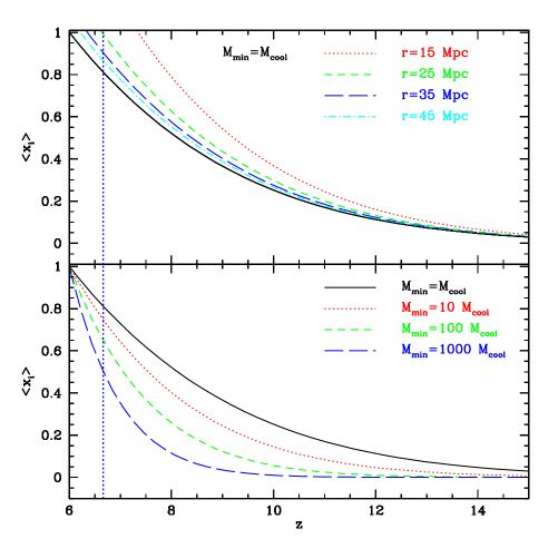
Figure 1.— Redshift evolution of the volume-averaged ionization fraction. Top panel: The black solid line shows the redshift evolution of the ionization fraction in a typical region of the IGM, with the ionizing source efficiency calibrated so that $\langle x_{i}\rangle=1$ at $z=6$, assuming all halos down to $M_{\rm cool}$ contribute ionizing photons with equal efficiency. The other curves indicate the average ionization fraction in spherical regions of different size, each with a massive quasar host (here $M_{\rm dm,host}=10^{13}M_{\odot}$) at the center. The vertical blue dotted line indicates a plausible turn-on time for a $z=6.42$ quasar. The curves illustrate that: i) the process of reionization takes a sufficiently long time that, even if it completes at $z=6$, the typical location in the IGM is already $\sim 80\%$ ionized (in this model) when the $z=6.42$ quasar turned on; and ii) provided that quasar host halos reside in highly overdense regions, their surroundings will reionize earlier than the typical region in the IGM. Bottom panel: The redshift evolution of the volume-averaged ionization fraction for a typical region as a function of the minimum host halo mass. If rare, very efficient, sources produce most of the ionizing photons, reionization occurs more rapidly than if highly abundant yet less efficient sources produce most of the ionizing photons. In each model, more than $50\%$ of the IGM volume is ionized at quasar turn-on.

We show the redshift evolution of the globally-averaged ionization fraction in the bottom panel of Figure 1. The first qualitative feature apparent from the Figure is that reionization is generally quite extended: for example, in the cooling mass model the average ionization fraction is $\langle x_{i}\rangle=0.1,0.5,0.7,1.$ at $z\sim 12,8,7$, and $z\sim 6$ respectively. If the highest redshift quasar observed thus far, at $z_{q}=6.42$, turns on at $z_{\rm on}\sim 6.66$ as motivated above, the average ionization fraction in this model is $\sim 80\%$ at turn-on. The process is less extended if the sources are rare, yet very efficient. For example, in the $M_{\rm min}=10^{2}M_{\rm cool}$ case, the IGM is only $\sim 60\%$ ionized at quasar turn on. However, even in the very extreme $M_{\rm min}=10^{3}M_{\rm cool}$ scenario, $50\%$ of the IGM is ionized by quasar turn on at $z\sim 6.66$. The ionization fraction evolves more rapidly in the high minimum mass models, since here the host halos are still on the exponential tail of the mass-function near $z\sim 6$, and hence their abundance evolves quickly with redshift. Note that we likely over-estimate this effect, since we use Press-Schechter (1974) theory for simplicity: the halo abundance from recent high redshift numerical simulations more closely matches the Sheth-Tormen (1999) mass function, indicating that Press-Schechter theory underestimates the abundance of rare halos (Reed et al. 2003, Heitmann et al. 2006, Zahn et al. 2006, Lukic et al. 2007, although see Trac & Cen 2006). Note that although our constraint argues that the IGM is at least somewhat ionized when the highest redshift quasar observed turns on, it is not in conflict with the formal limits from Wyithe & Loeb (2004), Wyithe et al. (2005a), and Mesinger & Haiman (2004, 2006).

Furthermore, we have taken $\zeta$ as a free parameter, simply fixing it to match $\langle x_{i}\rangle=1$ at $z\sim 6$. In fact, if all of the ionizing photons are indeed produced by the very rare halos with $M\gtrsim M_{\rm min}=10^{3}M_{\rm cool}$, the sources need to be exceedingly efficient to reionize the IGM by $z\lesssim 6$. Specifically, we estimate the number of ionizing photons per stellar baryon required in this model to achieve $\langle x_{i}\rangle=1$ by $z=6$, using Equations (82) and (83) of Furlanetto et al. (2006a). We adopt typical values of three recombinations per ionized hydrogen atom, an escape fraction of $f_{\rm esc}=0.1$, and a star-formation efficiency of $f_{\star}=0.1$, and find that $N_{\gamma}\sim 70,000$ ionizing photons per baryon are required in this scenario. This ionizing efficiency is substantially larger than the value expected for a Salpeter IMF, $N_{\gamma}\sim 4,000$ (e.g. Cohn & Chang 2006), although it is achievable if the IMF is very top-heavy (e.g. Bromm et al. 2001) even at $z\sim 7$ in spite of apparently wide-spread metal enrichment by $z\sim 6$ (Ryan-Weber et al. 2006).

Finally, in §6 we argue that it is conceivable that $\langle x_{i}\rangle=1$ is achieved later than $z=6$ – reionization might end at as low a redshift as $z\sim 5.5$. Even if reionization completes only by $z=5.5$ we find that the neutral fraction at quasar turn-on is less than $50\%$ in all of our models except our extreme $M_{\rm min}=10^{3}M_{\rm cool}$ model. Moreover, reionization is likely more extended than in our model – for example, thermal feedback and mini-halos can extend the duration of reionization compared to our simple predictions (e.g. Haiman & Holder 2003, McQuinn et al. 2006a). Therefore, our simple estimates indicate that the IGM is unlikely as much as $50\%$ neutral at quasar turn-on and is more likely at least $70\%$ ionized by this time. These rough estimates are inevitably model dependent, but are in accord with observational constraints from Ly$\alpha$ emitters (Malhotra & Rhoads 2005, Haiman & Cen 2005, Dijkstra et al. 2006), and GRB optical afterglow spectra (Totani et al. 2006) which coincidentally give similar upper limits for the neutral fraction near the plausible turn-on redshifts of the $z\gtrsim 6$ quasars.

2.2. The Ionization Field Around Quasar Progenitor Halos

The above calculations apply to typical regions in the IGM. We now extend our analysis to consider the ionization of the overdense environments expected around high redshift quasars. We will compute the probability distribution of the ionized fraction spherically-averaged around plausible quasar host halos, prior to quasar turn-on. Here, our calculation is similar to previous work by Yu & Lu (2005), but it differs in detail. We first consider the linear overdensity profiles around the $z\sim 6$ quasars following Loeb & Eisenstein (1995) and Barkana (2004). We will subsequently insert the linear density profile into Equation (1). The first quantity of interest is the cross-correlation coefficient, $\rho_{\rm r,R}$, between density fluctuations at a single point when smoothed on two different scales, $r$ and $R$. The correlation coefficient is related to the co-variance, $\sigma^{2}_{\rm r,R}$, and individual variances, $\sigma^{2}_{r}$, $\sigma^{2}_{R}$, by the relation $\rho_{\rm r,R}=\sigma^{2}_{\rm r,R}/\sqrt{\sigma^{2}_{r}\sigma^{2}_{R}}$. The covariance can be expressed as an integral over the linear density power spectrum, $P(k)$, through the relation

$$\sigma^{2}_{\rm r,R}=\int\frac{d^{3}k}{(2\pi)^{3}}W(kr)W(kR)P(k).$$ (3)

If the window functions in this equation are (spherically symmetric) top-hat filters in $k$-space then the co-variance is precisely equivalent to the variance on scale $R$ – i.e., $\sigma^{2}_{\rm r,R}=\sigma^{2}_{R}$, and the correlation coefficient is given by $\rho_{\rm r,R}=\sigma_{R}/\sigma_{r}$. The co-variance will be a little different if the window functions are top-hats in real space. In spite of this, for simplicity we adopt the sharp $k$-space correlation coefficient even though we calculate $\sigma_{R}$ and $\sigma_{r}$ using a real-space top hat, as is frequently done in Press-Schechter type calculations.

In what follows, we ignore the ‘cloud-in-cloud’ problem of Press-Schechter theory, and do not include an ‘absorbing barrier’ in our calculation (Bond et al. 1991). Barkana (2004) constructs a more elaborate model for the initial overdensity profile around massive halos that is consistent with extended Press-Schechter theory. However, in the limit of the very rare halos we consider here, Barkana (2004) shows that this more elaborate model reduces to our present one, which we hence adopt for simplicity. Assuming the density field is a bi-variate Gaussian with the correlation coefficient given above, we can immediately write down an expression for the desired conditional probability distribution: we would like to know the differential probability that a point is at a linear overdensity $\tilde{\delta}_{R}$ when smoothed on a scale $R$ at some redshift $z_{1}$, given that it is at linear overdensity $\tilde{\delta}_{c}$ when smoothed on a smaller scale, $r$ at redshift $z_{2}$. This expression is:

$$P(\delta_{R},\sigma_{R},z_{1}|\delta_{c},\sigma_{r},z_{2})=\frac{1}{\sqrt{2\pi}}\frac{\sigma_{r}}{\sigma_{R}\left[\sigma^{2}_{r}-\sigma^{2}_{R}\right]^{1/2}}$$

$$\times\rm{exp}\left[-\frac{(\delta_{c}-\delta_{R})^{2}}{2\sigma^{2}_{r}-2\sigma^{2}_{R}}\right]\rm{exp}\left[\frac{\delta^{2}_{c}}{2\sigma^{2}_{r}}-\frac{\delta^{2}_{R}}{2\sigma^{2}_{R}}\right].$$ (4)

In this equation, all quantities are linearly-extrapolated to the present day. Hence, if $\tilde{\delta}_{R}$ is the linear overdensity at smoothing scale $R$ and redshift $z_{1}$, and $D(z_{1})$ is the linear growth factor normalized to unity today, then $\delta_{R}=\tilde{\delta}_{R}/D(z_{1})$ is the linear overdensity on scale $R$ today. If we take $\delta_{c}$ to be the critical overdensity for collapse scaled to the present day, then this equation tells us the conditional probability that a region will have a large scale overdensity, $\delta_{R}$ on scale $R$, given that the region contains a massive halo – i.e., the region reaches the collapse threshold, $\delta_{c}$, at a smaller smoothing scale, $r$. Combining Equations (1), (2), and (4), and computing the Jacobian $|dx_{i}/d\delta_{R}|^{-1}$, we can determine the desired ionization probability distribution. The ionization fraction, averaged over an ensemble of quasar host halos, just follows from determining the mean of the resulting ionization probability distribution. Note that in this calculation we neglect sources outside the region of interest, but since we are interested in rather large smoothing scales, this is probably not too poor an approximation.

Our results for the average ionization in regions that will host a massive quasar host halo at $z_{2}=z_{q}=6.42$ are shown in the top panel of Figure 1. Here we assume that $z\gtrsim 6$ quasars reside in $10^{13}M_{\odot}$ halos as in Haiman & Loeb (2001) and Li et al. (2006), although this choice is uncertain. Our simulation results in subsequent sections assume quasars reside in slightly less massive and more common halos. For the present calculation we adopt our model in which all host halos down to $M_{\rm cool}$ contain ionizing sources and contribute to reionization. Figure 1 demonstrates that a significant volume of gas around quasar progenitors is generally reionized well before reionization completes in a typical region of the IGM. Indeed, $\sim 100\%$ of the volume in a sphere of radius $15$ co-moving Mpc centered on the $z=6.42$ quasar progenitor is ionized in our model, on average, by $z\gtrsim 7$, $\sim 50$ Myr before the quasar turns on. As one averages over progressively larger volumes, the mean interior overdensity approaches the cosmic average, and the ionization approaches its cosmic mean value. Indeed, the figure indicates that spheres of radius $35-45$ Mpc/$h$ appear to be essentially representative samples. Given that the purported proximity zone size is $\sim 40$ co-moving Mpc/$h$ (e.g. Wyithe et al. 2005a), one might conclude that this bias is hence unimportant for interpreting quasar proximity zone measurements. In fact, we will show in the next section that 1D skewers through the IGM towards quasar host halos can pass entirely through HII bubbles out to much larger distances. Therefore the tendency for quasars to be born into large HII bubbles is in fact important for interpreting the proximity zones in $z\sim 6$ quasar absorption spectra.

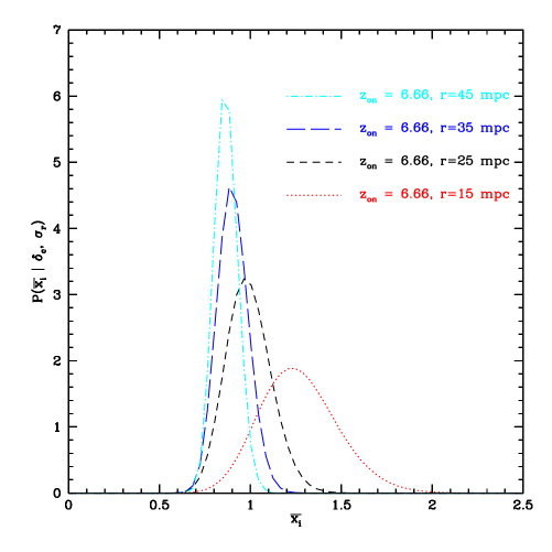
Figure 2.— Probability distribution for the spherically-averaged ionization fraction when the $z=6.42$ quasar turns on in our model for several different smoothing scales. The curves show pdfs for the fraction of the volume that is ionized in regions of different size centered on the quasar host halo. A fraction of $x_{i}\geq 1$ simply indicates that there are enough photons to ionize the entire volume of the region in question.

We can also examine the full probability distribution of the spherically-averaged ionization fraction around quasar host halos, rather than just the mean of this distribution. The results of this calculation are shown in Figure 2 for $M_{\rm halo}=10^{13}M_{\odot}$ and $M_{\rm min}=M_{\rm cool}$ at $z_{\rm on}=6.66$. Note that the curves extend in some cases beyond $x_{i}=1$, which just implies that there are more than enough photons to ionize the entire region in question. On small smoothing scales, there is significant scatter in the ionization from host halo to host halo. Indeed, there is some probability that a region will be less ionized than the cosmic mean, although essentially all host halo regions are more than $60-70\%$ ionized in this model. This scatter is potentially important for quasar proximity zone observations.

In models where rarer sources dominate the ionizing photon budget, we expect the tendency for overdense regions to reionize first to be enhanced. Indeed, since reionization progresses most rapidly in such models, they represent the most plausible scenarios in which the IGM is considerably neutral at quasar turn-on yet highly ionized by $z=6$ (Figure 1). On the other hand, we ignored recombinations in our analysis, and these should lessen the tendency somewhat for overdense regions to ionize first (e.g. Wyithe & Loeb 2006b), although the precise impact of this process will depend on the number of recombinations per hydrogen atom during reionization, which is uncertain.

2.3. Quasar Host Galaxy: Ionizing Photon Budget from Stellar and Quasar Activity

A separate but related question regards the relative contribution of starburst and quasar activity to the cumulative budget of ionizing photons released by the quasar host galaxy alone (see also Yu & Lu 2005, Wyithe & Loeb 2006a). Indeed, the $z\sim 6$ quasar hosts contain $\sim$ solar metallicity gas suggesting substantial levels of prior star formation (e.g. Barth et al. 2003). Our previous arguments imply that neighboring galaxies reionize much of the surrounding IGM before the highest redshift quasar turns on. Here, we focus solely on the budget of ionizing photons produced within the quasar host galaxy itself.

We can estimate the cumulative output of ionizing photons from quasar and stellar sources on the basis of energetic arguments, combined with assumptions regarding the radiative efficiency, the escape fraction of ionizing photons, and the spectral energy distribution of emitted radiation from quasars and stars respectively, along with an assumed relation between black hole and stellar mass. A galaxy with a stellar-mass, $M_{\star}$, produces a cumulative number of ionizing photons (escaping into the IGM) given by $N_{\rm ion,\star}\sim f_{\rm esc,\star}N_{\gamma}M_{\star}/m_{p}$. Here, $N_{\gamma}$ is the number of ionizing photons produced per stellar baryon, $f_{\rm esc,\star}$ is the escape fraction of stellar ionizing photons, and $m_{p}$ is the proton mass. The energy radiated while forming a black hole of mass $m_{\rm BH}$ is $E_{\rm rad}\sim\epsilon_{\rm rad}m_{\rm BH}c^{2}$, for a radiative efficiency of $\epsilon_{\rm rad}$. Assuming that a fraction $f_{\rm ion}$ of this energy comes out in ionizing photons, with a fraction $f_{\rm esc,BH}$ of such photons escaping into the IGM at a mean energy of $\langle h\nu\rangle_{\rm ion}$, the cumulative number of ionizing photons produced by quasar activity is $N_{\rm ion,BH}\sim f_{\rm ion}f_{\rm esc,BH}\epsilon_{\rm rad}c^{2}/\langle h\nu\rangle_{\rm ion}$. We are interested in the ratio of photons produced by quasar and stellar activity. We estimate this ratio assuming that the local Magorrian relation connecting stellar and black hole mass is upheld at high redshift, as supported by the $z\sim 6$ black hole growth simulations of Li et al. (2006). We assume typical values for the other parameters (e.g. Cohn & Chang 2006) arriving at:

$$\frac{N_{\rm ion,\star}}{N_{\rm ion,BH}} \sim\frac{f_{\rm esc,\star}}{f_{\rm esc,BH}}N_{\gamma}\frac{M_{\star}}{M_{\rm BH}}\frac{\langle h\nu\rangle_{\rm ion}/f_{\rm ion}}{\epsilon_{\rm rad}m_{p}c^{2}}$$

$$\sim\frac{0.1}{1}\times 4000\times 2000\times\frac{30eV/0.3}{10^{8}eV}=0.8.$$

For our fiducial parameters, the cumulative numbers of ionizing photons from quasar and stellar activity associated with the quasar host galaxy alone are already comparable, although uncertainties in these parameters may allow this conclusion to change by $\sim$ an order of magnitude. For example, if the quasar turns on before most of the stars and lies off of the local Magorrian relation, the ratio of stellar to quasar photons will be smaller than in the above ratio. This late star formation scenario may be in tension with the presence of $\sim$ solar metallicity gas in the quasar host as mentioned above. We view this simple estimate as a further argument that one needs to consider the ionization from surrounding galaxies, in conjunction with that from the quasar itself, in order to model high redshift quasar proximity zones. On the other hand, note that although quasar and stellar activity associated with the quasar host galaxy cumulatively produce comparable numbers of ionizing photons, the instantaneous photoionization rate from the quasar greatly exceeds that from stars during the lifetime of the quasar (see §4).

3. 3D Radiative Transfer Calculations

In this section, we use 3D radiative transfer calculations to visualize the effects discussed above, and to detail the plausible ionization state of the IGM when the highest redshift quasar turns on. Here we aim to characterize the ionization field produced by high redshift galaxies prior to quasar turn-on, and to quantify its inhomogeneities.

3.1. Simulations

We use the 3D radiative transfer calculations from McQuinn et al. (2006a). These simulations follow the growth of HII regions in a cubic box of co-moving side-length $L_{\rm box}=65.6$ Mpc/$h$. The radiative transfer calculations start from an N-body simulation run with an enhanced version of Gadget-2 (Springel 2005), tracking $1024^{3}$ dark matter particles, and resolving dark matter halos with mass $M\gtrsim 2\times 10^{9}M_{\odot}$. Ionizing sources are placed in simulated dark matter halos, using a simple prescription to connect ionizing luminosity and halo mass (Zahn et al. 2006). Our fiducial ionizing source prescription is identical to that described in Lidz et al. (2006b): halos with mass larger than $M_{\rm min}=2\times 10^{9}M_{\odot}$ host ionizing sources, with an ionizing luminosity proportional to halo mass. The simulated dark matter density field is then interpolated onto a $512^{3}$ Cartesian grid, and we subsequently assume that the gas density closely tracks the simulated dark matter density field (see Zahn et al. 2006 for a discussion). Finally, radiative transfer is treated in a post-processing stage using the code of McQuinn et al. (2006a), a refinement of the Sokasian et al. (2001, 2003, 2004) code, which in turn uses the adaptive ray-tracing scheme of Abel & Wandelt (2002).

How sensitive are the HII bubble sizes at different stages of reionization to the details of our modeling? McQuinn et al. (2006a) demonstrate that the size distribution of HII regions during reionization depends most strongly on the ionized fraction, and is less sensitive to the precise redshift at which a given ionization fraction is reached, and other details of the reionization process. These authors did find, however, larger HII regions at a given ionized fraction if rare, highly biased sources produce most of the ionizing photons. Furthermore, if mini-halos survive pre-heating and are sufficiently abundant during reionization, this reduces the characteristic HII region size (Furlanetto & Oh 2005, McQuinn et al. 2006a). Note that the minimum source mass in our fiducial simulation is $\sim 10M_{\rm cool}$, but even if this is a slight overestimate it should have little impact on the bubble size distribution at fized ionization fraction (McQuinn et al. 2006a). In this paper we adopt the fiducial source prescription mentioned above – we refer the reader to the earlier papers for details regarding the model dependence of our bubble size distributions.

We now characterize the ionization field around plausible quasar host halos. In practice, we examine outputs at several different redshifts and ionization fractions. However, based on the McQuinn et al. (2006a) findings, we expect this to be roughly equivalent to examining the ionization field at fixed redshift, yet varying ionization fraction. Hence, we generally parameterize our partly neutral models by the volume-weighted ionization fraction.

3.2. Ionization Maps

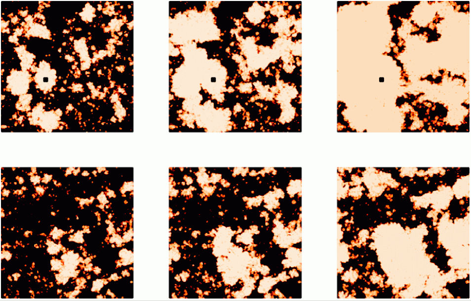
Figure 3.— Ionization fields around a plausible $z\gtrsim 6$ quasar host halo, compared to the ionization in a typical region of the IGM. Top panel: The ionization field in a thin slice ($0.13$ Mpc/$h$ thick, with a side-length of $L_{\rm box}=65.6$ Mpc/$h$) around a halo which may subsequently house a $z\gtrsim 6$ quasar. The slices show different stages of reionization in this overdense environment, when the globally-averaged, volume-weighted ionization fraction is $\langle x_{i}\rangle=0.31,0.48$, and $0.70$ (from left to right). The white regions denote ionized gas, while black regions show neutral gas. The black square indicates the location of the quasar host halo. Bottom panel: For contrast, the ionization field in thin slices through random regions of the IGM at the same global ionization fractions as in the top panel. Comparing the top and bottom panels, it is clear that reionization is accelerated in the overdense regions that will subsequently host the $z\sim 6$ quasars. This results because galaxy formation occurs earlier in overdense regions.

First, we use our radiative transfer simulation simply to visualize the trends suggested by the analytic arguments of the previous section. In Figure 3 we show thin slices ($1$ cell thick = $0.13$ Mpc/$h$) through the simulated ionization field at three different stages during reionization (volume-weighted ionization fractions of $\langle x_{i}\rangle=0.31,0.48$, and $0.70$). In the left-hand side panels we show the ionization field close to a plausible quasar host halo (with $M_{\rm halo}=3\times 10^{12}M_{\odot}$). For contrast, in the right-hand side panels we show the ionization field through random slices of the same simulation outputs.

The figure provides a clear visualization of several points alluded to in the previous section. First, overdense environments are more ionized than typical regions: the eventual quasar host halo is surrounded by a large HII region blown out by galaxies born before the quasar itself turns on. Second, the HII regions are themselves correlated over large scales and so the host halo bubble tends to be surrounded by large neighboring HII regions. These features are seen clearly at each of a few different stages during reionization by contrasting the region containing the quasar host halo in the left panel with the random regions shown in the right panel. The bottom two panels are likely more relevant than the top panels given the arguments of the previous section which suggest $\langle x_{i}\rangle\gtrsim 0.5$ at quasar turn-on. Note also that our limited simulation volume likely impacts our ability to capture large HII bubbles at the end of reionization. In particular, while our general point should be robust to our limited simulation volume, the detailed results may be affected – particularly at $\langle x_{i}\rangle=0.7$ – as one might expect from the large HII regions shown in Figure 3.

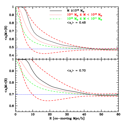
Figure 4.— Spherically-averaged ionization fraction centered on halos of different mass, as a function of radius. The solid black, red dotted, and green dashed lines indicate the average ionization fraction surrounding massive halos from the simulation, while the red dashed band gives the $1-\sigma$ spread across different halos in the middle mass bin ($10^{11}M_{\odot}\leq M<10^{12}M_{\odot}$). The horizontal blue dotted line indicates the ionization fraction averaged over the entire simulation volume. The top panel shows the average ionization around massive halos when $\langle x_{i}\rangle=0.48$, while the bottom panel gives the same at $\langle x_{i}\rangle=0.70$. Reionization happens earlier around the overdense regions that house massive halos in our simulation, and hence the surrounding IGM is more ionized than typical regions.

3.3. Statistical Description of Ionization Fields around Quasar Progenitors

We can quantify the qualitative features of Figure 3 in two useful ways. The first such statistical measure is to compare the average ionization fraction in spheres of different size, with each sphere centered on a massive halo. This calculation is essentially a simulation version of the analytic calculation shown in Figure 2. For comparison, we show the results at each of $\langle x_{i}\rangle=0.48$ (roughly the most neutral case plausible when the $z\gtrsim 6$ quasars turn on, as discussed in the previous section), and $\langle x_{i}\rangle=0.70$ for three different mass bins. For each mass bin, regions surrounding massive halos are on average more ionized than the cosmic mean ionization level. As we discussed previously, this ‘bias’ results because overdense regions contain more halos and hence ionizing sources and reionize earlier than typical regions. This bias is naturally most significant for the largest simulated halos, which are likely hosts for the $z\sim 6$ SDSS quasars. Indeed, Figure 4 demonstrates that the spherically averaged ionization around simulated halos with $M\gtrsim 10^{12}M_{\odot}$ exceeds the cosmic mean ionization out to scales of $R\sim 40$ Mpc/$h$, and $75\%$ of the volume is typically ionized within spherical shells of radii $R\lesssim 10$ Mpc/$h$, and $R\lesssim 25$ Mpc/$h$ at $\langle x_{i}\rangle=0.48$ and $\langle x_{i}\rangle=0.70$ respectively. The true bias is potentially even larger, since the $z\sim 6$ quasars may reside in even rarer, more massive halos than contained in our simulation volume (Haiman & Loeb 2001, Fan et al. 2001, Li et al. 2006). Our most massive simulated halo at this redshift has a dark matter mass of $M_{h}=3\times 10^{12}M_{\odot}$.

Also relevant is the level of halo-to-halo scatter in the spherically averaged ionization fraction. In Figure 4 we show the $1-\sigma$ scatter across halos in the mass bin with $10^{11}M_{\odot}\leq M<10^{12}M_{\odot}$. The scatter is quite significant: for example, there are regions of $R\gtrsim 10$ Mpc/$h$ centered on massive halos that are less ionized than the cosmic mean, even though such regions are on average more ionized than the cosmic mean level. This scatter indicates that variations in the initial ionization field around quasar host halos are substantial, and can potentially lead to significant sightline-to-sightline scatter in the proximity zone size – provided that these observations indeed probe the pre-reionization IGM. The simulation results shown here are also roughly consistent with the analytic calculations of Figures 1 and 2.

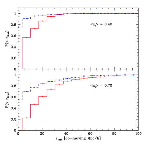
Figure 5.— Cumulative probability distribution for first crossing neutral cells. The top panel shows results for an ionization fraction of $\langle x_{i}\rangle=0.48$, while the bottom panel shows the probability distribution at $\langle x_{i}\rangle=0.70$. In each panel, the red solid histogram gives the first-crossing distance for random sightlines emanating from probable quasar host halos, before the quasar turns on. The blue dashed histogram shows, for contrast, the first crossing distance for sightlines emanating from a random point in the IGM. The first crossing distributions are quite broad, and lines of sight from probable quasar host halos may extend for a length comparable to the purported proximity zone size ($L\sim 40Mpc/h$) before touching any neutral cells, even prior to quasar turn-on.

While the spherically averaged ionization fractions shown above are illustrative, a $1D$ statistic is more relevant for interpreting quasar absorption spectra. As an example, we extend lines of sight from the massive halos in our simulation box and calculate the distance traveled along each line of sight before crossing neutral material. In practice we define a cell to be neutral when the HI photoionization rate averaged over the cell is less than $10^{-5}$ times the cosmic mean photoionization rate. Our general point is, however, insensitive to this somewhat arbitrary definition. The results of this calculation are shown in Figure 5, where we construct the cumulative probability distribution of ‘first neutral crossings’ calculated from 100 lines of sight, cast at random directions from each simulated halo with $M_{\rm halo}>10^{12}M_{\odot}$. We consider the first crossing distribution when the volume-weighted ionization fraction of the IGM is each of $\langle x_{i}\rangle=0.48$ and $\langle x_{i}\rangle=0.70$. The probability distributions shown in the figure are quite broad, and the mean first crossing distance from lines of sight towards quasar host halos is large. Specifically, at $\langle x_{i}\rangle=0.48$, the mean and $95\%$ upper limit for the first crossing distance are $13$ and $28$ Mpc/$h$ respectively, while the corresponding numbers are $24$ and $61$ Mpc/$h$ at $\langle x_{i}\rangle=0.70$. Hence, even in partly neutral scenarios, long skewers towards quasar hosts will traverse entirely through ionized bubbles before the quasars themselves turn on. Indeed if the $z\gtrsim 6$ quasars turn on during the later stages of reionization, a sizable fraction of skewers should pass entirely through ionized bubbles out to length scales even larger than $\sim 40$ Mpc/$h$ – comparable to the purported size of proximity zones inferred from the highest redshift quasar spectra (e.g. Wyithe et al. 2005a). This indicates that the proximity zone sizes deduced from quasar spectra are not primarily determined by the volume-weighted neutral fraction of the IGM, as we discuss subsequently.

In summary, if the $z\gtrsim 6$ quasars truly probe the pre-reionization IGM, the initial ionization field prior to quasar turn on will be inhomogeneous even on quite large scales. Moreover, quasars are biased tracers, residing preferentially in overdense regions, likely ionized before typical regions in the IGM. On spherical average, this bias will be relatively small once one averages over scales of $\gtrsim 30$ Mpc/$h$. Nonetheless, 1D skewers through the IGM may pass entirely through ionized bubbles out to considerably larger scales. This is another example of aliasing, where fluctuations in a random field along skewers of a given length are much larger than those from averaging the same field over spheres of comparable diameter (Kaiser & Peacock 1991). These results contradict the previous wisdom that $z\sim 6$ quasar proximity zones probe sufficiently large scales that ionization inhomogeneities average out, allowing one to model the surrounding IGM with some uniform, yet low level ionization field. In fact, our results suggest that these large scale inhomogeneities significantly complicate the interpretation of $z\sim 6$ quasar proximity zones. In order to understand the precise implications of these initial inhomogeneities, we now consider the subsequent propagation of quasar ionization fronts.

4. Quasar Ionization Fronts and 1D Radiative Transfer

In this section we follow the propagation of quasar ionization fronts using the calculations of the previous section as ‘initial conditions’ and considering, in particular, the difference between the patchy-reionization models discussed above and partly neutral models with some low level uniform ionization, as assumed by most previous modelers.

It is important to keep in mind that our ultimate goal is to construct mock Ly$\alpha$ forest absorption spectra for each scenario and compare with observations. In this sense, our results will be sensitive to the precise values of the residual neutral fraction within the ionized bubbles shown in Figure 3. For example, if residual neutral fractions are at the $\sim 10^{-3}$ level, the Ly$\alpha$ absorption spectra will be very different than if residual neutral fractions are instead only $\sim 10^{-4}$. This is in contrast to simulations of the 21 cm signal during reionization, for which the bubbles of Figure 3 are simply ‘holes’ of effectively zero signal, and one is hence insensitive to the small residual neutral fraction in the interior of the bubbles (apart from occasional dense clumps of more neutral gas which fill only a small fraction of the interior volume). Simulating Ly$\alpha$ absorption spectra in the pre-reionization epoch is therefore more challenging than characterizing the large-scale 21 cm signal. Moreover, our 3D radiative transfer code assumes a sharp ionization front, simply tracking the position of the edge of the ionization front, and assuming ionization equilibrium within the front. Our 3D calculations also ignore helium and assume a uniform temperature within the front. These approximations speed up our 3D calculations substantially, and they are likely very accurate for capturing the size distribution of HII regions during reionization, and the 21 cm signal. However, they may be inadequate for our present purposes: here we want the precise residual neutral fraction and thermal structure within bubble interiors after ionization from quasars. Our usual approximations are especially dubious given that quasars have a hard spectrum of ionizing photons.

In order to do optimize our method, we supplement our 3D analysis from the previous section with more detailed 1D radiative transfer calculations, tracking the subsequent ionization from the quasar. Here our technique is similar to that of Bolton & Haehnelt (2006). This approach is also natural for this application since quasar absorption spectra probe only 1D skewers through the IGM. Our 1D calculations self-consistently solve for the optical depth, the ionization balance, and the temperature of the gas after the quasar turns on. We do not track the hydrodynamic response of gas to the ionization fronts. Of course our 1D approach is also an approximation, but we expect it to be a good one.

4.1. Model Parameters

Before proceeding with our 1D calculations, we briefly discuss several uncertain parameters that go into our subsequent modeling. The first relevant quantity is the size distribution of HII regions at different stages of reionization, as mentioned in the previous section. This depends primarily on the nature of the ionizing sources and the abundance of mini-halos and Lyman-limit systems (Furlanetto & Oh 2005, Furlanetto et al. 2006c, McQuinn et al. 2006a). In the present paper, we consider only the fiducial ionizing source prescription described in the previous section. If mini-halos/Lyman-limit systems are abundant, then the pre-quasar HII regions will be smaller than assumed here, while if rarer sources produce most of the ionizing photons, the HII regions will be larger (see McQuinn et al. 2006a for quantitative details).

4.1.1 Hydrogen Photoionization Rates

Even given the size distribution of HII regions, the precise hydrogen photoionization rate within bubble interiors is somewhat uncertain. It depends on the precise nature of the ionizing sources, the abundance of Lyman-limit systems and the mean free path for ionizing photons in the bubble interiors, and other factors. In principle, one would hope to model all of these quantities self-consistently. In practice, we believe that the precise photoionization rates calculated from our 3D simulations for a given model are less robust than our predictions of the bubble size distribution and 21 cm signal. Owing to this, we will extract only the spatial fluctuations in $\Gamma_{\rm HI}$ ($\Delta_{\Gamma}(\vec{x})=\Gamma_{\rm HI}(\vec{x})/\langle\Gamma_{\rm HI}\rangle$) directly from our 3D simulation, and treat the spatial average as a free parameter. In our fiducial calculations, we somewhat arbitrarily normalize the volume-averaged HI photoionization rate to $\langle\Gamma_{\rm HI}\rangle=10^{-13}s^{-1}$ (we adopt this value for both our $\langle x_{i}\rangle=0.48$ and our $\langle x_{i}\rangle=0.7$ model). This is, however, similar to the values measured directly from our simulation: $\langle\Gamma_{\rm HI}\rangle=9.6\times 10^{-14}s^{-1}$ at $\langle x_{i}\rangle=0.48$, and $\langle\Gamma_{\rm HI}\rangle=2.2\times 10^{-13}s^{-1}$ at $\langle x_{i}\rangle=0.7$. In §5.3 we examine the sensitivity of mock Ly$\alpha$ absorption spectra to this choice.

For clarity, we pause here to point out the significant distinction between the hydrogen photoionization rate in a uniformly ionized medium, and that in a ‘patchy reionization’ model. In a uniformly-ionized IGM, photoionization equilibrium implies a one-to-one relation between the neutral fraction at a given density and the hydrogen photoionization rate. It is easy to see that the volume-averaged hydrogen photoionization rate in our patchy reionization models will be vastly different than that in a uniformly-ionized IGM of the same (low-level) mean ionization fraction.

Let us illustrate this point explicitly by considering two toy models. In the first case, representing patchy reionization, we imagine equal-sized ionized bubbles each with an interior neutral fraction $X_{\rm IN}<<1$, filling a fraction $f$ (with $0<f<1$) of the volume of the IGM, which is otherwise completely neutral. For simplicity, we neglect helium and consider an IGM with a uniform density and thermal state. In the second model, representing ‘uniform ionization’, the neutral fraction is identical at each location within the IGM with $X_{\rm HI}=\langle X_{\rm HI}\rangle=1-f$. In each case, photoionization equilibrium tells us that $\langle\Gamma_{\rm HI}\rangle=\langle\alpha n_{H}\rangle\langle(1-X_{\rm HI})^{2}/X_{\rm HI}\rangle$. Now, in a uniformly-ionized IGM we get $\langle\Gamma_{\rm HI}\rangle_{\rm uniform}=\langle\alpha n_{H}\rangle f^{2}/(1-f)$. In the toy patchy model, we have $(1-X_{\rm HI})^{2}/X_{\rm HI}\sim 1/X_{\rm IN}$ inside each ionized bubble, and $(1-X_{\rm HI})^{2}/X_{\rm HI}\sim 0$ outside of ionized regions. Hence, $\langle\Gamma_{\rm HI}\rangle_{\rm patchy}\sim\langle\alpha n_{H}\rangle f/X_{\rm IN}$. The ratio of the volume-averaged photoionization rates is just $\langle\Gamma_{\rm HI}\rangle_{\rm patchy}/\langle\Gamma_{\rm HI}\rangle_{\rm uniform}\sim(1-f)/(fX_{\rm IN})$. This will typically be a very large number: for example, if $50\%$ of the volume is filled by ionized bubbles ($f\sim 1/2$) each with an interior neutral fraction of $X_{\rm IN}\sim 10^{-4}$, the volume averaged photoionization rate is a factor of $\sim 10^{4}$ times larger in the patchy-reionization model than in the uniform model. Hence the volume-averaged photoionization rates in our models are substantially larger than a reader accustomed to a uniformly-ionized IGM might anticipate. There is also no simple one-to-one relation between volume-averaged photoionization rate and neutral fraction, although the photoionization rate should generally increase as a larger fraction of the IGM is ionized, and each point in the IGM is influenced by more ionizing sources.

In order to give some sense for the model dependence of our adopted photoionization rates, we follow Furlanetto & Oh (2005) and relate the hydrogen photoionization rate to the halo collapse fraction and mean free path to ionizing photons. In this model, the (total) proper ionizing emissivity is given by $\epsilon\sim\zeta\langle n_{H}\rangle df_{\rm coll}/dt$, where $\zeta$ is the ionizing efficiency parameter of Equation (1), $\langle n_{H}\rangle$ is the (average) proper abundance of hydrogen atoms, and $df_{\rm coll}/dt$ is the time derivative of the collapse fraction. Assuming that the mean free path to ionizing photons scales as $\nu^{3/2}$ (Zuo & Phinney 1993, §5.4), we then have:

$$\langle\Gamma_{\rm HI}\rangle \sim\zeta\langle n_{H}\rangle\frac{df_{\rm coll}}{dt}\sigma_{\rm HI}\frac{\alpha}{\alpha+1.5}\lambda_{\rm LL}=10^{-13}s^{-1}$$ (6)

$$\times\left[\frac{\zeta}{11}\right]\left[\frac{|df_{\rm coll}/dz|}{0.03}\right]\left[\frac{1+z}{7.5}\right]^{11/2}\left[\frac{\lambda_{\rm LL}(z)}{2\rm{Mpc}}\right].$$

In this equation, $\sigma_{\rm HI}$ is the hydrogen photoionization absorption cross section at the hydrogen ionization edge, which is numerically $\sigma_{\rm HI}=6.3\times 10^{-18}$ cm². The quantity $\lambda_{\rm LL}$ represents the proper mean free path to ionizing photons at the Lyman limit frequency (see §5.4 for comments on plausible values). The values of $\zeta$ and $df_{\rm coll}/dz$ above are chosen for $M_{\rm min}=10M_{\rm cool}$ and so that $\langle x_{i}\rangle\sim 1$ at $z\sim 6$, assuming the mass function follows the Press-Schechter (1974) form. It is interesting to note that our fiducial hydrogen photoionization rates are a bit higher than the values Fan et al. (2006) infer from their mean absorption measurements on the basis of the Miralda-Escudé et al. (2000) density pdf. Our values are, however, more compatible with constraints from Becker et al. (2006a) derived using a lognormal model for the Ly$\alpha$ opacity. We do caution against over-interpreting this, given the large uncertainties in our modeling. The above expression is only meant to loosely illustrate the model dependence of our adopted photoionization rates.

4.1.2 Quasar Lifetimes and Lightcurves

Next, let us consider the quasar lifetime and ionizing luminosity. In our fiducial model, we adopt $t_{q}=3.6\times 10^{7}$ years for the quasar lifetime. This is our closest time output to a Salpeter time (Salpeter 1964), $t_{s}\sim 4.5\times 10^{7}$ years, assuming a radiative efficiency of $\epsilon_{\rm rad}=0.1$ and Eddington-limited accretion. This timescale is comparable to observational estimates of quasar lifetimes (e.g. Martini 2004) and also roughly to the lifetime derived from numerical simulations of black hole growth (Springel et al. 2005, Hopkins et al. 2005). (In fact, the simulations of black hole growth indicate that the quasar lifetime depends on luminosity, but the Salpeter time is a reasonable measure of the timescale during which most of the black hole mass is accumulated; see e.g., Hopkins et al. 2006; Hopkins, Richards & Hernquist 2007.) However, the quasar lifetime is still uncertain observationally by $\sim 2$ orders of magnitude (Martini 2004). Consequently, we also consider $t_{q}\sim t_{s}/10$ in which case it is generally easier to locate the edge of a quasar proximity zone observationally (§5). Note, however, that decreasing the quasar lifetime increases the challenge of growing supermassive black holes by $z\sim 6$ (Haiman & Loeb 2001, Li et al. 2006). In our fiducial model, we adopt an ionizing luminosity of $\dot{N}=1.8\times 10^{57}$ photons per second, corresponding roughly to the mean ionizing luminosity of the Fan et al. (2006) $z\sim 6$ quasar sample, provided their spectra match the Telfer et al. (2002) quasar composite spectrum. For reference, the brightest quasar in the Fan et al. (2006) sample is roughly $\sim 2$ times brighter than this, while the faintest quasar is $\sim 3$ times fainter. For simplicity we assume here that quasars radiate steadily at this luminosity for their entire lifetime (but see § 6).

Finally, the level of small scale structure in the IGM is highly uncertain and can affect our results. We examine the impact of small scale structure on our mock absorption spectra in the next section: here we present results without including any ‘subgrid-clumping’.

4.2. Results from Our 1D Calculations

As input for our 1D radiative transfer calculations we extract $20$ random lines of sight towards each of the five most massive halos in our simulation box at $z\sim 6.6$. These halos have masses in the range $1.4\times 10^{12}M_{\odot}<M_{h}<3.1\times 10^{12}M_{\odot}$. We simulate quasars at $z_{q}=6.42$, corresponding to the highest redshift source in the Fan et al. (2006) sample. We project each sightline at a random angle with respect to our simulation box, interpolating the density and peculiar velocity fields (needed to construct mock absorption spectra) from our N-body simulation. Each sightline wraps around our periodic simulation box and extends for $130$ co-moving Mpc/$h$. Our 3D calculations are not ‘in the light-cone’ and so we ignore redshift evolution in the ionization state of the gas across each sightline.

For convenience in performing our radiative transfer calculation, and generating mock quasar spectra, this interpolation is performed using a fine grid with $1500$ cells. Moreover, we interpolate the HI photoionization rate from our 3D calculations onto each line of sight. This specifies a (fluctuating) galactic ionizing background which is incorporated as we calculate the subsequent ionization from our quasar source. We approximate the galactic background ionization as fixed over the quasar lifetime, $t_{q}\sim t_{s}\sim 4\times 10^{7}$ yrs. From the simulated HI photoionization rate, we specify a fluctuating background HeI photoionization rate (our 3D calculations ignore helium and hence do not track HeI photoionization), assuming a galactic ionizing spectrum that follows a $\nu^{-2}$ power-law near the HI/HeI photoionization edges. We further assume that our galactic sources do not contribute any photons capable of doubly ionizing helium. Finally, we assume that cells ionized by galaxies in our 3D calculations are uniformly heated to $T=10^{4}K$ (gas temperature is not tracked in our 3D calculations). Neutral cells are assumed to be initially at the CMB temperature, but our results would be unchanged for any other small temperature.

Our 1D radiative transfer calculations follow the C2-ray scheme of Mellema et al. (2006a), generalized to include helium and to track the thermal state of the gas in the IGM. We refer the reader to the Mellema et al. (2006a) paper for a description, and we will present details of our implementation elsewhere, but a few pertinent comments are as follows. We make use of the fact that, along the line of sight in the frame of the observer, the quasar front obeys the non-relativistic I-front equation, and so there is no need to impose finite speed of light constraints (see Cen & Haiman 2000, Bolton & Haehnelt 2006 and references therein). In order to rapidly compute photoionization and photoheating rates, we adopt approximate forms for the frequency dependence of the opacity between the HeI and HeII edges and above the HeII photoionization edge. This allows us to compute photoionization and photoheating rates from lookup tables after specifying just the optical depth in each of three frequency bins (see Shapiro et al. 2004 for a similar scheme). We use the thermal and chemical rates from Hui & Gnedin (1997). Our code has been tested against the usual analytic solutions for I-front propagation in a homogeneous IGM.

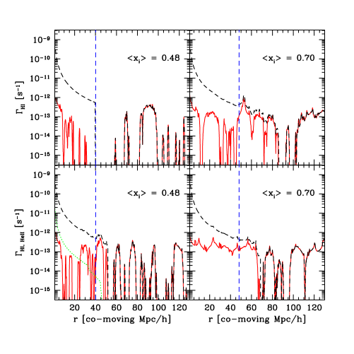
Figure 6.— Photoionization rate of HI and HeII from our 1D radiative transfer calculations as a function of separation ($r$) from the quasar. The left panels show the photoionization rates along two random lines of sight through our simulation box, for a case in which the quasar turns on when $48\%$ of the simulation volume is ionized. The red solid line shows the initial photoionization rate contributed by galactic sources, before the quasar itself turns on. The black dashed line shows the photoionization rate after the quasar has shined for $t_{q}\sim t_{s}$, reflecting the combined radiation field of the quasar and background galaxies. The blue dashed line shows the expected location of a quasar HII front in an IGM with a uniform ionization level of $48\%$. The top line of sight intersects many neutral patches, and the quasar front halts around the expected position in a uniform medium. In the bottom panel, the front passes through longer stretches of ionized gas and extends further. The green dotted line in the bottom panel shows the relatively broad quasar HeII front (for visual clarity we omit the HeII curve in the other panels). The right panels are identical for sightlines in which $70\%$ of the volume is ionized when the quasar turns on. Since quasars are born into large HII regions, the typical sightline extends further than expected in a uniform medium.

We show results from our 1D calculations in Figure 6 for our fiducial model with initial (pre-quasar) volume-averaged ionization fractions of $\langle x_{i}\rangle=0.48$ and $0.70$. Consider first the combined HI photoionization rate from galaxies and quasars (indicated by the black dashed lines in Figure 6): at small separations, the quasar strongly dominates the photoionization rate and there is a relatively smooth $\sim 1/r^{2}$ fall-off, while the HI photoionization rate fluctuates significantly at larger distances from the quasar. The extent of the $\sim 1/r^{2}$ run indicates the maximum distance the quasar front reaches over the quasar lifetime along a given sightline: the front halts at some distance upon crossing sufficient quantities of neutral gas, and subsequently there is only photoionization from background galaxies. The photoionization from background galaxies itself fluctuates owing to the presence of neutral stretches of gas, since there is a distribution of bubble sizes at each stage of reionization and the photoionization rate is typically more intense in larger ionized bubbles, and because the photoionization rate fluctuates from place to place within ionized bubbles.

The red solid lines in Figure 6 indicate the initial ionization provided by galaxies before the quasar itself turns on. From the example sightlines, it can be seen that quasar ionization fronts extend further along sightlines with larger levels of ‘pre-ionization’ from background galaxies. For example, the quasar front traverses more neutral material, and extends less far, in the top-left panel than in the bottom left panel, even though both adopt the same quasar lifetime and volume-weighted ionization fraction. Another interesting feature of Figure 6 is that the opacity to ionizing photons at the Lyman-limit frequency from residual neutral material amounts to $\tau\sim 1$ at $r\sim 50$ co-moving Mpc/$h$. Hence, there is some fall-off in excess of $\sim 1/r^{2}$ for lines of sight in which the front extends to large distance, although this is slightly disguised in our figure by upward fluctuations in the galactic photoionization rate. In §5.4 we argue that our simulations may underestimate this residual opacity.

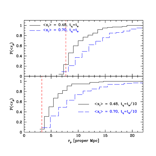
Figure 7.— Cumulative probability distribution of quasar ionization front extents for partly neutral models. Top panel: The cumulative probability distribution of quasar ionization front extents in models with initial volume-weighted ionization fractions of $\langle x_{i}\rangle=0.48$ and $\langle x_{i}\rangle=0.7$. Here we assume a quasar luminosity of $\dot{N}=1.8\times 10^{57}s^{-1}$ and a quasar lifetime of $t_{q}\sim t_{s}$. The red dashed line indicates the expected quasar front position in a uniform IGM with $\langle x_{i}\rangle=0.48$ and $t_{q}\sim t_{s}$. Bottom panel: The same for a quasar lifetime of $t_{q}\sim t_{s}/10$. In each case, the histograms are quite broad owing to the presence of large ionized bubbles created by galaxies before quasar turn-on. The fronts generally extend further than in a homogeneous IGM of the same ionization fraction, since the quasars tend to be born into large HII regions. Occasionally, fronts passing through mostly neutral gas extend slightly less far than in the uniform case owing partly to overdense gas and helium absorption. The scalings for quasar front extent expected in a uniform IGM, $r_{p}\propto t_{q}^{1/3}/<x_{\rm HI}>^{1/3}$, are inaccurate owing to the presence of large galaxy-created HII regions.

The example sightlines of Figure 6 illustrate a diversity of quasar front positions at a given $\langle x_{i}\rangle$, with a strong dependence on the initial galaxy-generated ionization along each sightline, but we require a statistical measure to characterize this quantitatively. In Figure 7, we show the cumulative pdf of ionization front extent, averaged over our ensemble of $100$ sightlines for two partly neutral models and two assumed quasar lifetimes. Here, and in what follows, we show results in units of proper Mpc to match the convention of previous proximity-zone modelers. The vertical dashed lines in each panel illustrate the expected front position in a uniform IGM with $\langle x_{i}\rangle=0.48$. In each case, we see the bias discussed in the previous section: since quasars are born into large HII regions, the fronts extend further on average compared to an IGM that is uniformly ionized (with an ionization fraction equal to the volume-averaged ionization fraction in the patchy reionization case). On the other hand, there are also occasional sightlines that reach less far than expected in a uniform IGM. These sightlines traverse longer neutral stretches than the typical sightline. The presence of overdense gas, and absorption by helium, also act to reduce the front extent compared to the expectation for a uniform IGM. For the majority of sightlines, however, the fronts travel further than expected in a uniform IGM. The average front extends $\sim 25\%$ ($\sim 30\%$) further in our patchy reionized model at $\langle x_{i}\rangle=0.48$ ($\langle x_{i}\rangle=0.70$) – assuming $t_{q}\sim t_{s}$ – than in a uniform IGM.

Moreover, the sightline to sightline scatter in quasar front position is quite large. For example, it takes until $r_{p}\sim 12.9$ ($18.1$) proper Mpc to get to the $84\%$ ($97.5\%$) upper limit on quasar front extent when $\langle x_{i}\rangle=0.48$ and $t_{s}\sim t_{q}$. Clearly quasar ionization fronts can extend much further than in a uniform IGM, where one expects $r_{p}\sim 7.7$ Mpc for $\langle x_{i}\rangle=0.48$, $t_{s}\sim t_{q}$. The bias and scatter are still stronger when the quasar lifetime is shorter, as illustrated in the bottom panel of Figure 7. This occurs because when the quasar lifetime is short the quasar has less time to ionize the surrounding gas and the front extent along an individual sightline is hence even more sensitive to its initial pre-quasar ionization state. The histograms also illustrate that the scalings expected in a uniform IGM, $r_{p}\propto t_{q}^{1/3}/\langle x_{\rm HI}\rangle^{1/3}$, are inaccurate: the extent of the quasar ionization fronts is sensitive to the presence of galaxy-generated ionized pathways. This means that one needs a significant data sample to infer the ionized fraction statistically, as well as a model to connect the probability distribution of proximity zone sizes with the volume-weighted ionization fraction.

It is also interesting to compare the ionization front extents in these models with the ‘proximity’ scale. This scale is relevant for models in which the entire volume of the IGM is ionized and indicates where the photoionization rate from the quasar drops to that of the background radiation field. Ignoring residual opacity along the line of sight (this may overestimate the proximity scale – see §5.4 for comments), this distance is $r_{\rm prox}\sim 18$ proper Mpc $\times$ $\left(\dot{N}/1.8\times 10^{57}s^{-1}\right)^{1/2}\left(\Gamma_{\rm bcknd}/10^{-13}s^{-1}\right)^{-1/2}$. Notice that this scale is comparable to the extent of quasar ionization fronts along many of the sightlines in our partly neutral models, suggesting that it may be difficult to distinguish models on the basis of their Ly-$\alpha$ forest proximity zones. Another way to say this is as follows: for our fiducial parameters, even in partly neutral models there is generally little contrast between the photoionization rate at the edge of the quasar ionization front and that provided by the background galaxies beyond the front (see Figure 6). As we will see in the next section, this makes it challenging to locate the ‘edge’ of the quasar front on the basis of Ly-$\alpha$ absorption spectra. The contrast between the photoionization rate at the front edge and from the background galaxies will be larger than in our fiducial model if $\langle\Gamma_{\rm HI}\rangle$ is smaller than we assume (background galaxies are less intense), or if the quasar radiation field is more intense at the front edge. The quasar will be more intense at the front edge if the quasar lifetime is shorter (although even for a short lifetime quasar fronts will extend to large distances along some sightlines, Figure 7), and more luminous. In practice, however, the brightest quasars in the Fan et al. (2006) sample are only a factor of $\sim 2$ brighter than in our fiducial calculation.

Before constructing mock quasar spectra from our 1D calculations, we briefly discuss helium photoionization rates and the thermal state of the IGM (see also Bolton & Haehnelt 2006). The galaxies that reionize the IGM in our simulations have a soft spectrum and so they mostly singly ionize helium, but do not doubly ionize it. Hence, before the quasar turns on in our calculations, helium is mostly singly ionized and is doubly ionized only by the quasar itself. Because of this, the HeIII front lags behind the HII and HeII fronts. The HeIII front is, however, rather broad owing to the long mean free paths for HeII ionizing photons. Both of these features are illustrated by the green dotted line in the bottom left-hand panel of Figure 6. The HeII front (not shown in the figure for visual clarity), on the other hand, closely tracks the HII front in our calculation. In principle, the position of the quasar HeIII front provides interesting information regarding the ionization state of helium and the quasar lifetime: we can be fairly confident that HeIII, unlike HII, comes from photoionization by the quasar itself. However, HeII Ly$\alpha$ forest observations must be done in the ultraviolet band and are hence challenging (e.g. Shull 2004). Finally, initially neutral regions are raised to temperatures of $30-40,000$ K by the photoheating of HI and HeII (see Abel & Haehnelt 1999, Bolton & Haehnelt 2006). This quasar-heated gas recombines less rapidly, and is more thermally-broadened than the cooler galaxy-ionized gas (which we assume to be initially uniformly heated to $10,000$ K.)

5. Mock Quasar Spectra

At this point, the reader may be curious about two aspects of our line of reasoning. The first point is that, starting with Wyithe & Loeb (2004), several authors have pointed out that the observed $z\gtrsim 6$ proximity zones are small and used this fact to argue for a partly neutral IGM. In the previous sections, we argued that quasar ionization fronts may extend further than assumed by these authors in a partly neutral IGM. One might imagine that this strengthens the case for a partly neutral IGM, or even places our results in conflict with observations. Second, at least some of the sightlines in Figure 6 have sharp ionization fronts and one might assume that it would be relatively easy to detect these sharp features in quasar absorption spectra.

In this section we will address both of these points. First, we illustrate that in our fiducial model, the quasar is dim enough at the ionization front edge that the average transmission through the forest is already very low (§5.1). Generally this means that previous measurements of quasar ionization front extents are underestimates, as pointed out previously by Bolton & Haehnelt (2006) and Maselli et al. (2006). Mesinger & Haiman (2004) also comment on the difficulty of recovering quasar front positions from Ly$\alpha$ forest spectra. On the other hand, they argue that the Ly$\beta$ region can be used in conjunction with the Ly$\alpha$ forest to aid in recovering the position of ionization fronts, although here one needs to contend with the foreground Ly$\alpha$ forest. Here, we describe and test (on mock spectra) an improved algorithm for determining the extent of quasar ionization fronts from Ly$\alpha$ forest spectra (§5.2). We then emphasize the strong dependence of our results on the (highly uncertain) level of small-scale structure in the IGM, and other unknowns (§5.3-§5.4).

5.1. Average Transmission in the Quasar Proximity Zone

We construct mock quasar spectra from the neutral hydrogen density, temperature, and peculiar velocity fields generated from our cosmological simulation, and 1D radiative transfer calculations, in the usual manner (see e.g. Hernquist et al. 1996, Hui et al. 1997). Note that we calculate the optical depth by convolving with the full line profile, including the effects of both thermal broadening and the natural line width, since damping-wing absorption can be significant in our partly neutral scenarios (Miralda-Escudé 1998). Since the damping wings are quite broad, we extend our sightlines slightly (ignoring redshift evolution in the ionization state) in order to accurately calculate the optical depth near the edge of each sightline.

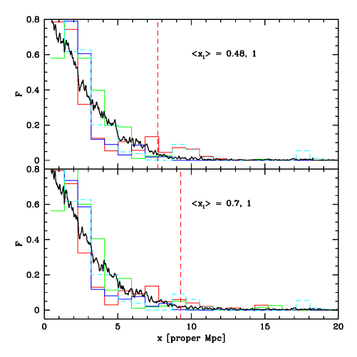
Figure 8.— Mock quasar spectra drawn from each of two partly neutral models and a completely ionized IGM. Bottom panel: The black solid line shows the transmitted flux as a function of distance from the quasar, averaged over a large ensemble of quasar spectra for a patchy-reionization model with $\langle x_{i}\rangle=0.7$. The red, green, and blue histograms show the transmission along several example sightlines from the patchy model, smoothed as in Fan et al. (2006). The cyan dashed histogram shows an example sightline from a completely ionized IGM ($\langle x_{i}\rangle=1$) with the same mean hydrogen photoionization rate as our patchy models. The red dashed line shows the expected ionization front extent in a uniform model with $\langle x_{i}\rangle=0.7$. In all cases, there is transmitted flux beyond this scale, although in §5.3 we show that this depends on the amount of small-scale structure in the IGM. This transmission occurs because quasar fronts tend to extend further in the patchy case than in the uniform, low-level ionization model, and because galaxy-created HII regions beyond the extent of the quasar front can transmit flux. It is hard to distinguish between the highly-ionized and partly neutral models. Top panel: Identical to the bottom panel for a model with $\langle x_{i}\rangle=0.48$.

First, let us consider the average transmission profile around several $z_{q}=6.42$ quasars hosts drawn from our simulation. Specifically, we calculate the transmission using the 1D radiative transfer calculations of the previous section along each of $100$ lines of sight, which were assembled from $20$ random lines of sight towards each of the five most massive halos in our simulation box. Clearly this is for illustrative purposes only, as present data samples consist of only 3–4 quasars with $z\gtrsim 6.2$ (Fan et al. 2006).

To begin with, we consider our patchy reionization model with $\langle x_{i}\rangle=0.7$, and restrict our analysis to the blue side of the quasar Ly$\alpha$ emission line. The $100$-sightline averaged transmission profile for this model is indicated by the solid black line in the top panel of Figure 8. The sightline averaged transmission falls rapidly with increasing distance from the quasar, a direct reflection of the decreasing quasar ionizing flux, which falls off as $\Gamma_{\rm HI,qso}\propto 1/r^{2}$. Indeed, at $\sim 6$ Mpc proper from the quasar the average transmission is only at the $10\%$ level. At still larger separations from the quasar there is only a small residual flux, on average. The transmission at large separations results partly from sightlines that intersect galaxy-created HII regions beyond the extent of the quasar HII front, and partly from sightlines where the quasar HII front itself reaches large distances by passing through several galaxy-generated HII regions. The transmission extends significantly further than quasar fronts do in a uniform IGM of the same ionization fraction, as illustrated by the vertical red dashed line in the figure (see §5.3 for caveats). These features just illustrate the impact of pre-quasar HII regions and the extended and fluctuating photoionizing flux of Figure 6 on the transmission in the Ly$\alpha$ forest.

The top panel of Figure 8 is very similar to the bottom one, except that in this panel the mock spectra are drawn from a model where reionization is less advanced when the quasar turns on ($\langle x_{i}\rangle=0.48$). Comparing the solid line in the two panels, one sees only very subtle differences in the average transmission between the two models.

Note that in our fiducial model, we do typically get some transmission through the Ly$\alpha$ forest beyond the quasar range of influence even when the IGM is $50\%$ neutral (Furlanetto et al. 2004b). This transmission may be overestimated if the IGM is more clumpy than in our model, as we argue subsequently, or if we overestimate the galactic photoionizing background. In order to get transmission through the IGM when it is half neutral, there must also be sufficiently long stretches of ionized gas so that the damping wings from neutral gas on each side of an ionized stretch do not overlap (Miralda-Escudé 1998). If we approximate the IGM as homogeneous on each side of an ionized stretch, with neutral fraction $X_{\rm HI}$, the damping wing opacity (including both redward and blueward of the ionized stretch) amounts to $\tau_{\rm dw}=1$ at the center of the ionized region of size $L\sim 4X_{\rm HI}\sigma_{\alpha}R_{\alpha}n_{\rm H}(z)(c/H(z))^{2}/\pi$ (Miralda-Escudé 1998). Here, $\sigma_{\alpha}$ is the Ly$\alpha$ cross-section, $R_{\alpha}=2.02\times 10^{-8}$ is related to the natural line width, and the other symbols have their usual meanings. When the IGM is $50\%$ neutral, this estimate – which should be an overestimate close to the quasar – requires a stretch of $L\sim 1.8$ proper Mpc. Paths of this length are not rare in our calculations when the IGM is $50\%$ neutral. Hence, resonant absorption may be more of an obstacle for transmission in the partly neutral IGM, than damping wing absorption (Furlanetto et al. 2004b).

Let us now consider transmission spectra on a sightline-by-sightline basis. This is more observationally relevant than the 100 sightline-averaged curve described above, given the limited observational samples available presently. We follow Fan et al. (2006) and top-hat filter our mock spectra at $20\mbox{ \AA}$ resolution, even though their spectra have intrinsically higher resolution. This extra smoothing is performed because as emphasized by Fan et al. (2006), the proximity scale, defined as the first time the transmission crosses some threshold value, is naturally sensitive to the smoothing scale of the observations. Example lines of sight are shown by the solid, colored histograms in Figure 8. For comparison, we also show a sample line of sight (cyan dashed histogram) drawn from a model in which the entire volume of the IGM is ionized. One can immediately see that it is difficult to distinguish between different models for the volume-ionized fraction on the basis of a few absorption spectra alone. The main obstacle is that the transmission is generally very low close to the edge of an ionization front in our models. Comparing with the highest redshift bin in Figure 14 of Fan et al. (2006) it seems, however, that each of our models overproduces the transmission at large distances in comparison to the observations. We return to this shortly in §5.3.

First, in order to further examine our ability to discriminate between models, we construct histograms of first-threshold crossing distances from our smoothed spectra. This has been used by Fan et al. (2006) and others as a diagnostic for ionization-front position. Here we simply record the closest distance to the quasar at which the smoothed-transmission falls below a given threshold, $F_{\rm thresh}$. Using $F_{\rm thresh}=0.1$ as in Fan et al. (2006), we find little difference between models. This is because the IGM is opaque enough at these redshifts that the transmission generally falls below this threshold even within the quasar ionization front, making this measure a poor tracer of ionization front extent. Using a smaller threshold is an improvement, but it is still very difficult to distinguish between models since even the smoothed spectrum frequently falls below the threshold before reaching the front edge. If one chooses a still smaller threshold, then one picks up transmission from background galaxies and misidentifies the front position. Smoothing each spectrum with a $20\mbox{ \AA}$ filter also partly washes out distinctions between models, since the transmission spikes are generally very narrow.

5.2. Improved Algorithm for Determining Quasar-Front Extents

Can we devise a better algorithm to locate the extent of quasar ionization fronts and distinguish between different models? Our basic task is to identify a scheme for locating an ‘edge’ in a quasar absorption spectrum: shortward of the edge, the quasar contributes to the ionizing flux, while longward of the edge only background galaxies contribute. We propose a simple variant of the Fan et al. (2006) first threshold-crossing scheme, based on locating the furthest distance from a quasar, beyond which the (un-smoothed) transmission crosses a given threshold. In locating the ‘last-crossing’ distance, we consider only pixels within $20$ proper Mpc of the quasar. We find that this ‘last-crossing’ scheme is a better diagnostic of quasar front position. It is also advantageous to use the full un-smoothed spectrum to preserve as much information as possible, although some smoothing will be necessary for sufficiently noisy data.

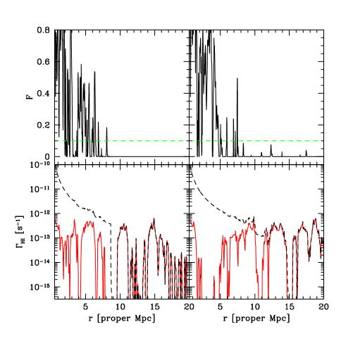
Figure 9.— Illustrative examples of our front-locating algorithm. Here we show an example sightline where our method performs well, and an example where it performs poorly. Each sightline is drawn from our model with $\langle x_{i}\rangle=0.48$. Left-hand panels: Well-recovered front position example. The ionization field (bottom panel), and (un-smoothed) transmission through the Ly$\alpha$ forest (top panel) for a sightline where the edge of the quasar ionization front is recovered relatively accurately. As in Figure 6 the red solid line shows the pre-quasar photoionizing field, while the black dashed line shows the combined quasar and galaxy field. The green dashed line in the top panel indicates an example flux threshold used in recovering the front position. The last place where the transmission crosses the flux threshold is close to the true front position, which corresponds to where the photoionization rate first drops off in the bottom panel (near $\sim 8-9$ proper Mpc). Along this sightline, in spite of the significant galactic photoionizing background, there is no gas that is sufficiently underdense to transmit flux at greater separations from the quasar. Right-hand panels: Poor-recovery example. In this case, the quasar front extends to a considerably larger distance ($r\sim 15$ proper Mpc). The IGM, however, is opaque enough to prevent transmission in excess of the flux threshold beyond $r\sim 8$ proper Mpc. Consequently, along this sightline the true front position is underestimated by nearly a factor of $\sim 2$.

The basic idea of our last-crossing threshold scheme is illustrated by the example sightlines shown in Figure 9. A clean case is shown by the sightline in the left-hand panels, drawn from our fiducial model with $\langle x_{i}\rangle=0.48$. Here, the transmission fluctuates and is reasonably substantial before declining beyond $r\sim 8-9$ proper Mpc. In this case, the last place along the line of sight where the transmission crosses a threshold of $F_{\rm thresh}=0.1$ is a reasonable indicator of quasar ionization front extent, as can be seen in the figure. Along this sightline, it is a slight underestimate (by $\sim 10\%$), owing both to damping wing absorption and since one requires a sufficiently underdense region to allow transmission through the forest. (Note that peculiar velocities also impact the mapping between observed and actual position.) Note that there is also a substantial galactic component to the ionizing flux at larger distances along this sightline. In this case, the surrounding gas is, however, too dense to transmit flux through the Ly$\alpha$ forest.

Along other sightlines, it can be quite difficult to locate the position of the quasar ionization front, and even our improved algorithm can lead to inaccurate results. This is illustrated by the example sightline in the right-hand panels of Figure 9. Along this line of sight, the quasar ionization front extends to a larger distance ($r\sim 15$ proper Mpc), but fails to produce a transmission spike – i.e., transmission exceeding our flux threshold – beyond $r\sim 7-8$ proper Mpc. This is again the difficulty mentioned in the previous sub-section: the transmission at the quasar ionization front edge is generally low, and there is no guarantee of surrounding gas that is underdense enough to transmit any flux. If we lower the flux threshold slightly, our algorithm will pick up the more distant quasar-created transmission spike. However, if we lower the threshold too much, our algorithm will begin to identify the still more distant galaxy-generated spikes.

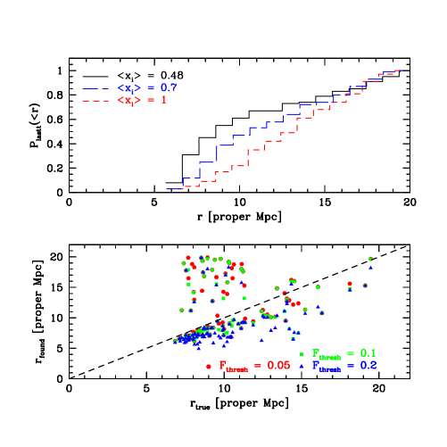
Figure 10.— Test of quasar front position recovery, and power to distinguish between models. Bottom panel: Scatter plot comparing the true quasar front position (x-axis) along a sightline, with the front position recovered using our last-crossing algorithm (y-axis). We show the recovered front positions for each of three flux thresholds. The dashed line indicates perfect recovery: points underneath the line indicate sightlines where our algorithm underestimates the true front position, while points above the line indicate overestimates. Top panel: The cumulative pdf of last-crossing positions (with $F_{\rm thresh}=0.1$) for $100$ sightlines drawn from models with each of $\langle x_{i}\rangle=0.48,0.70$ and $1$ and all other parameters fixed at their fiducial values. This illustrates that even if the error on the recovered front position along an individual sightline is large, we can still hope to distinguish between models given a sufficiently large sample of sightlines. However, the details of this panel are subject to several model uncertainties, particularly the level of small scale structure in the IGM (see §5.3).

In order to characterize the accuracy of our algorithm more quantitatively, we locate the last threshold crossing position for each of $100$ sightlines drawn from our fiducial model at $\langle x_{i}\rangle=0.48$ and compare this with the true quasar front position. The results of this test are shown in the bottom panel of Figure 10. Concentrating on the locus of points near $r\lesssim 8$ proper Mpc, we see that our front recovery algorithm works reasonably well for small quasar front extents along many sightlines. In this case, the true front position is underestimated: this owes to damping wing absorption, and since one needs to pass through an underdense region to transmit any flux. The recovered front position hence, loosely speaking, indicates the last underdense region within the quasar front. The error in the recovered front position can, however, be large as one can see from the many points lying above the dashed line in the figure that indicates perfect front recovery. These points correspond to sightlines where the galactic ionizing background beyond the quasar front gives rise to transmission through the Ly$\alpha$ forest. Along these sightlines, the front-locating algorithm is fooled into thinking that galaxy-created transmission spikes are associated with flux from the quasar, resulting in an overestimate of quasar front position. This source of error is reduced by increasing the flux threshold – and hence reducing the occurrence of ‘false positives’ – but increasing the flux threshold in turn causes one to further underestimate the short-length quasar front positions. Note also that quasar ionization fronts really do extend to large distances along some sightlines, so it is not viable to simply throw sightlines with large front extents out of the analysis. Doing so could easily bias our constraints. Quantitatively, the true front position is recovered most accurately on average for $F_{\rm thresh}=0.05,0.1$, in which case the true front position is identified to within $\pm 20\%$ along $\sim 40\%$ of sightlines for this model. There are however significant outliers as one can see clearly from the figure.

Even though the error in front positions from individual sightlines may be substantial, one can still hope to distinguish between different models statistically, albeit in a model-dependent manner. This is illustrated by the top panel of Figure 10. Here we show the cumulative pdf of recovered front positions for $F_{\rm thresh}=0.1$ at $\langle x_{i}\rangle=0.48,0.70$, and $1$, with our other model parameters fixed at their fiducial values. In this example, we take the idealized case of $100$ quasar spectra with perfect signal-to-noise, resolution and identical quasar luminosity and lifetime. One can clearly see the tendency towards larger last threshold crossing distances as a greater fraction of the volume is ionized, as expected. In the context of this simplified calculation where, for example, all of our quasars have identical lifetimes and luminosities, we expect $\sim 10$ $(30)$ spectra are needed to rule out a completely ionized model at $\sim 1-\sigma$ $(2-\sigma)$ if the real universe has $\langle x_{i}\rangle=0.48$.

As we emphasize in the next subsection, there are important model uncertainties that could impact these predictions. Specifically, the precise mapping between hydrogen photoionization rate and transmission is sensitive to the level of small scale structure in the IGM. If there is less transmission at a given hydrogen photoionization rate than in our model (as may be indicated by the data), then the distance beyond which it becomes hard to locate the true front position ($r\sim 8-9$ proper Mpc in Figure 10) will shrink, and make it harder to distinguish models. On the other hand – in comparison with our fiducial case – increasing the quasar luminosity while decreasing the quasar lifetime, and/or decreasing the intensity of the photoionizing background should make it easier to locate ionization front edges. Finally, following Mesinger & Haiman (2004), applying our algorithm to the Ly$\beta$ forest may be helpful, although here one needs to deal with the foreground Ly$\alpha$ forest. Furthermore, while our last-crossing algorithm is easy to implement, it is not ‘optimal’ in any sense. One might be able to improve on it by, for example, recording the length of dark gaps after last threshold crossing along each sightline. Moreover, if one can indirectly extract the signature of damping wing absorption from the data (Mesinger & Haiman 2004, 2006) this would be a smoking gun for a partly neutral IGM, although uncertainties in the clumpiness of the IGM may complicate this effort (§5.3).

5.3. Sensitivity to Model Details

At this point, we need to emphasize that the ‘mapping’ between photoionization rate and transmitted flux is model dependent, and may not be well captured by our moderate resolution N-body simulations. Specifically, our transmission profiles depend on the clumpiness of the IGM and the mean photoionization rate within galaxy-generated HII regions beyond the quasar range of influence.

We begin by considering the clumpiness in the IGM. After reionization, the relevant scale is the filtering scale (Gnedin & Hui 1998), the distance over which baryonic fluctuations are smoothed owing to finite gas pressure. According to Gnedin & Hui (1998), the filtering scale can easily be a factor of $\sim 10$ smaller than the linear Jeans scale close to reionization, since the gas takes some time to respond to prior photoheating. In our calculations, we assume that the baryons directly trace the dark matter, but density fluctuations are smoothed out by the finite resolution of our simulation. The Nyquist frequency of our simulation grid is $k_{\rm Nyq}\sim 25h$ Mpc^-1. For comparison, if the gas in the IGM is isothermal with a temperature of $\sim 10^{4}K$ at $z=6.5$, then the linear Jeans wavenumber is $k_{J}\sim 15.7h$ Mpc^-1. Given that the filtering wavenumber $k_{F}$ should be at least several times – and potentially more than an order of magnitude – larger than the Jeans wavenumber (Gnedin & Hui 1998), we likely underestimate the small scale structure in the gas density field. This is a consequence of our finite simulation resolution ($k_{\rm Nyq}\sim 25h$ Mpc^-1) and hence, even though we assume that the baryonic density field directly traces that of the dark matter, we may underestimate the clumpiness in the baryon distribution.

This could impact the results shown thus far in two ways. First, we underestimate the number of recombinations during reionization and, consequently, we underestimate the residual neutral fraction within previously ionized cells. Moreover, quasar ionization fronts should extend slightly less far than they do in our calculations (see the next sub-section, §5.4, for related discussions). Second, transmission in the high redshift Ly-$\alpha$ forest is very sensitive to the abundance of rare voids in the IGM (e.g. Oh & Furlanetto 2005, Becker et al. 2006a). Our low simulation resolution artificially suppresses the number of low-density excursions in the gas density field.

In order to explore the impact of the first deficiency in our modeling, we now incorporate a simple model for sub-grid clumping into our calculations. We first estimate plausible levels for the clumpiness in the baryon distribution close to reionization. (For recent related calculations see Kohler et al. 2005, Mellema et al. 2006b, McQuinn et al. 2006a, Trac & Cen 2006; our present work is similar to that of McQuinn et al. 2006a.) We estimate a volume-averaged clumping factor for the baryon distribution by taking $C_{V}=1+\langle\delta_{b}^{2}\rangle$, with $\langle\delta_{b}^{2}\rangle\sim\int d^{3}k/(2\pi^{3})\ \rm{exp}(-2k^{2}/k_{F}^{2})P_{\rm dm}(k)$ and we adopt the Peacock & Dodds (1996) fitting formula for $P_{\rm dm}(k)$. This calculation may be an overestimate for two reasons. First, the relevant quantity for our reionization calculations is the clumping factor of the ionized gas; our clumping calculation should exclude the highly overdense interior regions of dense clumps which, in reality, self-shield and remain neutral. Second, recombinations within the massive halos that host ionizing sources are – to some extent – incorporated in the escape fraction parameter in our 3D calculations, and should not be double-counted. Moreover, we should keep in mind that our assumed relation between baryonic and dark matter fluctuations, $P_{\rm bar}(k)=\rm{exp}(-2k^{2}/k_{F}^{2})P_{\rm dm}(k)$, is approximately correct only according to linear theory, and may not be accurate in the fully non-linear regime – especially if reionization is not yet complete, and heating is highly inhomogeneous.

We contrast our semi-analytic clumping factor estimates with the variance of our simulated density field smoothed on the scale of the simulation mesh, $1+\langle\delta_{b}^{2}\rangle_{\rm mesh}=1+\langle\delta_{\rm dm}^{2}\rangle_{\rm mesh}=5.3$. (The first equality simply results because we assume that baryons precisely trace our simulated dark matter density field.) The precise value of the filtering scale is quite sensitive to the details of the thermal history of the IGM near reionization. As a simple example, consider gas that is completely cool before some $z_{\rm heat}$, at which point it is uniformly raised to a temperature $T_{0}$, subsequently cooling as $T\propto 1/(1+z)$ (Gnedin & Hui 1998). In this case, $k_{F}=3.4k_{J}$ if $z_{\rm heat}=10$, and $k_{F}=9k_{J}$ if $z_{\rm heat}=7.5$. If the gas is then isothermal at $10^{4}K$ at $z\sim 6.5$ so that $k_{J}=15.7h$ Mpc^-1, our clumping factor estimates are $C_{V}=10.2$ and $C_{V}=22.8$ for $k_{F}=3.4k_{J}$ and $k_{F}=9k_{J}$ respectively. These values are comparable to results from the numerical simulations of Mellema et al. (2006b) and Trac & Cen (2006), but are considerably higher than the fluctuation level on our simulation mesh, $1+\langle\delta_{b}^{2}\rangle_{\rm mesh}=5.3$.

We incorporate this extra small scale structure in our calculations by adopting a sub-grid clumping factor. We consider two models for sub-grid clumping. In each case we adopt a uniform sub-grid clumping factor, ignoring any density dependence and any cell-to-cell scatter. Our sub-grid models result in clumping factors of $C_{V}=10$ and $C_{V}=20$, as motivated above. We include the sub-grid clumping models only in our $1D$ radiative transfer step, and not in the 3D calculations, since McQuinn et al. (2006a) found that similar clumping prescriptions do not significantly impact the size distribution of HII regions during reionization at a given ionization fraction. Incorporating sub-grid clumping boosts the residual neutral hydrogen abundance within previously ionized cells by a factor of $\sim C_{\rm sub-grid}$, and results in a modest reduction in the extent of quasar ionization fronts.

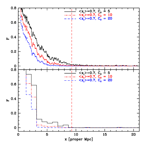
Figure 11.— Sensitivity of mock spectra to clumping in the IGM. Top panel: The solid lines show the transmission averaged over an ensemble of $100$ mock spectra in models with volume-averaged clumping factors of $C_{V}=5$ (i.e., no sub-grid clumping), $10$ and $20$ (from top-to-bottom, black, red, and blue lines respectively). The vertical red dashed line is the same as in previous plots. Bottom panel: The histograms show a single example spectrum, smoothed as in Fan et al. (2005), drawn from each of the above models. The mock spectra are more sensitive to the level of clumpiness than to the volume-averaged neutral fraction in the IGM (see Figure 8 to see the sensitivity to volume-averaged ionization fraction). Indeed, a model with $C_{V}=10$ and a uniform ionizing background ($\langle x_{i}\rangle=1$) with the same mean intensity ($\langle\Gamma_{\rm HI}\rangle=10^{-13}s^{-1}$) yields a nearly identical ensemble-averaged transmission curve to our corresponding $\langle x_{i}\rangle=0.7$ model.

We show mock spectra drawn from our models with sub-grid clumping in Figure 11. Owing to the increased residual neutral fraction within ionized cells, increasing the amount of small scale structure significantly reduces the transmission through the IGM. The models with sub-grid clumping more closely resemble the highest redshift SDSS quasar spectra from Fan et al. (2006) than the calculations shown in Figure 8. We have also produced a model in which the entire volume is uniformly ionized with $\langle\Gamma_{\rm HI}\rangle=10^{-13}s^{-1}$, and $C_{V}=10$ (not shown in plot), which has a nearly identical average transmission profile to our $\langle x_{i}\rangle=0.7$, $C_{V}=10$ case. There is nothing exotic about this model – we expect this level of clumping from our semi-analytic calculations even after reionization is complete. Our results suggest then that the $z\gtrsim 6.2$ Ly$\alpha$ proximity zone measurements are in fact compatible with a highly ionized IGM as previously suggested by Bolton & Haehnelt (2006) and Maselli et al. (2006).

An important caveat to these results is that here we only (crudely) model the enhanced recombination rate from sub-grid clumping; we ignore that our limited simulation resolution likely underestimates the abundance of rare voids in the baryonic density distribution. This effect goes in the opposite direction of the recombination enhancement discussed here and leads to an underestimate of the transmission. Interestingly, note that since the gas distribution is expected to become more smoothed-out as time elapses after reionization, this effect – while not necessarily the dominant one – tends to imply more absorption the earlier reionization occurs. We defer examining this to future work.

Another interesting feature of our calculations is that the transmission close to the quasar is sensitive to the level of clumpiness in the IGM. Sufficiently near the quasar, the photoionization rate is dominated by the quasar itself, and any galactic component is essentially irrelevant (Figure 6). This means that transmission close to the quasar provides a gauge of small-scale structure in the IGM that is insensitive to the details of the (highly uncertain) ionizing background (Cen & Haiman 2000). Interestingly, the transmission profiles near quasars appear to evolve rapidly with redshift around $z\sim 6.2$ (Figure 14 of Fan et al. 2006), possibly a reflection of increased clumpiness in the IGM at high redshifts. Since, given the quasar luminosity, one knows $\Gamma_{\rm HI}$ close to the quasar, one might use this region to calibrate the relation between photoionization rate and transmitted flux. In doing so, one may need to include the impact of quasar overdensities and infall, however (Faucher-Giguére et al. 2007), and account for uncertainties in the quasar ionizing luminosity (Telfer et al. 2002).

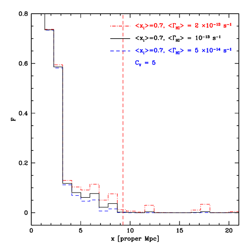
Figure 12.— Sensitivity of mock spectra to the volume-averaged, ‘background’ hydrogen photoionization rate. The precise value of the background hydrogen photoionization rate is affected by several details of our modeling. The histograms show how mock absorption spectra vary in our $\langle x_{i}\rangle=0.7$ case with varying $\langle\Gamma_{\rm HI}\rangle$, assuming no sub-grid clumping ($C_{V}=5$). The transmission profiles are impacted at relatively small distances ($r\sim 5$ proper Mpc) in this example, owing to an upward fluctuation in the galactic photoionization rate.

As mentioned in §4, even for a given model of bubble sizes, there is considerable uncertainty in the precise galactic HI photoionization rate within the ionized bubbles (see Equation 6). This impacts the mock absorption spectra far from the quasar, where photoionization from galactic sources is not overwhelmed by that from the quasar itself. This is in contrast to the influence of sub-grid clumping which, at least in our simplified model, impacts the transmission even near the quasar. In order to illustrate this, we vary the volume-averaged HI photoionization rate around our fiducial value, redo our 1D radiative transfer calculations, and construct new mock spectra. The results of this calculation are shown in Figure 12.

Indeed, boosting the mean intensity of the photoionizing background by a factor of $\sim 2$ increases the transmission far from the quasar noticeably. Note however that if the IGM is more clumpy than in our simulation, as we expect from our arguments above, a still larger $\langle\Gamma_{\rm HI}\rangle$ may be required to achieve this much transmission. On the other hand, diminishing the background intensity by just a factor of $\sim 2$ basically erases the transmission ‘spikes’ far from the quasar. Note that this has little to do with the proximity zone itself – changing the photoionizing background does not impact absorption spectra where the quasar itself dominates the photoionizing flux – and the effect is maximized far from the quasar where the photoionization from galactic sources dominates. This just illustrates the usual sensitivity of absorption spectra to the mean photoionization rate, except here we adopt a more realistic model for the fluctuations in the photoionizing background. In principle, we can constrain our model for the ionizing sources, bubble size distribution, and mean-free path to ionizing photons with these measurements: some of our models may overproduce these transmission spikes compared to the data. In detail, this will require a better handle on the gas density distribution in the IGM, and on our models for sub-grid clumping.

Based on our Figures 11 and 12, it seems plausible that the strong redshift evolution in proximity zone sizes observed by Fan et al. (2006) (their Figure 14) near $z\sim 6.2$ reflects evolution in the level of small scale structure in the IGM, the abundance of rare voids in the gas density distribution, the intensity of the ionizing background, and the cosmic mean gas density, rather than redshift evolution in the volume-weighted ionization fraction. At this point our models are perhaps too crude to warrant a detailed comparison. We intend to return to this issue in future work.

5.4. The Impact of Lyman-limit Systems

In our previous calculations, quasar photons ionize gas at very large distances along some lines of sight, $r\gtrsim 15-20$ proper Mpc. Should we really expect quasars to impact the ionization state of gas at such large distances? The main concern here is that numerical simulations under-produce Lyman limit systems owing to inadequate resolution and missing physics (Miralda-Escudé et al. 1996, Katz et al. 1996, Gardner et al. 1997, Meiksin & White 2004, McDonald et al. 2005b, Kohler & Gnedin 2007, Nagamine et al. 2004, 2007). These studies have focused on $z\sim 3$, but this is likely even more of an issue at $z\sim 6$, especially if some ‘mini-halos’ manage to survive photo-evaporative processes. Missing Lyman-limit systems may impact our results in several ways: first, pre-quasar HII regions will be smaller at a given ionization fraction (Furlanetto & Oh 2005, McQuinn et al. 2006b); second, quasar ionizing photons will propagate less far; and finally, these dense absorbers may leave their imprint on Ly-$\alpha$ absorption spectra. Note that these effects are not well-captured by the clumping-factor approach of the previous section, which is more appropriate for ‘diffuse’ gas in the IGM (Furlanetto & Oh 2005, McQuinn et al. 2006a).

Let us begin by asking the question: how large should we expect the mean free path for ionizing photons to be at $z\sim 6$? (For closely related calculations, see the Appendix of Furlanetto & Oh 2005.) Here, we take an empirically-motivated approach and estimate the mean free path of quasar ionizing photons from the observed column-density distribution in the $z\sim 3$ Ly-$\alpha$ forest, and extrapolate this result to higher redshifts. These quantities are very uncertain even at $z\sim 3$. At $z\sim 3$ the essential difficulty is that absorption systems on the flat part of the curve of growth, where it is difficult to accurately determine column densities, contribute significantly to the effective optical depth for ionizing photons (see, e.g., Meiksin & Madau 1993). Owing to large amounts of saturated absorption in high redshift quasar spectra, the column density distribution is still more uncertain at high redshifts ($z\gtrsim 5$), where Lyman-limit systems cannot be directly identified. Moreover, one might object that the relevant calculation is the mean free path of ionizing photons in the overdense environment of a quasar host halo, with gas subjected to the enhanced ionization field from the quasar, while we will calculate only the mean free path derived from column density distributions measured in typical regions of the IGM.

These objections are correct in detail, but our ensuing calculations should nonetheless provide useful estimates. The mean free path can be calculated from the observed column density distribution of Ly$\alpha$ absorbers, assuming they are Poisson distributed. In this case, the effective optical depth to photons at the ionization edge is given by (see e.g., Zuo & Phinney 1993):

$$\tau_{\rm eff}(\lambda=912\mbox{ \AA},z_{\rm min},z_{\rm max})=\int_{z_{\rm min}}^{z_{\rm max}}dz\times$$

$$\int dN_{\rm HI}f(N_{\rm HI},z)\left(1-e^{-N_{\rm HI}\sigma_{\rm HI}}\right).$$ (7)

The mean free path is then determined by the redshift extent, $z_{\rm max}-z_{\rm min}$, over which $\tau_{\rm eff}=1$. The quantity $f(N_{\rm HI},z)$ represents the column density distribution. The mean free path for higher energy photons is naturally longer, although it scales less rapidly with frequency than in a homogeneous IGM, where one expects $\lambda\propto\nu^{3}$. For example, in the toy case that the column density distribution follows a power law relation, $f(N_{\rm HI})\propto N_{\rm HI}^{-3/2}$, out to arbitrarily large column densities, the mean free path scales as $\lambda\propto\nu^{3/2}$ (Zuo & Phinney 1993). Note that in Equation (7) we include both the residual opacity from the diffuse, ionized IGM (which is presumably incorporated in our calculations), and the opacity from Lyman-limit systems, which is poorly-captured in our simulations.

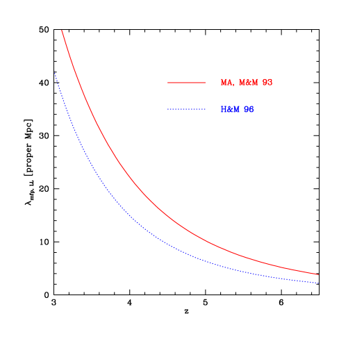
Figure 13.— Mean free path for hydrogen ionizing photons. The curves indicate the proper mean free path of ionizing photons at the Lyman-limit frequency as a function of redshift, derived from two different models for the column-density distribution in the Ly-$\alpha$ forest, extrapolated to high redshift. The red curve adopts the Medium Attenuation model of Meiksin $\&$ Madau (1993), while the blue dotted curve assumes the model of Haardt $\&$ Madau (1996). For both models, the mean free path of Lyman limit photons is $r\lesssim 5$ proper Mpc by $z\sim 6$.

We calculate the mean free path from Equation (7) using two different parameterizations for the observed column density distribution. Specifically, we consider the Medium Attenuation model of Meiksin & Madau (1993), and the model from Haardt & Madau (1996). The differences between these models reflect uncertainties in measurements of the column density distribution. We simply assume the redshift scalings in these parameterized models, based on observations at $z\sim 2-4$, apply even out to $z\sim 6$. The results of this calculation are shown in Figure 13.

In the Haardt & Madau (1996) model, the mean free path for ionizing photons at the Lyman-limit frequency is only $\lambda\sim 3$ proper Mpc at $z\sim 6$, and in the Meiksin & Madau (1993) model the mean free path is only $\lambda\sim 5$ proper Mpc by $z=6$. Higher energy photons have longer mean free paths as described previously. Note that Fan et al. (2002, 2006) estimate the mean free path at $z\sim 6$ directly from absorption spectra data. These inferences are model dependent, but suggest still shorter mean free paths than our extrapolations. Low-column density systems and dense absorbers ($N_{\rm HI}\gtrsim 10^{17}\rm{cm}^{-2}$) provide comparable contributions to the net opacity for Lyman-limit photons. For comparison, quasar photons at the Lyman-limit in our 1D radiative transfer calculations have a mean free path of $\lambda\gtrsim 10$ proper Mpc (once the IGM is ionized – i.e., this mean free path is set by the opacity from residual neutral material along a sightline).

These calculations suggest that our 1D calculations overestimate the mean-free path of Lyman limit photons by a factor of at least $\sim 2$. Note that a Lyman-limit system with $N_{\rm HI}\sim 10^{17}\rm{cm}^{-2}$, by definition, produces an opacity of only $\tau\sim 1$ and hence should attenuate impinging quasar flux, without entirely halting the quasar ionization front. Nevertheless, our estimates suggest that even if the entire volume of the IGM is ionized, we may easily be overestimating the quasar flux at $r\sim 10$ proper Mpc by a factor of $e$ or $e^{2}$. As emphasized previously, reducing the quasar flux by even a factor of a few should lead to significantly more Ly-$\alpha$ absorption and make it harder to distinguish a partly neutral from a fully-ionized IGM on the basis of Ly-$\alpha$ absorption spectra. Crossing a dense absorber will lead to a Lyman-limit absorption system in a Ly-$\alpha$ forest spectrum, but this will be hard to distinguish sufficiently far from the quasar where the typical level of absorption is large.

6. Conclusions

In this paper we argued that, even if the $z\sim 6$ SDSS quasars form when the IGM is partly neutral, they are likely born into large HII regions (see also Yu & Lu 2005). On spherical average, the ionization fraction approaches the global mean after averaging over $R\sim 20-30$ co-moving Mpc/$h$. Nonetheless, much longer skewers towards quasar host halos pass entirely, or predominantly, through ionized bubbles. These effects allow quasar fronts to travel further than expected in a uniformly-ionized medium of the same ionized fraction. We find that the presence of large galaxy-created HII bubbles in patchy reionization models leads to a significant sightline-to-sightline scatter in the extent of quasar ionization fronts. This complicates distinguishing models on the basis of their observed proximity zones. Our results also contradict the expectation for quasar fronts propagating into a homogeneous IGM, in which case front position scales with neutral fraction simply as $R_{s}\propto X_{\rm HI}^{-1/3}$.

We emphasized that the resulting quasar absorption spectra are rather sensitive to uncertainties in the level of small scale structure in the IGM, which impact the mapping between photoionization rate and transmission. In accord with several previous studies (Fan et al. 2006, Bolton & Haehnelt 2006, Maselli et al. 2006), we find that transmission profiles around the $z\sim 6$ SDSS quasars do not generally reveal the extent of quasar ionization fronts. The transmission simply falls close to zero when the combined radiation from the quasar and background galaxies is low enough – essentially, the usual problem that small residual neutral fractions lead to complete absorption in Ly$\alpha$ at high redshift (see also Mesinger & Haiman 2004). The precise neutral fraction at which complete absorption occurs, and the resulting absorption spectra, are sensitive to the level of small scale structure in the IGM, the abundance of rare voids in the IGM, the mean-free path of ionizing photons in the IGM, and the precise photoionization rate within ionized bubbles.

Consequently, we encourage further theoretical study regarding the detailed gas density distribution in the IGM (Miralda-Escudé et al. 2000) and sub-grid clumping factor prescriptions (e.g. Kohler et al. 2005, Trac & Cen 2006). These models can be constrained by comparing with measurements of the one-point probability distribution function in the $z\gtrsim 5$ Ly-$\alpha$ forest (Becker et al. 2006a), by examining the region in the Ly$\alpha$ forest where the photoionization rate is dominated by the quasar itself (see §5.3, Cen & Haiman 2000), and through other measures. These studies should be very useful for improved theoretical modeling of $z\sim 6$ quasar proximity zones, and allow more definitive constraints on the volume-filling factor of HII regions near $z\sim 6$. It might also be interesting to investigate Ly$\beta$ absorption in the proximity zone (Mesinger & Haiman 2004, Bolton & Haehnelt 2006), and other methods of identifying or constraining the presence of damping wing absorption in the observed spectra (Mesinger & Haiman 2006).

There are a few other additional uncertainties that warrant further attention. First, the quasar lifetime is very uncertain observationally. Moreover, the ‘light bulb’ model adopted here in which the quasar radiates at a fixed luminosity for its entire lifetime is likely too simplistic (Hopkins et al. 2005, 2006). It might be interesting to use the $z\sim 6$ black-hole growth simulations of Li et al. (2006), to provide a more realistic description of high redshift quasar life cycles. Observationally, uncertainties in quasar redshifts may be significant (e.g. Shen et al. 2007) and impact proximity zone measurements. Moreover, uncertainties from continuum-fitting – particularly close to the quasar Ly$\alpha$ emission line – warrant further investigation.

We mention several possible future research directions. First, many of the constraints on the $z\sim 6$ IGM adopt a simple model – where one assumes a homogeneous photoionizing background, a uniform temperature-density relation, and that the baryonic distribution is uniformly Jeans-smoothed – which, while remarkably successful at $z\sim 3$ (e.g. McDonald et al. 2005b, Viel & Haehnelt 2006), should break down close to reionization. Demonstrating that this model definitively fails at $z\sim 6$, and identifying which features of the model break, would clearly strengthen the case for reionization activity near $z\sim 6$. On the other hand, the detailed large scale reionization simulations that have been done to date and compared with quasar absorption spectra (e.g. Kohler et al. 2005) have focused on only a single model. It is hard to determine how well alternate models, in which reionization is more or less progressed, would match observations. Indeed, current measurements appear surprisingly consistent with the simple assumption of a spatially uniform ionizing background (Lidz et al. 2006a, Liu et al. 2006). It would be interesting to examine whether highly patchy reionization might overproduce the sightline-to-sightline scatter in the mean absorption. Also, there are certainly dark gaps in the spectra of $z\sim 5.5$ quasars: are we sure of the conventional wisdom that the entire volume of the IGM is ionized by $z\sim 5.5$? The current line of argument for $\langle x_{i}\rangle=1$ at $z\sim 5.5$ comes from assuming a uniform $\Gamma_{\rm HI}$, and finding that a large photoionization rate is required to match the mean transmission in the forest – but this model may lead to misleading conclusions, as one generally expects transmission in the large ionized bubbles that may exist before reionization completes (Furlanetto et al. 2006b). The abundance of dark gaps in $z\sim 6$ quasar spectra is a particularly interesting diagnostic for future modeling (Fan et al. 2002, Lidz et al. 2002, Nusser et al. 2002, Gallerani et al. 2006, Fan et al. 2006).

We also intend to consider 21 cm imaging of quasar HII regions (Madau et al. 1997, Wyithe et al. 2005b). Here, one attempts to detect quasar HII regions based on the brightness temperature contrast between ionized gas around a known quasar and surrounding neutral gas. It would be interesting to investigate whether surrounding galaxy-generated HII regions complicate the morphology of these holes in the 21 cm sky.

Although we have focused on subtleties and challenges associated with interpreting quasar absorption spectra at $z\sim 6$, we should reiterate that they currently provide our most extensive data set regarding the high redshift IGM. Moreover, the rapid redshift evolution seen by Fan et al. (2006) in most of the statistical properties of the $z\sim 6$ Ly$\alpha$ forest is certainly striking, even if the precise theoretical implications are unclear. We believe that future modeling, along the lines mentioned above, should help us understand the ionization state of the IGM at $z\sim 6$ and establish more definitive predictions for future surveys of the high redshift IGM.

References

- (1) Abel, T. & Haehnelt, M. G., 1999, ApJL, 520, 13
- (2) Abel, T., & Wandelt, B. D. 2002, MNRAS, 330, 53
- (3) Barkana, R., & Loeb, A. 2001, Phys. Rept., 349, 125
- (4) Barkana, R., & Loeb, A. 2004, ApJ, 601, 64
- (5) Barkana, R. 2004, MNRAS, 347, 57
- (6) Barth, A. J., Martini, P., Nelson, C. H., & Ho, L. C. 2003, ApJL, 594, L95
- (7) Barton, E. J., Davé, R., Smith, J. T. D., Papovich, C., Hernquist, L., & Springel, V. 2004, ApJL, 604, 1
- (8) Becker, G. D., Rauch, M., & Sargent, W. L. W. 2006a, ApJ submitted, astro-ph/0607633
- (9) Becker, G. D., Sargent, W. L. W., Rauch, M., & Simcoe, R. A. 2006b, ApJ, 640, 69
- (10) Bolton, J. S., & Haehnelt, M. G. 2006, MNRAS in press, astro-ph/0607331
- Bond et al. (1991) Bond, J. R., Cole, S., Efstathiou, G., & Kaiser, N. 1991, ApJ, 379, 440
- (12) Bromm, V., Kudritzki, R. P., & Loeb, A. 2001, ApJ, 552, 464
- (13) Cen, R., & Haiman, Z. 2000, ApJL, 542, 75
- (14) Cen, R., & McDonald, P. 2002, ApJ, 570, 457
- (15) Ciardi, B., Ferrara, A., & White, S. D. M. 2003, MNRAS, 344, L7
- (16) Cohn, J. D., & Chang, T.-C. 2006, MNRAS submitted, astro-ph/0603438
- (17) Dijkstra, M., Haiman, Z., Rees, M. J., & Weinberg, D. H. 2004, ApJ, 601, 666
- (18) Dijkstra, M., Wyithe, J. S. B., & Haiman, Z. 2006, MNRAS submitted, astro-ph/0611195
- (19) Fan, X. et al. 2001, AJ, 122, 2833
- (20) Fan, X. et al. 2002, AJ, 123, 1247
- (21) Fan, X. et al. 2006, AJ, 132, 117
- (22) Faucher-Giguére, C.-A., Lidz, A., Hernquist, L., & Zaldarriaga, M. 2007, ApJ submitted, astro-ph/0701042
- (23) Furlanetto, S. R., Zaldarriaga, M., & Hernquist, L. 2004a, ApJ, 613, 1
- (24) Furlanetto, S. R., Zaldarriaga, M., & Hernquist, L. 2004b, MNRAS, 354, 695
- (25) Furlanetto, S. R., Sokasian, A. & Hernquist, L. 2004c, MNRAS, 347, 187
- (26) Furlanetto, S. R., & Oh, S. P., 2005, MNRAS, 363, 1031
- (27) Furlanetto, S. R., Oh, S. P., & Briggs, F. 2006a, Phys. Reports in press, astro-ph/0608032
- (28) Furlanetto, S. R., Zaldarriaga, M., & Hernquist, L. 2006b, MNRAS, 365, 1012
- (29) Furlanetto, S. R., McQuinn, M., & Hernquist, L. 2006c, MNRAS, 365, 115
- (30) Gallerani, S., Choudhury, T. R., & Ferrara, A. 2006, MNRAS, 370, 1401
- (31) Gardner, J. P., Katz, N., Hernquist, L., Weinberg, D. H., 1997, ApJ, 484, 31
- (32) Gnedin, N. Y., & Hui, L. 1998, MNRAS, 296, 44
- (33) Gunn, J. E., & Peterson, B. A. 1965, ApJ, 142, 1633
- (34) Haiman, Z., & Spaans, M. 1999, ApJ, 518, 138
- (35) Haiman, Z., & Loeb, A. 2001, ApJ, 552, 459
- (36) Haiman, Z., & Holder, G. P. 2003, ApJ, 595, 1
- (37) Haiman, Z., & Cen, R. 2005, ApJ, 623, 627
- (38) Haardt, F., & Madau, P. 1996, ApJ, 461, 20 (HM96)
- (39) Heitmann, K., Lukic, Z., Habib, S., & Ricker, P. M. 2006, ApJL, 642, 85
- (40) Hernquist, L., Katz, N., Weinberg, D.H., & Miralda-Escudé, J. 1996, ApJ, 457, L51
- (41) Hopkins, P. F., Hernquist, L., Martini, P., Cox, T. J., Robertson, B., Di Matteo, T., & Springel, V. 2005, ApJL, 625, 71
- (42) Hopkins, P. F., Hernquist, L., Cox, T. J., Robertson, B., Di Matteo, T., & Springel, V. 2006, ApJS, 163, 1
- (43) Hopkins, P. F., Richards, G.T. & Hernquist, L., 2007, ApJ, 654, 731
- (44) Hui, L., & Gnedin, N. 1997, MNRAS, 292, 27
- (45) Hui, L., Gnedin, N., & Zhang, Y. 1997, ApJ, 486, 599
- (46) Iliev, I. T., Mellema, G., Pen, U., Merz, H., Shapiro, P. R., & Alvarez, M. A. 2006, MNRAS, 369, 1625
- (47) Kaplinghat, M., Chu, M., Haiman, Z., Holder, G. P., Knox, L., & Skordis, C. 2003, ApJ, 583, 24
- (48) Kaiser, N., & Peacock, J. A. 1991, ApJ, 379, 482
- (49) Katz, N., Weinberg, D.H., Hernquist, L. & Miralda-Escudé, J. 1996, ApJ, 457, L57
- (50) Kohler, K., Gnedin, N. Y., & Hamilton, A. J. S. 2005, ApJ submitted, astro-ph/0511627
- (51) Kohler, K., & Gnedin, N. Y. 2007, ApJ, 655, 685
- (52) Li, Y. et al. 2006, ApJ submitted, astro-ph/0608190
- (53) Lidz, A., Hui, L., Zaldarriaga, M., & Scoccimarro, R. 2002, ApJ, 579, 491
- (54) Lidz, A., Oh, S. P., & Furlanetto, S. R. 2006a, ApJL, 639, 47
- (55) Lidz, A., Zahn, O., McQuinn, M., Zaldarriaga, M., Dutta, S., & Hernquist, L. 2006b, ApJ in press, astro-ph/0610054
- (56) Liu, J., Bi, H., Feng, L. L., & Fang, L. Z. 2006, ApJL in press, astro-ph/0605614
- (57) Loeb, A., & Eisenstein, D. J. 1995, ApJ, 448, 17
- (58) Loeb, A., SAAS Winter School (to be published by Springer Verlag), astro-ph/0603360
- (59) Lukic, Z., Heitmann, K., Habib, S., Bashinsky, S., & Ricker, P. M. 2007, ApJ submitted, astro-ph/0702360
- (60) Madau, P., Meiksin, A., & Rees, M. J. 1997, ApJ, 475, 429
- (61) Malhotra, S., & Rhoads, J. 2005, ApJL submitted, astro-ph/0511196
- (62) Martini, P, 2004, in Carnegie Obs. Astrophys. Ser. 1., Coevolution of Black Holes and Galaxies, ed. L. C. Ho (Cambridge: Cambridge Univ. Press), 170, astro-ph/0304009
- (63) Maselli, A., Gallerani, S., Ferrara, A., Choudhury, T. R. 2006, MNRAS submitted, astro-ph/0608209
- (64) McDonald, P. et al. 2005a, ApJ, 635, 761
- (65) McDonald, P., Seljak, U., Cen, R., Bode, P., & Ostriker, J. P. 2005b, MNRAS, 360, 1471
- (66) McQuinn, M., Furlanetto, S. R., Hernquist, L., Zahn, O., & Zaldarriaga, M. 2005, ApJ, 630, 643
- (67) McQuinn, M., Lidz, A., Zahn, O., Dutta, S., Hernquist, L., & Zaldarriaga, M. 2006a, MNRAS submitted, astro-ph/0610094
- (68) McQuinn, M., Zahn, O., Zaldarriaga, M., Hernquist, L., & Furlanetto, S. R. 2006b, ApJ, 653, 815
- (69) Meiksin, A. & Madau, P. 1993, ApJ, 412, 34
- (70) Meiksin, A. & White, M. 2004, MNRAS, 350, 1107
- (71) Mellema, G., Iliev, I. T., Alvarez, M. A., & Shapiro, P. R. 2006a, NewA, 11, 374
- (72) Mellema, G., Iliev, I. T., Pen, U., & Shapiro, P. R. 2006b, MNRAS, 372, 679
- (73) Mesinger, A., & Haiman, Z. 2004, ApJL, 611, 69
- (74) Mesinger, A., & Haiman, Z. 2006, ApJ submitted, astro-ph/0610258
- (75) Miralda-Escudé, J., Cen, R., Ostriker, J. P., Rauch, M., 1996, ApJ, 471, 582
- (76) Miralda-Escudé, J. 1998, ApJ, 501, 15
- (77) Miralda-Escudé, J., Haehnelt, M., & Rees, M. J. 2000, ApJ, 530, 1
- (78) Nagamine, K., Springel, V. & Hernquist, L. 2004, MNRAS, 348, 421
- (79) Nagamine, K., Wolfe, A.M., Hernquist, L. & Springel, V. 2007, ApJ, in press [astro-ph/0510729]
- (80) Navarro, J. F., & Steinmetz, M. 1997, ApJ, 478, 13
- (81) Nusser, A., Benson, A., Sugiyama, N., & Lacey, C. 2002, ApJL, 580, 93
- (82) Oh, S. P. 2002, MNRAS, 336, 1021
- (83) Oh, S. P., & Furlanetto, S. R., 2005, ApJL, 620, 9
- (84) Page, L. et al. 2006, ApJ submitted, astro-ph/0603450
- (85) Peacock, J. A., & Dodds, S. J. 1996, MNRAS, 280, 19
- (86) Press, W. H., & Schechter, P. 1974, ApJ, 187, 425
- (87) Reed, D. et al. 2003, MNRAS, 346, 565
- (88) Ryan-Weber, E. V., Pettini, M., & Madau, P. 2006, MNRAS, 371, L78
- (89) Salpeter, E. E. 1964, ApJ, 140, 796
- (90) Shapiro, P. R., Iliev, I. T., & Raga, A. C. 2004, MNRAS, 348, 753
- (91) Shen, Y. et al. 2007, AJ in press, astro-ph/0702214
- (92) Sheth, R. K., & Tormen, G. 1999, MNRAS, 308, 199
- (93) Shull, J. M. 2004, astro-ph/0410189
- (94) Sokasian, A., Abel, T., & Hernquist, L. 2001, NewA, 6, 359
- (95) Sokasian, A., Abel, T., Hernquist, L., & Springel, V. 2003, MNRAS, 344, 607
- (96) Sokasian, A., Yoshida, N., Abel, T., Hernquist, L., & Springel, V. 2004, MNRAS, 350, 47
- (97) Spergel, D. N. et al. 2006, ApJ submitted, astro-ph/0603449
- (98) Springel, V., & Hernquist, L. 2003, MNRAS, 339, 312
- (99) Springel, V., Di Matteo, T., & Hernquist, L. 2005, MNRAS, 361, 776
- (100) Springel, V. 2005, MNRAS, 364, 1105
- (101) Telfer, R. C., Zheng, W., Kriss, G. A., & Davidsen, A. F. 2002, ApJ, 565, 773
- (102) Thoul, A. A., & Weinberg, D. H. 1996, ApJ, 465, 608
- (103) Totani, T. et al. 2006, PASJ in press, astro-ph/0512154
- (104) Trac, H., & Cen, R. 2006, ApJ submitted, astro-ph/0612406
- (105) Viel, M., & Haehnelt, M. G. 2006, MNRAS, 365, 231
- (106) Wyithe, J. S. B., & Loeb, A. 2004, Nature, 427, 815
- (107) Wyithe, J. S. B., & Loeb, A. 2005, ApJ submitted, astro-ph/0508604
- (108) Wyithe, J. S. B., Loeb, A., & Carilli, C. 2005a, ApJ, 628, 575
- (109) Wyithe, J. S. B., Loeb, A., & Barnes, D. 2005b, ApJ, 634, 715
- (110) Wyithe, J. S. B., & Loeb, A. 2006a, MNRAS submitted, astro-ph/0607246
- (111) Wyithe, J. S. B., & Loeb, A. 2006b, MNRAS submitted, astro-ph/0609734
- (112) Yu, Q., & Lu, Y. 2005, ApJ, 620, 31
- (113) Zahn, O., Zaldarriaga, M., Hernquist, L., McQuinn, M. 2005, ApJ, 630, 657
- (114) Zahn, O., Lidz, A., McQuinn, M., Dutta, S., Hernquist, L., Zaldarriaga, M., & Furlanetto, S. R. 2006, ApJ in press, astro-ph/0604177
- (115) Zaldarriaga, M. 1997, Phys. Rev. D, 55, 1822
- (116) Zaldarriaga, M., Furlanetto, S. R., & Hernquist, L. 2004, ApJ, 608, 622
- (117) Zuo, L. 1992, MNRAS, 258, 36
- (118) Zuo, L. & Phinney, E. S., 1993, ApJ, 418, 28