Introduction to stellar coronagraphy

Abstract

This paper gives a simple and original presentation of various coronagraphs inherited from the Lyot coronagraph. We first present the Lyot and Roddier phase mask coronagraphs and study their properties as a function of the focal mask size. We show that the Roddier phase mask can be used to produce an apodization for the star. Optimal coronagraphy can be obtained from two main approaches, using prolate spheroidal pupil apodization and a finite-size focal mask, or using a clear aperture and an infinite mask of variable transmission.

1 Introduction

Direct imaging of faint companions or planets around a bright star is a very difficult task, where the contrast ratio and the angular separation are the observable parameters. The problem consists of detecting a faint source over a bright and noisy background, mainly due to the diffracted stellar light. High contrast ratios and small angular separations correspond to the most difficult case. Typically, for giant exoplanets, contrast ratios of about $10^{-7}$ are expected in the near infrared (J;H;K bands), based on models for relatively young objects of about 100 Myr [7, 4, 6]. According to these models, older objects would be an order of magnitude fainter. Terrestrial planets are much fainter than giant planets, about 3 to 4 orders magnitudes fainter depending on the wavelength range.

The aim of this article is to give a short review of basic concepts and techniques used in focal plane mask coronagraphy for exoplanets detection. The paper will focus on derivation of a general formalism which allows to gain deeper insight in the behaviour of the principal coronagraphic techniques. It will not consider important problems related for example to the effects of adaptive optics residual speckles, slow-varying speckles caused by mechanical or thermal deformations, telescope central obstruction, chromaticity.

2 Coronagraph general formalism

A common formalism can be used for Lyot and Roddier & Roddier coronagraphs [15, 19] in their classical or apodized version [3, 23, 22], four quadrants coronagraph (4QC) [20], band-limited mask coronagraph [14] and shaped pupil coronagraph [12].

We will follow the notations of [3]. The successive planes of the coronagraph are denoted by $A$, $B$, $C$ and $D$. $A$ is the entrance aperture, $B$ denotes the focal plane with the image mask, $C$ is the image of the aperture with the Lyot stop and $D$ is the image in the focal plane after the coronagraph. The general setup is illustrated in figure 1. The position vector in each plane of the coronagraph will be noted in bold.

• We denote by $p(\vec{x})$ the telescope pupil and $a(\vec{x})$ its possible transmission if a pupil apodization is used. We assume that $\vec{x}$ in $A$ is in units of wavelength.

• The mask transmission is $t(\vec{x})$. We will consider without loss of generality that $t(\vec{x})=1-m(\vec{x})$. The units for the coordinates in $B$ and $D$ are angles on the sky.

• The Lyot stop, denoted as $p_{s}(\vec{x})$ will clearly acts as a low pass filter and consequently its size will be chosen at most equal to the size of the entrance pupil so that $p_{s}(\vec{x})p(\vec{x})=p_{s}(\vec{x})$.

We denote as $\mathcal{P}$, $\mathcal{S}$ and $\mathcal{M}$ the areas defined by the pupil, the stop and if pertinent the mask. We will make the usual approximations of paraxial optics. Moreover we neglect the quadratic phase terms associated with the propagation of the waves or assume that the optical layout is properly designed to cancel it [1]. The constant propagation terms between the successive planes will be omitted. In this case the coronagraph can be easily described using classical Fourier optics: a Fourier transform exists between each of the four planes.

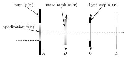
Figure 1: Schematic illustration of Lyot, Roddier & Roddier, 4QC and band-limited mask coronagraph.

The wavefront complex amplitude just before the pupil plane is $\Psi(\vec{x})$. The expression of the complex amplitude in the successive planes $A$, $B$, $C$ and $D$ are:

$$\Psi_{A}(\vec{x}) = \Psi(\vec{x})p(\vec{x})a(\vec{x})$$ (1)

$$\Psi_{B}(\vec{x}) = t(\vec{x})\hat{\Psi}_{A}(\vec{x})=\hat{\Psi}_{A}(\vec{x})-m(\vec{x})\hat{\Psi}_{A}(\vec{x})$$ (2)

$$\Psi_{C}(\vec{x}) = \hat{\Psi}_{B}(\vec{x})p_{s}(\vec{x})=\big{(}\Psi_{A}(\vec{x})-\Psi_{A}(\vec{x})\ast\hat{m}(\vec{x})\big{)}p_{s}(\vec{x})$$ (3)

$$\Psi_{D}(\vec{x}) = \hat{\Psi}_{C}(\vec{x})=\big{(}\hat{\Psi}_{A}(\vec{x})-\hat{\Psi}_{A}(\vec{x})m(x)\big{)}\ast\hat{p}_{s}(\vec{x})$$ (4)

where $\hat{g}$ is the Fourier transform of $g$ and $\ast$ denotes convolution.

The effect of the coronagraph clearly appears in equation (3). The first term is the direct wave diaphragmed by the Lyot stop. The second term corresponds to the wave diffracted by the mask for which the light diffracted outside the aperture in $C$ has been removed. A coronagraph correctly designed for exoplanets imaging can operate one of these two techniques:

1. cancel the on-axis star without altering an off-axis source: for the star the two terms in (3) must interfere destructively whereas for the planet the second term of (3) must cancel. In this case the response of the coronograph is no longer invariant by translation.

2. concentrate the on-axis star light reducing the off-axis diffracted light. This approach corresponds to the apodization techniques [1].

These two techniques can be achieved by a proper choice of the apodization $a(\vec{x})$ and the transmission $t(\vec{x})$. This article will focus on the first solution. For a general overview of pure apodization techniques see [1] and included references.

Section 2 will present the main solutions to this problem that have been derived in the litterature. First the “historical” Lyot coronagraph and the Roddier coronagraph are presented. Whereas the first attempts to cancel the star light, it appears that the second one can also operate by an apodization of the star light. Whereas these coronagraph can provide acceptable results when the dynamic is not too high their performances appear to be insufficient for the detection of earth-like planets. Section 3 addresses the problem of optimal coronagraphy which try to maximize a criterion quantifying the star light rejection. In this context a complete star light rejection can be obtained using an infinite size mask (4QC and band-limited mask) or a finite size $\pi$ phased mask (Roddier coronagraph) with a properly apodized entrance pupil. In the case of a Lyot coronagraph, an apodized aperture allows to maximize the star light rejection for a given mask size. Through all this presentation we will try to be, when possible, as general as possible with respect to the geometry of the system without specializing for example on a specific pupil shape.

3 Lyot and Roddier coronagraphs

The first solution was proposed by Lyot [15] and consists in canceling the major contribution of the star energy located in the telescope point spread function (PSF) inside a disk of radius $r_{m}$. This is simply achieved setting for $t(\vec{x})$ an opaque mask at the center of the image plane $B$.

The results will be presented for a circular aperture of radius $R$ and without central obstruction. The use of polar coordinates will be preferred. Under this asumption $p(\vec{x})=\Pi(r/R)$, $m(\vec{x})=\Pi(r/r_{m})$ and $p_{s}(\vec{x})=\Pi(r/r_{s})$ where $\Pi(r)=1$ for $r\in[0,1)$ and $0$ if $r\geq 1$ and for example: $\hat{p}(\vec{x})=Rr^{-1}J_{1}(2\pi Rr)$. Note that as long as $\Psi_{A}(\vec{x})$, $a(\vec{x})$ and $m(\vec{x})$ are radial functions, the complex amplitudes at the different stages of the coronagraph will exhibit the same symmetry.

Figure 2 illustrates the response of the Lyot coronagraph to an on-axis point source ($\Psi(\vec{x})=1$) for different values of the mask radius $r_{m}$. These values of $r_{m}$ are located on $\hat{\Psi}_{A}(r)$ in figure 3.

We seek to obtain the best subtraction of the two wavefronts $\Psi_{A}(r)$ and $\Psi_{A}(r)\ast\hat{m}(r)$ inside de Lyot stop. Figure 2 cleary shows that this result is achieved increasing the mask size. In fact, as $r_{m}$ increases, $\hat{m}(\vec{x})$ will be more “concentrated” around the origin. As long as $\hat{m}(\vec{x})$ always verifies $\int\hat{m}(\vec{x})d\vec{x}=m(\vec{0})=1$ we have $\hat{m}(\vec{x})\rightarrow\delta(\vec{x})$ as $r_{m}\rightarrow+\infty$, which is the neutral element for the convolution product. On the contrary as $r_{m}$ decreases $\hat{m}(r)$ widens around $\hat{m}(0)=\pi r_{m}^{2}$. At the limit $r_{m}\rightarrow 0$, $\hat{m}(\vec{x})\rightarrow\pi r_{m}^{2}$ and $\Psi_{A}(\vec{x})\ast\hat{m}(\vec{x})$ tends to the constant $\pi^{2}R^{2}r_{m}^{2}$, which does not substract to $\Psi_{A}(\vec{x})=1$. It is interesting to note that this problem is formally equivalent to the problem of digital low-pass filter design with finite impulse response using the windowing method where the infinite impulse response of the ideal filter is truncated using a window, see for example [17].

The results of figure 2 suggest the following comments:

• The performance of the coronagraph is not strictly linear with the mask size. The choice of mask b is as an evidence more appropriate than mask c. This is confirmed by the general shape of the second plot in figure 3 which gives the integrated intensity in $C$ for a Lyot stop of radius $R$.

• A large amount of the residual star energy is located at the edges of the pupil. Consequently a moderate reduction of the diameter of the Lyot stop radius $r_{s}$ will provide a significant gain in starlight rejection with a reasonable loss of transmission. The effect of a Lyot stop reduction is visible in the last two lines of the plot. The value of $r_{s}$ for the last line is indicated in the plots of the intensity in $C$ by a dashed line.

• The off-axis transmission of the coronagraph is of course a crucial point for planet detection. As long as the angular distance from the optical axis is sufficient to guaranty that the response of the planet in $B$ will not interfere with the mask, we can consider that the response of the planet will be the shifted PSF of a pupil with radius $r_{s}$. In order to quantify the loss of transmission for an off-axis source, this PSF has been added in figure 2. Finally, note that a solution to the analytical computation of $\Psi_{C}(r,\theta)$, $\Psi_{D}(r,\theta)$ of a point source which can be close to the optical axis has been addressed in [8].

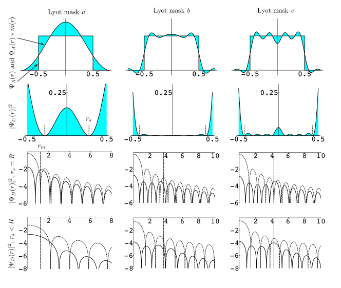
Figure 2: Illustration of Lyot coronagraphy for circular aperture (radial cuts) and an on-axis point source. The first raw represents the two complex amplitudes that should interfere destructively in $C$. The second row gives the intensity in $C$ and the third and fourth raw the intensity in $D$. In the two last rows, the continuous line represents the intensity in $D$ for a coronagraphed point source and the dashed line the PSF associated to a pupil of radius $r_{s}$. The vertical dashed line in the last row indicates the radius of the mask.

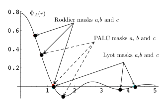
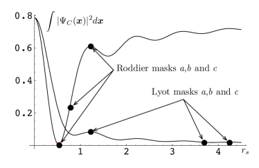
Figure 3: The left plot locates the different masks used in the simulation on the response of an on-axis point source. The right plot gives the integrated intensity in $C$ for $r_{s}=R$ as a function of the mask size.

The Lyot technique was improved by Roddier [19] replacing the opaque mask by a $\pi$ phase mask: $m(\vec{x})=2\Pi(r/r_{m})$. Figure 4 show that for very small values of $r_{m}$, the Roddier coronagraph tends to behave like the Lyot coronagraph, trying to cancel out the light of the star. This behavior totally differs when $r_{m}$ increases: for mask size a or b the effect of this coronagraph is to produce in the plane C an apodized version of the wavefront originated by an on-axis source. Note that a coronagraphic technique relying on a similar principle was proposed in [16] using a $\pi/2$ phase mask and a defocus. The effect of this apodization is visible in D: the main lobe of the response is broadened whereas the side lobes decrease. Moreover, it is worthy to note that this apodization as a maximum value for $\vec{x}=0$ that can be higher than 1.

These results suggest the following comments:

• the choice of $r_{m}$ remains a crucial point. However, according to the preceding remark the integrated energy in C ploted in figure 3 is no more a valid criterion for selection of an optimal value of $r_{m}$.

• As the second row of figure 3 shows, a reduction of the Lyot stop is not crucial as long as the Roddier coronagraph operates in its “ apodization mode”.

• The effect of a Roddier coronagraph on a planet relies on the same principle as the Lyot coronagraph. Consequently the apodization effect mentioned above will not operate for an off-axis source. Moreover, the fact that for this latter coronagraph the mask will be smaller and a reduced stop is not necessary will increase its performances in terms of resolution and planet flux.

According to the previous remarks, a Roddier coronagraph with an extended mask can be used as an apodizer for the wavefront complex amplitude. The star rejection of such a system being insufficient for planet detection such a device should be considered as the first stage of a “classical” coronagraph.

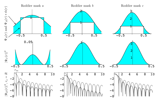
Figure 4: Illustration of Roddier coronagraphy for circular aperture (radial cuts) and an on-axis point source. The first raw represents the two complex amplitudes that should interfere destructively in $C$. The second row gives the intensity in $C$ and the third raw the intensity in $D$. In the last row, the continuous line represents the intensity in $D$ for a coronagraphed point source and the dashed line the PSF associated to a pupil of radius $r_{s}$.

4 Optimal coronagraphy

According to equation (3) the ideal coronagraph equation is:

$$\Psi_{A}(\vec{x})=\Psi_{A}(\vec{x})\ast\hat{m}(\vec{x}),\;\forall\vec{x}\in\mathcal{S}$$ (5)

where $\Psi_{A}(\vec{x})=a(\vec{x})p(\vec{x})$. Following Lyot and Roddier coronagraphs, a first solution is to set $m(r)=\epsilon\Pi(r/r_{m})$ where $\epsilon=1$ for Lyot and $\epsilon=2$ for Roddier and to find, if it exists, the optimal apodization $a(\vec{x})$ solution of the integral equation (5). This solution was first proposed by [5] and [11]. The other solution is to suppress the constraint on the mask and to find the function $m(\vec{x})$ solution of equation (5) when $a(\vec{x})=1$. This approach includes the band-limited masks proposed by [14] and the four quadrants coronagraph [20].

4.1 Finite size masks: apodized Lyot and Roddier coronagraphs

As long as $m(\vec{x})$ has a bounded symmetric support $\mathcal{M}$, we can write using the notations of Apendix B: $\hat{m}(\vec{x})=\epsilon K_{M}(\vec{x})$. Consequently, equation (13) implies that if $a(\vec{x})$ is proportional to a spheroidal prolate function associated to $\mathcal{M}$ and $\mathcal{P}$, the residual in $C$ when $p_{s}(\vec{x})=p(\vec{x})$ is obtained replacing in (3) the second term by $\epsilon\Lambda\Psi_{A}(\vec{x})$:

$$\Psi_{C}(\vec{x})=(1-\epsilon\Lambda)\Psi_{A}(\vec{x})$$ (6)

which states that the residual wavefront in $C$ originated by an on-axis source is proportional to the apodized entrance pupil. If we assume that the angular distance of the planet is sufficient, its response in $C$ is obtained setting $\epsilon=0$ in (6). The tradeoff between the reduction of the planet flux by the apodization and the reduction of the star flux by the coronagraph can be evaluated by the quantity $\eta$ defined as the ratio between the total planet intensity in $D$ and the total star intensity outside the mask in $D$.

From equation (6) the star intensity in $D$ is simply $(1-\epsilon\Lambda)^{2}|\hat{\Psi}_{A}(\vec{x})|^{2}$. The total energy outside the mask is:

$$(1-\epsilon\Lambda)^{2}\big{(}\int_{\mathbb{R}^{2}}|\hat{\Psi}_{A}(\vec{x})|^{2}d\vec{x}-\int_{\mathcal{M}}|\hat{\Psi}_{A}(\vec{x})|^{2}d\vec{x}\big{)}=(1-\epsilon\Lambda)^{2}\big{(}\int_{\mathbb{R}^{2}}|\hat{\Psi}_{A}(\vec{x})|^{2}d\vec{x}-\Lambda\int_{\mathbb{R}^{2}}|\hat{\Psi}_{A}(\vec{x})|^{2}d\vec{x}\big{)}$$ (7)

where the last equality comes from the fact that $\epsilon\Lambda$ is the ratio between the energy encircled in the bounded frequency domain $\mathcal{M}$ and the total energy of $\Psi_{A}(\vec{x})$. As a consequence we have:

$$\eta=(1-\epsilon\Lambda)^{2}(1-\Lambda)$$ (8)

The objective will be to minimize $\eta$ for a given coronagraph type ($\epsilon=1$ or 2). This is achieved by a modification of the size of $\mathcal{M}$ which will affect $\Lambda$ and the pupil apodization shape $a(\vec{x})$.

Any eigenvalue of the integral equation minimizing (8) leads to a valid solution. However we will only consider in the sequel the largest eigenvalue, i.e. corresponding to the maximum encircled energy behind the focal plane mask. This choice will in fact “generally” lead to a positive prolate function which will be normalized by its maximum value on the pupil in order to achieve an apodization with maximum transmission. Finally, it is worthy to note that this development does not require a specific shape of the pupil and the mask. However, further analytical derivations based on equations (14) and (15) require that the mask is a scaled version of the pupil: in this case if the pupil has a central obstruction $m(\vec{x})$ has a hole. This point will not be considered herein.

• We consider first the case of an apodized Roddier coronagraph, $\eta=(1-2\Lambda)^{2}(1-\Lambda)$. The results of Appendix A prove that 1/2 is a valid eigenvalue and consequently a mask size can be chosen to achieve $\eta=0$, i.e. a total extinction of the star.

  For example, in the case of a circular pupil without obstruction, figure 8 shows that the coefficient $c=r_{m}R\approx 0.25$ corresponds to $\Lambda=1/2$. This value defines the apodization shape and fixes the mask size to $r_{m}\approx 0.25/R$. Figure 5 gives the corresponding apodization. This figure also illustrates the loss in transmission for an off axis planet comparing the prolate apodized pupil PSF with the PSF of the unapodized pupil.

• We consider now a prolate apodized Lyot coronagraph (PALC), $\eta=(1-\Lambda)^{3}$. The eigenvalues being upper-bounded by 1, a prolate apodized Lyot coronagraph (PALC) cannot achieve total extinction of an on-axis point source. The trivial solution $\Lambda=1$ would correspond to an infinite size opaque mask. However, approximate solutions can be obtained for eigenvalues $\Lambda$ close to 1 and finite mask size. Taking advantage of the rapid saturation of the eigenvalue curve we can choose a mask size corresponding to an eigenvalue close to 1.

  Figure 6 illustrates the response of the PALC to an on-axis point source for different values of the mask radius $r_{m}$ given in figure 3. To each value of $r_{m}$ corresponds a coefficient $c$ and and optimal apodization function given in the first row. The second row gives the residue in $C$ and the last row the response of the star and the PSF associated to the apodized telescope pupil. Note that contrarily to the unapodized Roddier coronagraph operating in its “apodized regime” (see column 2 and 3 of figure 4) the residue in $C$ is here both apodized and attenuated. An analog comment can be done for the apodization alone coronagraphs.

  The property that the Lyot stop wave amplitude is proportional to the entrance apodized pupil amplitude, creates the possibility for multiple stage coronagraphs described in [2]. A multiple stage PALC only requires a single apodizer in the entrance pupil. The Lyot stop plane is naturally apodized and can be used as the entrance pupil of a second coronagraphic stage without further loss of throughput due to apodization. In this case the residual amplitude in the second Lyot stop plane is $(1-\Lambda)^{2}\Psi_{A}(\vec{x})$ and the parameter $\eta$ becomes $(1-\Lambda)^{5}$.

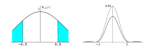
Figure 5: Illustration of Roddier apodized coronagraphy for circular aperture (radial cuts). The left plot shows the optimally prolate apodized pupil. The right plot shows the PSF corresponding to the prolate apodized pupil and the PSF of the unapodized pupil.

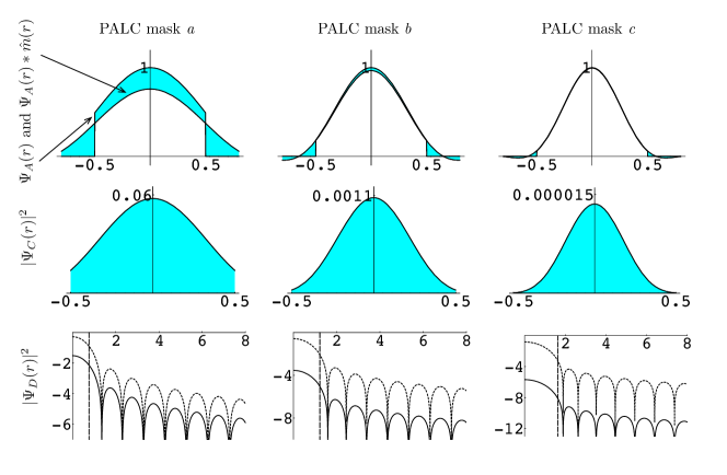
Figure 6: Illustration of prolate apodized coronagraphy for circular aperture (radial cuts) and an on-axis point source. The first raw represents the two complex amplitudes that should interfere destructively in $C$. The second row gives the intensity in $C$ and the third and fourth raw the intensity in $D$. In the last row, the continuous line represents the intensity in $D$ for a coronagraphed point source and the dashed line the PSF associated to the apodized telescope pupil.

4.2 Infinite size masks band limited and four quadrants coronagraphs

A simple solution to define a mask $m(\vec{x})$ that verifies (5) is to chose $m(\vec{x})$ such that $\hat{m}(\vec{x})$ is non zero only on a small bounded region $\mathcal{B}$ included inside the pupil. In this case if we define $\mathcal{S}$ such as $\forall\vec{x}_{0}\in\mathcal{S}$ the support of $\hat{m}(\vec{x}_{0}-\vec{x})$ is strictly included in the pupil $\mathcal{P}$:

$$\forall\vec{x}_{0}\in\mathcal{S},\;\Psi_{A}(\vec{\vec{x}_{0}})\ast\hat{m}(\vec{x}_{0})=\int_{\mathcal{P}}\hat{m}(\vec{x}_{0}-\vec{x})d\vec{x}=m(\vec{0})$$ (9)

Consequently, if we impose $m(\vec{0})=1$ we will clearly verify equation (5) on $\mathcal{S}\subset\mathcal{P}$. Figure 7 illustrates the definition of the various sets $\mathcal{S}$, $\mathcal{P}$ and $\mathcal{B}$. A simple solution to block the residue in $\mathcal{P}\backslash\mathcal{S}$ is to use as a Lyot stop the indicator function of $\mathcal{S}$, $p_{s}(\vec{x})={\mathchoice{\rm 1\mskip-4.0mul}{\rm 1\mskip-4.0mul}{\rm 1\mskip-4.5mul}{\rm 1\mskip-5.0mul}}_{\mathcal{S}}(\vec{x})$ ($p_{s}(\vec{x})=1$ if $\vec{x}\in\mathcal{S}$ and $0$ elsewhere). Consequently a properly defined band limited, and necessary infinite size mask $m(\vec{x})$ must verify: $m(\vec{0})=1$, $0\leq m(\vec{x})\leq 1$ and $m(\vec{x})$ is bandlimited on $\mathcal{B}\subset\mathcal{P}$. This approach was proposed by [13].

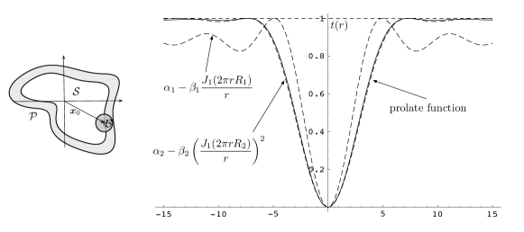
Figure 7: Left figure: relation between the pupil ($\mathcal{P}$), support of the mask Fourier transform ($\mathcal{B}$) and the Lyot stop $\mathcal{S}$ in a bandlimited coronagraph. Right figure: illustration of three different masks. Dashed lines: second and fourth order Bessel cardinal masks. Continuous line: prolate spheroidal function.

A fundamental result for understanding of band limited coronagraphs states that the complex amplitude in $D$ associated to an off-axis point source at an angle $\vec{x}_{1}$ is the response of the Lyot stop attenuated by the transmission at $\vec{x}_{1}$:

$$\Psi_{D}(\vec{x})=t(\vec{x}_{1})\hat{p}_{s}(\vec{x}-\vec{x}_{1})$$ (10)

This result is demonstrated in [13]. This result suggests the following comments:

1. The loss of throughput of a bandlimited coronagraph is principally due to the undersizing of the Lyot stop. Consequently $\mathcal{B}$ should be as small as possible. However the general consequences of a reduction of $\mathcal{B}$ are a widening of the central lobe of $m(\vec{x})$ and an increase of the ripples in the tails of $m(\vec{x})$. From equation (10) the first effect implies an increase of a blind zone arround the star and the second a reduction of detectability for given locations of a planet.

2. The behavior of the coronagraph when the star is slightly off-axis is perfectly described by equation (10): in order to reduce the effect of a misalignmemt $m(\vec{x})$ must be as “flat” as possible in $\vec{0}$. This effect is quantified in [13] by the degree of the first term in the serie expansion of $t(\vec{x})$. Note that the flatness of $m(\vec{x})$ around $\vec{x}=\vec{0}$ is of course deeply related to the constraints previously mentioned. Finally, a technique to construct a mask of given order adding and multiplying simple band-limited masks is proposed in [13].

To conclude, figure 7 compares the behavior of three different radial transmissions in the case of a circular aperture. To facilitate this comparison the three masks have been normalized to the same $\mathcal{B}$ in order to guaranty that the Lyot stop will be the same: for these simulations the flux reduction equals $4/9$. The first transmission is a Bessel cardinal function and the second one the square of a Bessel cardinal function. These functions have been properly scaled and shifted in amplitude in order that $t(r)$ occupies all the interval $[0,1]$. The properties detailed in the item (i) of the discussion above can also be expressed in term of concentration of the energy of $m(\vec{x})$ around the origin. In this case, the additional band-limited constraints leads naturally to a prolate function. Such a solution is illustrated in figure 7. In this case the coefficient $c$ has been chosen empirically equal to 6.8 in order to achieve a good compromise between the the ripples and the width of the main lobe. This result shows that the behavior of such a prolate mask and a squared Bessel cardinal mask are similar. Finally, it is important to emphasize that the masks illustrated in figure 7 correctly behave with respect to the requirement (i). On the contrary they do not fulfil (ii) (the order of the squared Bessel cardinal and the prolate is only 4) and will have a poor behavior in the case of a resolved star or a misalignment.

To conclude, it is important to mention in this section devoted to optimal coronagraphy with infinite size masks the 4QC. This coronagraph will be developed in a separate paper by D. Rouan in this volume. It relies on the fact that for a circular aperture and a transmission $t(\vec{x})=\text{sign}(x)\text{sign}(y)$, the complex amplitude in $C$ is identically zero inside the pupill for a point source on the axis. This beautiful result relies on a nontrivial property of the Fourier transform (see the paper of D. Rouan and included references for a proof). A coronagraphic technique based on a similar principle is developped in [9].

Appendix A Prolate spheroidals functions

This section presents some facts about prolate spheroidals functions. For a detailed presentation refer to the seminal papers [21] and references therein. Application of prolate spheroidals functions to optics can be found in [10].

In order to gain deeper insight in their principal properties using simple mathematics the cartesian coordinates have been prefered. Derivations using specific coordinates can be found in the references. We consider a real valued square-integrable function $f$ of $d$ variables having a bounded support $\mathcal{P}$ (in our case $f(\vec{x})=a(\vec{x})p(\vec{x})$ and $\mathcal{P}$ is the telescope pupil):

$$\hat{f}(\vec{x})=\int_{\mathcal{P}}f(\vec{y})e^{-\imath 2\pi\vec{x}^{t}\vec{y}}d\vec{y}$$ (11)

The ratio between the energy encircled in the bounded frequency domain $\mathcal{M}$ (here the Lyot mask) and the total energy of $\hat{f}$ is obtained integrating the squared modulus of (11) on $\mathcal{M}$:

$$\int_{\mathcal{P}}K_{\mathcal{M}}(\vec{x}-\vec{y})f(\vec{y})f(\vec{x})d\vec{y}d\vec{x}\big{/}\int_{\mathcal{P}}f(\vec{y})^{2}d\vec{y}$$ (12)

where $K_{\mathcal{M}}(\vec{x})$ is the inverse Fourier transform of the indicator function of $\mathcal{M}$, ${\mathchoice{\rm 1\mskip-4.0mul}{\rm 1\mskip-4.0mul}{\rm 1\mskip-4.5mul}{\rm 1\mskip-5.0mul}}_{\mathcal{M}}(\vec{x})$. Standard results on functional analysis, see for example [18], prove that the maximum of this ratio is the largest eigenvalue $\Lambda$ of the integral equation:

$$\int_{\mathcal{P}}K_{\mathcal{M}}(\vec{x}-\vec{y})\psi(\vec{y})d\vec{y}=\Lambda\psi(\vec{x}),\;\vec{x}\in\mathcal{P}$$ (13)

or equivalently: $\big{(}\psi(\vec{x}){\mathchoice{\rm 1\mskip-4.0mul}{\rm 1\mskip-4.0mul}{\rm 1\mskip-4.5mul}{\rm 1\mskip-5.0mul}}_{\mathcal{P}}(\vec{x})\big{)}\ast K_{\mathcal{M}}(\vec{x})=\Lambda\psi(\vec{x})$, $\vec{x}\in\mathcal{P}$.

The prolate spheroidal functions are defined as the solution of this integral equation. The extrema of (12) is reached when $f(\vec{x})$ is the corresponding eigenfunction. The kernel being positive defined the eigenvalues of (13) are positive and from (12) upper bounded by 1. The eigenfunctions of (13) are orthogonal and complete on $L_{2}(\mathcal{P})$ and orthogonal on $\mathbb{R}^{d}$ when extended outside $\mathcal{P}$ using (13).

Considerable simplifications occur when $\mathcal{P}$ and $\mathcal{M}$ are both scaled versions of a “normalized” domain $\mathcal{U}$: $\exists\vec{R}\in\mathbb{R}^{d}$, $\exists\vec{r}_{m}\in\mathbb{R}^{d}$ such that $\vec{x}\in\mathcal{P}\Leftrightarrow\vec{x}./\vec{R}\in\mathcal{U}$, $\vec{x}\in\mathcal{M}\Leftrightarrow\vec{x}./\vec{r}_{m}\in\mathcal{U}$, where $\vec{a}./\vec{b}$ (resp. $\vec{a}.\vec{b}$) defines the vector having $a(k)/b(k)$ (resp. $a(k)b(k)$) as components. A simple change of variable in the definition of $K_{\mathcal{M}}(\vec{x})$ shows that $K_{\mathcal{M}}(\vec{x})=\left(\prod_{k=1}^{d}r_{m}(k)\right)K_{\mathcal{U}}(r_{m}.\vec{x})$. Substitution of this result in (13) shows that $\psi(\vec{x})=\phi(R.\vec{x})$ where $\phi(\vec{x})$ is the solution of the normalized problem:

$$\left(\prod_{k=1}^{d}r_{m}(k)R(k)\right)\int_{\mathcal{U}}K_{\mathcal{U}}(\vec{r}_{m}.\vec{R}.(\vec{x}-\vec{y}))\phi(\vec{y})d\vec{y}=\Lambda\phi(\vec{x}),\;\vec{x}\in\mathcal{U}$$ (14)

• Consider for example the case where $d=2$ and $\mathcal{U}$ is a disk. Consequently $\mathcal{P}$ and $\mathcal{M}$ are ellipses. Equation (14) shows that the prolate functions associated to an ellipse are obtained by a scaling of the prolate function associate to a disk.

• If $\forall k,\;R(k)=R$ and $r_{m}(k)=r_{m}$, equation (14) shows that the prolate spheroidal functions for a given $\mathcal{U}$ form essentially a one-parameter family of functions depending of the parameter $c=r_{m}R$.

Additional simplifications in this last case are obtained when the region $\mathcal{U}$ is symmetric: $\vec{x}\in\mathcal{U}\Leftrightarrow-\vec{x}\in\mathcal{U}$. In this case the solutions of (14) are real, either even with a real eigenvalue or odd with a pure imaginary eigenvalue. Moreover, finding the solutions of (14) is equivalent to finding the solutions of:

$$\alpha\phi(\vec{x})=\int_{\mathcal{U}}e^{-\imath 2\pi c\vec{x}^{t}\vec{y}}\phi(\vec{y})d\vec{y},\;\vec{x}\in\mathcal{U},\;\text{where }\Lambda=|\alpha|^{2}c^{d}$$ (15)

This equation states that the Fourier transform of $\phi(\vec{x}){\mathchoice{\rm 1\mskip-4.0mul}{\rm 1\mskip-4.0mul}{\rm 1\mskip-4.5mul}{\rm 1\mskip-5.0mul}}_{\mathcal{U}}(\vec{x})$ is proportional to $\phi(\vec{x}/c)$. This result can be easily verified taking the complex conjugate of (15), substituting in the integral $\phi(\vec{y})$ by the right side of (15) and identifying with (14).

Circular prolate functions correspond to the case $d=2$ where $\mathcal{U}$ is the unit disk. They decompose, up to a normalisation factor as $\phi_{N,n}(r,\theta)=R_{N,n}(r)[\cos,\sin](N\theta)$. Consequently (15) shows that they can be defined by their invariance to a finite Hankel transform of order $N$, e.g.:

$$2\pi\int_{0}^{1}R_{0,0}(r)J_{0}(2\pi r\rho)rdr=\frac{\sqrt{\Lambda}}{r_{m}}R_{0,0}\left(\frac{\rho}{r_{m}}\right)$$ (16)

Figure 8 represents the radial circular prolate function $\phi_{0,0}(r)$ for three different values of $c$.

A crucial point is the numerical computation of prolate functions. For simple geometries, the functions can be computed using rapidly converging series as the one derived for a circular aperture in [21]. For general geometries, prolate spheroidal functions can be computed directly solving equation (13) using one of the numerous iterative algorithm that can be found in the litterature for the computation of the eigenelements of linear integral operators, e.g. the algorithm used in [11].

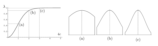
Figure 8: Circular prolate functions. Left plot gives the largest eigenvalue $\Lambda$ as a function of $4c$. The right plot gives the prolate functions for three values of $c$.

References

- Aime [2005] Aime, C., May 2005. Radon approach to shaped and apodized apertures for imaging exoplanets. Astronomy and Astrophysics 434, 785–794.
- Aime and Soummer [2004] Aime, C., Soummer, R., oct 2004. Multiple-stage apodized pupil Lyot coronograph for high contrast imaging. In: Astronomical Telescopes and Instrumentation 2004. SPIE, pp. 456–461.
- Aime et al. [2002] Aime, C., Soummer, R., Ferrari, A., 2002. Total coronographic extinction of rectangular apertures using linear prolate apodizations. Astronomy and Astrophysics 389, 334–344.
- Baraffe et al. [2003] Baraffe, I., Chabrier, G., Barman, T., Allard, F., Hauschildt, P. H., 2003. Evolutionary models for cool brown dwarfs and extrasolar giant planets. the case of hd 20945. Astronomy and Astrophysics 402, 701.
- Baudoz [1999] Baudoz, P., 1999. Imagerie interférométrique grand champ et applications. Thèse de Doctorat, Université Nice Sophia Antipolis.
- Burrows et al. [2004] Burrows, A., Sudarsky, D., Hubeny, I., 2004. Spectra and diagnostics for the direct detection of wide-separation extrasolar giant planets. The Astrophysical Journal 609, 407.
- Chabrier and Baraffe [2000] Chabrier, G., Baraffe, I., 2000. Theory of low-mass stars and substellar objects. Annual Review of Astronomy and Astrophysics 38, 337.
- Ferrari [2007] Ferrari, A., march 2007. Analytical analysis of lyot coronographs response. The Astrophysical Journal 657, 1201.
- Foo et al. [2005] Foo, G., Palacios, D. M., Swartzlander, G. A., dec 2005. Optical vortex coronagraph. Optics Letters 30, 3308–3310.
- Frieden [1971] Frieden, B., 1971. Progress in Optics. North-Holland, Ch. VIII, pp. 311–407.
- Guyon and Roddier [2000] Guyon, O., Roddier, F., 2000. Direct exoplanet imaging possibilities of the nulling stellar coronagraph. In: Interferometry in Optical Astronomy. Vol. 4006. SPIE, pp. 377–387.
- Kasdin et al. [2003] Kasdin, N. J., Vanderbei, R. J., Spergel, D. N., Littman, M. G., jan 2003. Extrasolar planet finding via optimal apodized pupil and shaped-pupil coronagraphs. The Astrophysical Journal 582, 1147—1161.
- Kuchner et al. [2005] Kuchner, M., Crepp, J., Ge, J., 2005. Eighth-order image masks for terrestrial planet finding. The Astrophysical Journal 628, 466–473.
- Kuchner and Traub [2002] Kuchner, M., Traub, W., 2002. A coronagraph with a band-limited mask for finding terrestrial planets. The Astrophysical Journal 570, 900–908.
- Lyot [1939] Lyot, B., 1939. The study of the solar corona and prominences without eclipses (george darwin lecture, 1939). Monthly Notices of the Royal Astronomical Society 99, 580.
- Martinache [2004] Martinache, F., Aug. 2004. PIZZA: a phase-induced zonal zernike apodization designed for stellar coronagraphy. Journal of Optics A: Pure and Applied Optics 6, 809–814.
- Oppenheim and Schafer [1989] Oppenheim, A., Schafer, R., 1989. Discrete-time signal processing. Prentice-Hall, Inc. Upper Saddle River, NJ, USA.
- Riesz and Sz.-Nagy [1990] Riesz, F., Sz.-Nagy, B., 1990. Functional Analysis. Dover Publications.
- Roddier and Roddier [1997] Roddier, F., Roddier, C., 1997. Stellar coronagraph with phase mask. Astronomical Society of the Pacific 109, 815–820.
- Rouan et al. [2000] Rouan, D., Riaud, P., Boccaletti, A., Clénet, Y., Labeyrie, A., 2000. The four-quadrant phase-mask coronagraph I. principle. Publication of the Astronomical Society of the Pacific 112, 1479–1486.
- Slepian [1964] Slepian, D., 1964. Prolate spheroidal wave functions, Fourier analysis and uncertainty, IV : Extensions to many dimensions; generalized prolate spheroidal functions. Bell System Technical Journal 43, 3009–3058.
- Soummer [2004] Soummer, R., 2004. Apodized pupil lyot coronagraphs for arbitrary telescope apertures. The Astrophysical Journal 618, 161–164.
- Soummer et al. [2003] Soummer, R., Aime, C., Falloon, P., 2003. Stellar coronography with prolate apodized circular apertures. Astronomy and Astrophysics 397, 1161–1172.