11email: remo@mpa-garching.mpg.de 22institutetext: Department of Astronomy and Space Physics, Uppsala University, BOX 515, SE–751 20 Uppsala, Sweden
33institutetext: Research School of Astronomy & Astrophysics, Mount Stromlo Observatory, Cotter Road, Weston ACT 2611, Australia
33email: martin@mso.anu.edu.au, art@mso.anu.edu.au
Three-Dimensional Hydrodynamical Simulations of Surface Convection in Red Giant Stars
Abstract
Aims. We investigate the impact of realistic three-dimensional (3D) hydrodynamical model atmospheres of red giant stars at different metallicities on the formation of spectral lines of a number of ions and molecules.
Methods. We carry out realistic, ab initio, 3D, hydrodynamical simulations of surface convection at the surface of red giant stars with varying effective temperatures and metallicities. We use the convection simulations as time-dependent hydrodynamical model stellar atmospheres to calculate spectral lines for a number of atomic (Li i, O i, Na i, Mg i, Ca i, Fe i, and Fe ii) and molecular (CH, NH, and OH) lines under the assumption of local thermodynamic equilibrium (LTE). We carry out a differential comparison of the line strengths computed in 3D with the results of analogous line formation calculations for classical, 1D, hydrostatic, plane-parallel marcs model atmospheres in order to estimate the impact of 3D models on the derivation of elemental abundances.
Results. The temperature and density inhomogeneities and correlated velocity fields in 3D models, as well as the differences between the mean 3D stratifications and corresponding 1D model atmospheres significantly affect the predicted strengths of spectral lines. Under the assumption of LTE, the low atmospheric temperatures encountered in 3D model atmospheres of very metal-poor giant stars cause spectral lines from neutral species and molecules to appear stronger than within the framework of 1D models. As a consequence, elemental abundances derived from these lines using 3D models are significantly lower than according to 1D analyses. In particular, the differences between 3D and 1D abundances of C, N, and O derived from CH, NH, and OH weak low-excitation lines are found to be in the range dex to dex for the the red giant stars at considered here. At this metallicity, large negative corrections (about dex) are also found, in LTE, for weak low-excitation Fe i lines. We caution, however, that the neglected departures from LTE might be significant for these and other elements and comparable to the effects due to stellar granulation.
Key Words.:
Convection – Hydrodynamics – Line: formation – Stars: abundances – Stars: late-type – Stars: atmospheres1 Introduction
Stars in the red giant phase of their evolution are characterized by large stellar diameters and increased luminosities compared with unevolved objects. Because of their high intrinsic brightnesses, red giants represent natural targets for a wide range of observational studies. Stars of this luminosity class are especially suitable for investigations of distant stellar systems in the Milky Way as well as in other galaxies of the Local Group. Giant stars are extensively used in spectroscopic analyses for tracing elemental abundances in distant stellar populations. A significant fraction of the halo and disk stars included in various large-scale stellar abundance analyses (e.g. McWilliam et al. 1995; Ryan et al. 1996; Fulbright 2000) are indeed giants. More recently, the ESO “First Stars” programme (e.g. Hill et al. 2002; Cayrel et al. 2004; Spite et al. 2005) has provided a systematic and homogeneous study of the chemical compositions of a large sample of extremely metal-poor giant as well as dwarf stars () from the HK survey by Beers et al. (1992, 1999). The recently discovered extreme halo star HE (Christlieb et al. 2002), one of the most iron-poor star known to date, is also a giant. Red giants are also used to study Galactic metallicity gradients in the Galactic disk and open clusters (Yong et al. 2005; Carney et al. 2005) and star-to-star elemental abundance variations within globular clusters (for a review, see Gratton et al. 2004). The results of these and similar observational studies provide valuable information about fundamental astrophysical processes and are essential for our understanding of stellar nucleosynthesis and internal mixing as well as Galactic chemical evolution. Accurate determinations of elemental abundances in metal-poor stars and red giants in particular are crucial for deducing the physical and evolutionary properties of the very first generation of stars (Weiss et al. 2004; Iwamoto et al. 2005; Meynet et al. 2006) and distinguishing among the various proposed scenarios of chemical enrichment of the Galaxy.
As for other late-type stars, ordinary classical abundance analyses of red giants involve theoretical 1D model atmospheres constructed under the assumptions of plane-parallel geometry (or spherical symmetry), hydrostatic equilibrium, and flux constancy (e.g. Gustafsson & Jorgensen 1994). The simplifying approximation of LTE is also normally adopted. Furthermore, 1D modelling of stellar atmospheres generally relies on a rudimentary treatment of convective energy transport, such as the mixing length theory (Böhm-Vitense 1958) or one of its derivatives (e.g. Canuto & Mazzitelli 1991), all dependent on a number of tunable but not necessarily physically well motivated free parameters. In late-type stars, however, the convective zone reaches and significantly affects the regions from which the stellar flux is emitted. High spatial resolution imaging of the solar photosphere (e.g. Title et al. 1990; Spruit et al. 1990; Carlsson et al. 2004) reveals that the surface of the Sun is dominated by a distinct granulation pattern reflecting the bulk flows in the convective zone deeper inside. Observational diagnostics of stellar granulation in general are more limited, as the surfaces of most other stars cannot be directly resolved. Nonetheless, other distinguishing signatures (e.g. wavelength shifts and asymmetries of line profiles) of the presence of photospheric velocity fields and correlated temperature inhomogeneities can be identified in high-resolution spectra of late-type stars (Dravins 1982, 1987a, 1987b; Allende Prieto et al. 2002a). These observable manifestations of stellar surface convection immediately reveal that the assumptions of hydrostatic equilibrium and flux constancy in 1D model atmospheres of late-type stars are questionable and might be inadequate for high-precision stellar abundance analyses. Furthermore, 1D models can neither predict the strengths and shapes of lines without invoking the ad-hoc fudge factors micro- and macro-turbulence to account for non-thermal Doppler broadening of spectral lines associated with bulk flows in the stellar atmosphere. During the past three decades, realistic 3D hydrodynamical simulations of stellar surface convection have become feasible thanks to the advances in computer technology and the development of efficient numerical algorithms (e.g. Nordlund 1982; Nordlund & Dravins 1990; Stein & Nordlund 1998; Asplund et al. 1999; Freytag et al. 2002; Ludwig et al. 2002; Carlsson et al. 2004; Vögler 2004). At present, 3D hydrodynamical simulations of surface convection have primarily been carried out for main sequence stars and subgiants of spectral types A to M at different metallicities; due to the disparate time scales for radiation transport and convection, convection simulations of red giant stars appear in general more computationally demanding, but they are currently being developed (Collet et al. 2006; Kucinskas et al. 2006).
Three-dimensional simulations of stellar surface convection can be used as time-series of hydrodynamical model atmospheres to study the effects of photospheric inhomogeneities and velocity fields on the formation of spectral lines. Recent analyses based on state-of-the-art 3D time-dependent simulations of surface convection in the Sun, dwarfs and subgiants (e.g. Asplund et al. 1999; Asplund & García Pérez 2001; Asplund 2005, and references therein) indicate that the structural differences between 3D hydrodynamical and 1D hydrostatic model stellar atmospheres can have a significant impact on the predicted strengths of synthetic spectral lines and hence lead to severe systematic effects on the derivation of elemental abundances, in particular at low metallicity. In the present paper, following the spirit of these previous works, we carry out the first 3D hydrodynamical simulations of surface convection in red giant stars with metallicities ranging from solar down to . We examine the main differences between the structures of the 3D hydrodynamical simulations and 1D hydrostatic model atmospheres computed for the same stellar parameters and study their effect on spectral line formation and abundance analyses of giant stars.
2 Methods
2.1 Convection simulations
| 111Temporal average and standard deviation of the emergent effective temperatures. | ,,-dimensions | time 222Time span of the parts of simulations used for spectral line formation purposes. | ||
| 13 000 | ||||
| 6 000 | ||||
| 8 000 | ||||
| 13 500 | ||||
| 15 000 | ||||
| 11 000 | ||||
| 10 500 | ||||
| 8 000 |
We use the 3D, time-dependent, compressible, explicit, radiative-hydrodynamical code by Stein & Nordlund (1998) to construct sequences of surface convection simulations of red giant stars with varying effective temperatures and metallicities. The hydrodynamical equations of mass, momentum, and energy conservation are solved together with the 3D radiative transfer equation on a Eulerian mesh with grid points. The physical domains of the simulations are set large enough to cover about ten granules simultaneously in the horizontal plane and eleven pressure scales in the vertical direction. In terms of continuum optical depth at Å, the simulations extend from down to . The depth scales are optimized to provide the highest spatial resolution in those layers near the optical surface where the vertical temperature gradients are steepest. For the simulations, we employ open boundaries vertically and periodic boundaries horizontally. At each time step the radiative transfer equation is solved along one vertical and eight inclined rays; the opacities are grouped into four opacity bins (Nordlund 1982) and local thermodynamic equilibrium (LTE) without continuous scattering terms in the source function () is assumed throughout the calculations. The adopted equation of state comes from Mihalas et al. (1988) and accounts for the effects of ionization, excitation, and dissociation of 15 of the most abundant elements, as well as the H2 and H molecules. Continuous opacities come from the Uppsala opacity package (Gustafsson et al. 1975, and subsequent updates) and line opacity data from Kurucz (1992, 1993).
For the present work, we have generated two series of 3D hydrodynamical surface convection simulations of red giant stars with surface gravity (cgs). The first series comprises simulations of red giants with K and metallicities , , , and while the second series corresponds to red giants in the same metallicity range but with somewhat higher effective temperatures ( K). For all hydrodynamical simulations, we adopt the solar chemical composition from Grevesse & Sauval (1998) with the abundances of all metals scaled proportionally from solar to the relevant and without -enhancements. The initial snapshots for the present red giant simulations are obtained from simulations performed at a lower numerical resolution (), which have been running for sufficiently long times to cover several convective turn-over time-scales and allow thermal relaxation to occur. The initial snapshots of the lower resolution simulations in turn have been constructed by appropriately scaling a set of previous simulations of turn-off stars by Asplund & García Pérez (2001) to the new stellar parameters, using the experience from classical 1D, hydrostatic stellar models.
Some relevant parameters and characteristic physical quantities of the red giant convection simulations are given in Table 1. While the geometrical depths of the simulation domains resulting from the scaling process vary depending on the metallicity, all convection simulations span approximately five pressure scale heights below and six pressure scale heights above the optical surface. We deem this sufficient to realistically simulate the velocity fields and spatial structures at the stellar surface. It is worthwhile mentioning that, in the convection simulations, the entropy of the inflowing gas at the lower boundary replaces the effective temperature as a constant and independent input parameter (Stein & Nordlund 1998). Consequently, the emergent effective temperatures of the simulations vary slightly with time, the total outgoing radiative flux being susceptible to the evolution of the surface granulation pattern. The actual value of the temporally averaged ultimately depends on the entropy of the inflowing gas. Constructing a simulation with a specific value of the temporal averaged effective temperature requires a careful fine-tuning of the entropy parameter. As this procedure is very time-consuming, and as we are primarily interested in a differential comparison between 3D and 1D models, we consider it satisfactory for the scope of the present paper to settle for values reasonably close to the targeted effective temperatures for the two suites of convection simulations.
From a qualitative point of view, the atmospheric structures and gas flows resulting from the convection simulations are fairly similar to the ones previously found by Asplund et al. (1999) and Asplund & García Pérez (2001) for dwarfs and turn-off stars. The warm isentropic gas ascending from the stellar interior rapidly cools as it approaches the optical surface, where it also loses entropy; the cooled gas eventually turns over and falls back toward the interior due to negative buoyancy. The morphology and the evolution of the resultant granulation patterns, with warm, large upflows amidst cool, narrow downdrafts, are essentially the same as for solar-type stars.


We have also computed classical 1D, LTE, plane-parallel, hydrostatic marcs model atmospheres (Gustafsson et al. 1975; Asplund et al. 1997) with identical stellar parameters, input data, and chemical compositions as the 3D simulations to allow for a differential comparison of the two types of models in terms of spectral line formation and abundance analysis. For the marcs models presented here, we have adopted the mixing-length theory (MLT) formulation from Henyey et al. (1965), with, in particular, the parameter set to , the structure parameter to , and the parameter to . We have not considered the effects of turbulent pressure when constructing the 1D models. According to our tests, the inclusion of a turbulent pressure term , with the turbulent speed and , affects the gas pressure-temperature relation but mainly in those layers below optical depth . In addition, calculations of synthetic Fe i and OH line profiles including and excluding the turbulent pressure term in the 1D models indicate that the resulting differences in Fe and O abundances determinations are typically dex or less.
Contrary to the convection simulations, in the 1D models, scattering is correctly treated as such and not as true absorbtion. The marcs models also make use of a slightly different equation of state (Gustafsson 1973, and subsequent updates; hereafter “Uppsala EOS”). Compared with the equation of state from Mihalas et al. (1988), the Uppsala EOS predicts for the most part slightly lower values of the gas pressure at a given gas density and temperature.
The effects of the particular choice of equation of state on the calculation of the opacity tables are altogether negligible: differences in terms of bin opacities computed with the two equations of state are at most % at solar metallicity and less than % at (for ). Our tests also indicate that the differences between the 3D1D LTE corrections for Fe and O abundances determined from Fe i and OH lines using the equation of state from Mihalas et al. (1988) and the Uppsala EOS are dex for lines with equivalent widths smaller than mÅ.
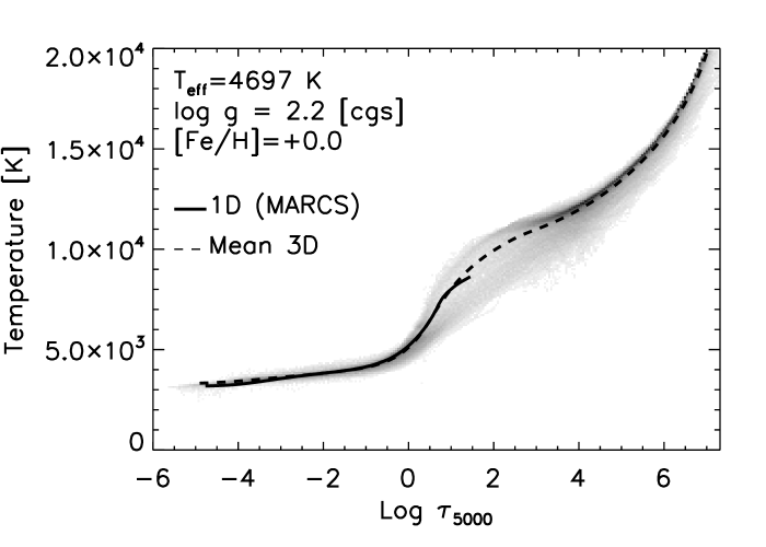
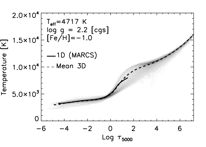
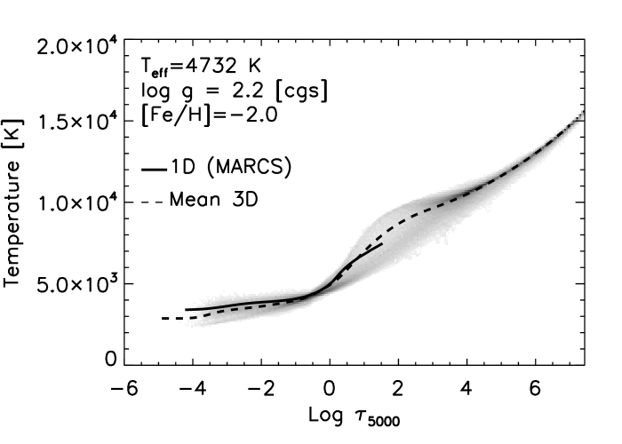
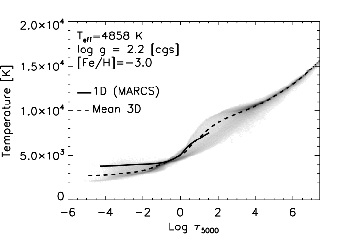
Figure 1 shows the temperature structures as a function of optical depth resulting from the convection simulations at K, compared with the 1D stratification from the corresponding marcs models. Figure 2 shows instead the temperature stratifications as a function of gas density for both the 3D simulations and 1D marcs model atmospheres. At solar metallicities and mild metal-deficiencies (), the mean temperature-density stratifications at a given optical depth in the upper atmospheric layers of the hydrodynamical simulations closely resemble the 1D structures of the corresponding marcs models where radiative equilibrium is enforced. At lower metallicities (), instead, the temperature stratification in the outer layers of the simulations tends to remain significantly lower than in 1D model atmospheres. The temperature in the optically thin layers of the convective simulations is for the most part regulated by two competing mechanisms: radiative heating caused by reabsorption by spectral lines of photons released at deeper layers, and adiabatic cooling following the expansion of the ascending gas. Following the interpretation given by Asplund et al. (1999) for 3D hydrodynamical models of metal-poor solar-type stars, with fewer and weaker lines available at low metallicities, adiabatic cooling becomes more dominant and the balance between cooling and heating occurs at lower surface temperatures than in radiative equilibrium conditions. At , the average temperature difference between 3D and 1D models in the upper atmospheric layers () is substantial and can amount to K or more at a given optical depth.
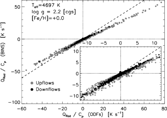
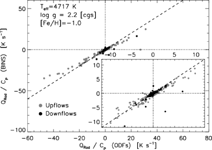
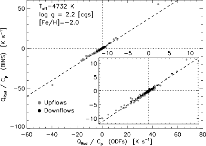
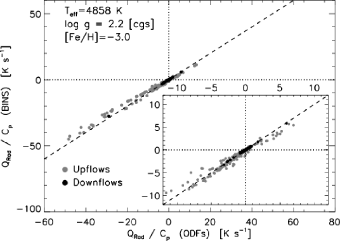
The prediction of photospheric temperatures significantly below radiative equilibrium values is a crucial result of the convection simulations. In order to test the accuracy of the opacity binning scheme in this respect, we computed the radiative heating rates in “1.5D” approximation for all columns in vertical slices of four red giant simulation snapshots with varying metallicities using the opacity binning approach and monochromatic radiative transfer with opacity distribution functions (ODFs). The results are compared in Fig. 3. At very low metallicities () there is an excellent correlation between the rates computed with the two approaches, suggesting that the opacity binning approximation is accurately reproducing the radiative heating and therefore also the temperatures at the surface of 3D metal-poor models. At solar metallicity and mild metal-deficiencies (), the correlation is somewhat poorer, and the results plotted in Fig. 3 show that the binning scheme generally leads to underestimate both the heating and the cooling rates compared with monochromatic radiative transfer using ODFs. Such weaker response to thermal fluctuations with the opacity binning approach corresponds to a looser coupling between matter and radiation which in turn increases the relative importance of convective cooling. This possibly implies that, at these metallicities, the opacity binning scheme is likely to slightly underestimate the temperatures in the upper photospheric layers.
Differences between the mean 3D and 1D atmospheric thermal structures, as well as the presence of temperature and density inhomogeneities in the 3D hydrodynamical simulations, can have dramatic effects on the predicted strengths of spectral lines. The cooler surface layers encountered in the convection simulations of metal-poor stars are expected to have a significant impact on temperature sensitive features, This is the case of, in particular, molecular lines and weak low-excitation lines of neutral metals, the line formation regions of which are shifted outwards in metal-poor hydrodynamical models because of the lower photospheric temperatures. Also, as a consequence of the cooler mean temperature stratifications, in the upper photospheric layers of metal-poor stars, the gas and electron pressure resulting from the convection simulations tend to remain lower than in the corresponding 1D hydrostatic models (see Asplund & García Pérez 2001). The lower gas and electron pressures in the metal-poor 3D hydrodynamical simulations are therefore expected to influence the formation of gravity sensitive lines.
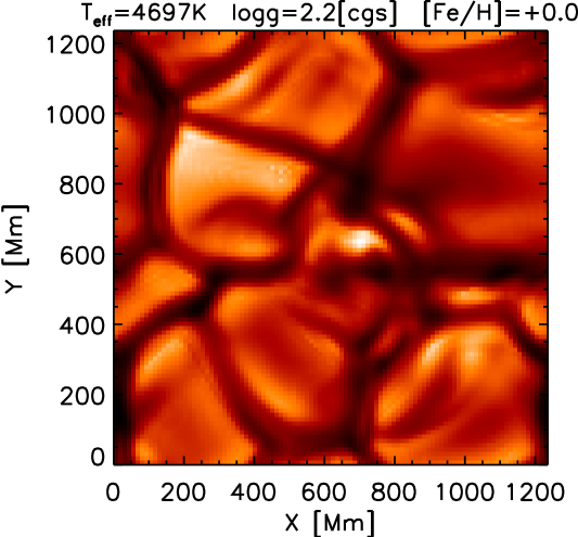
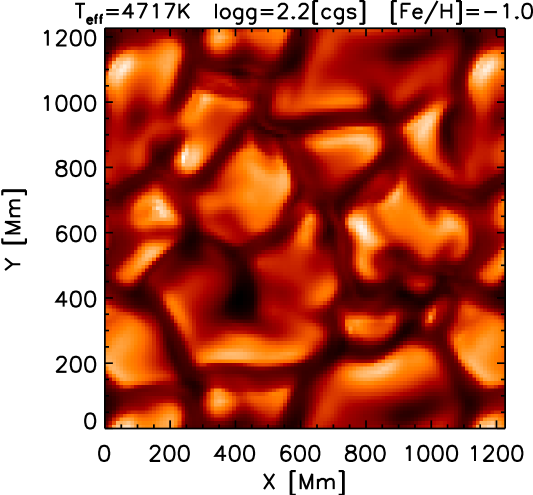
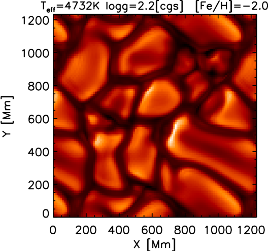
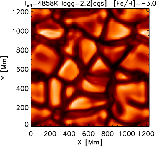
Figure 4 shows the spatially resolved outgoing intensity in the continuum bin for four snapshots of the simulations of the K series. The granulation pattern is clearly visible and qualitatively resembles the one observed on the Sun and in other simulations of late-type stars. The characteristic size of the granules varies depending on the metallicity of the simulations. The size of granules may be shown to scale approximately with the pressure scale height (e.g. Schwarzschild 1975). and with the ratio of horizontal to vertical flow velocities (Stein & Nordlund 1998). At low [Fe/H], the continuous opacity is lower and thus the gas density is higher at a given optical depth. This means that smaller vertical velocities are sufficient to sustain the convective flux. With smaller vertical velocities, horizontal velocities are also expected to be smaller. In practice, we observe that, in the proximity of the optical surface and below it (), the decrease in is overcompensated by a more pronounced decrease in , so that the product becomes in fact systematically larger the higher the metallicity of the simulation, suggesting that granules must also be bigger. We also find that the size of the granules increases with the effective temperature of the simulations. We intend to return to a more detailed description of the physical properties of the convection simulations in a future paper.
2.2 Spectral line formation
We use the red giant convection simulations as time-dependent 3D hydrodynamical model atmospheres to perform detailed spectral line formation calculations. We follow here the same procedure adopted in other recent investigations of the effects of surface convection and granulation on solar and stellar spectroscopy (Asplund et al. 1999, 2000a, 2000b, 2005; Asplund 2000; Asplund & García Pérez 2001; Allende Prieto et al. 2001, 2002b; Nissen et al. 2002; Collet et al. 2006). From the full red giant simulations, we select representative sequences, typically 100 to 250 hours long (stellar time), of about 30 snapshots separated at regular intervals in time. Prior to the line formation calculations, we decrease the horizontal resolution of the simulations from down to to ease the computational burden. We also interpolate the simulations to a finer depth-scale, increasing the vertical resolution of the layers with to improve the numerical accuracy.
We compute flux profiles for lines of a number of ions and molecules under the assumption of LTE. As the main purpose of our study is to isolate and investigate the impact of 3D models on LTE spectral line formation, we have not performed calculations on a large selection of lines ordinarily used in abundance analyses. Instead we consider a sample of “fictitious” atomic (Na i, Mg i, Ca i, Fe i, and Fe ii) and molecular (CH, NH, and OH) lines at selected wavelengths, with varying lower-level excitation potentials and line strengths (Steffen & Holweger 2002; Asplund 2005; Collet et al. 2006). Concerning molecular lines, we restrict our investigation to a set of low-excitation ( to eV) features representative of molecular bands frequently used in abundance analyses of giants (e.g. Christlieb et al. 2004; Bessell et al. 2004; Cayrel et al. 2004; Spite et al. 2005): CH lines at Å belonging to the AX electronic transition band, the OH AX system at Å, and the NH AX lines at Å. Fictitious lines provide a bench-mark for a systematic comparison of 1D and 3D LTE spectral line formation for various elements and molecules at different metallicities. They allow us to analyse the behaviour of spectral lines in 1D and 3D models uniquely as a function of lower-level excitation potential, wavelength and line strength, separating it from other complications such as blends or wavelength dependence of continuous opacities. Finally, in addition to the fictitious spectral lines, we also consider some real transitions of particular interest for stellar spectroscopy: the Li i line at Å and the forbidden [O i] lines at Å and Å.
When computing ionization and molecular equilibria and continuous opacities for the line formation calculations, we assume the same chemical compositions as used for the construction of the model atmospheres. As a rule, only the abundances of the trace elements are varied when calculating line opacities for the 3D cases. The number densities of line absorbers are then calculated from Saha ionization and Boltzmann excitation balances and instantaneous molecular equilibrium at the local temperature. Partition function data for atoms and ions are taken from Irwin (1981) and for molecules, together with equilibrium constants, from Sauval & Tatum (1984).
The source function for lines and continuum is approximated with the Planck function () and scattering is treated as true absorption. We discuss the validity of this approximation for the present analysis in Sect. 4.1. The radiative transfer equation is solved numerically along nine directions (two -angles, four -angles plus the vertical), after which we perform a disk integration and a time average over all selected snapshots. Various test calculations using a larger number of rays (four -angles, eight -angles plus the vertical) indicate that, for the scope of the present analysis, our procedure is accurate enough in reproducing the spatially and temporally averaged line profiles; the differences between elemental abundances determined with our procedure and the test cases are typically less than dex. In terms of derived abundances, temporal averaging over the selected number of snapshots is sufficient to obtain results with the same degree of accuracy, as verified by test calculations using different numbers of simulation snapshots.
To estimate the impact of 3D hydrodynamical models on stellar spectroscopy, we perform a differential abundance analysis using a simple curve-of-growth method. First, we calculate the LTE equivalent widths of the lines of our sample for a given chemical composition using 1D marcs models. We then evaluate the 3D1D LTE abundance corrections by varying the abundances in the 3D line formation calculations until the equivalent widths reproduce the ones computed in 1D. Spectral line profiles are calculated for typically 60 to 100 wavelength points depending on the strength of the lines. Test calculations performed increasing the spectral resolution of the line profiles ensure that the accuracy of the differential 3D1D analysis is consistently better than dex with the adopted number of wavelength points.
Particular care is exerted when dealing with OH and CH lines. The LTE number densities of the two hydrides in the upper photospheric layers show a highly non-linear dependence not only on temperature but also on the relative abundances of carbon and oxygen. Because of the relatively large dissociation energy of the CO molecule ( eV), the formation of carbon monoxide can significantly reduce the densities of both oxygen and carbon available for OH and CH. Therefore, in order to properly evaluate 3D1D effects for CH and OH lines, we are forced to take into account the simultaneous variation of carbon and oxygen abundances in the 3D line formation calculations. Here, we determine the 3D1D corrections to and abundances self-consistently, by means of an iterative procedure. The analysis of NH lines, on the contrary, is not affected by such complications: changes in and abundances have, in fact, altogether negligible effects on the strength of NH lines. This simplifies the task of determining of 3D1D corrections from these lines as variations of the abundance can be studied independently from the exact value of the and abundances. Vice versa, varying the abundance in the spectral line formation calculations causes no appreciable changes on the strengths of CH and OH lines.
The same numerical code and input physics are adopted for the line formation calculations with both 1D and 3D model atmospheres. In the 1D cases, we compute spectral line profiles for two different values of the micro-turbulence, km s-1 and km s-1, corresponding to the typical range of values adopted in ordinary 1D abundance analyses of red giants with similar stellar parameters as the ones adopted for our suites of models. We emphasize, however, that none of the fudge parameters needed in the classical 1D analyses (i.e. mixing length parameters, micro- and macro-turbulence) enters the 3D spectral line formation calculations: only the velocity fields inherent to the hydrodynamical simulations are here used to reproduce non-thermal line broadening and asymmetries associated with convective Doppler shifts.
For the fictitious lines we implement collisional broadening by hydrogen atoms according to the classical description by Unsöld (1955) with an enhancement factor of for the broadening constant. For the real features analysed here (Li i and [O i] lines) we apply instead the quantum mechanical calculations by Barklem et al. (2000).
As we limit our investigation to a differential analysis, we do not attempt to determine absolute 3D LTE abundances, but we rather address the question whether systematic effects are present in classical stellar spectroscopy based on 1D models. The main advantage of performing a differential study is that the sensitivity of the results to uncertainties in background continuous opacities, input physics, absolute line parameters (e.g. lower-level excitation potentials and values), collisional broadening, or blends can be minimized.

3 Results
3.1 Fe i and Fe ii lines
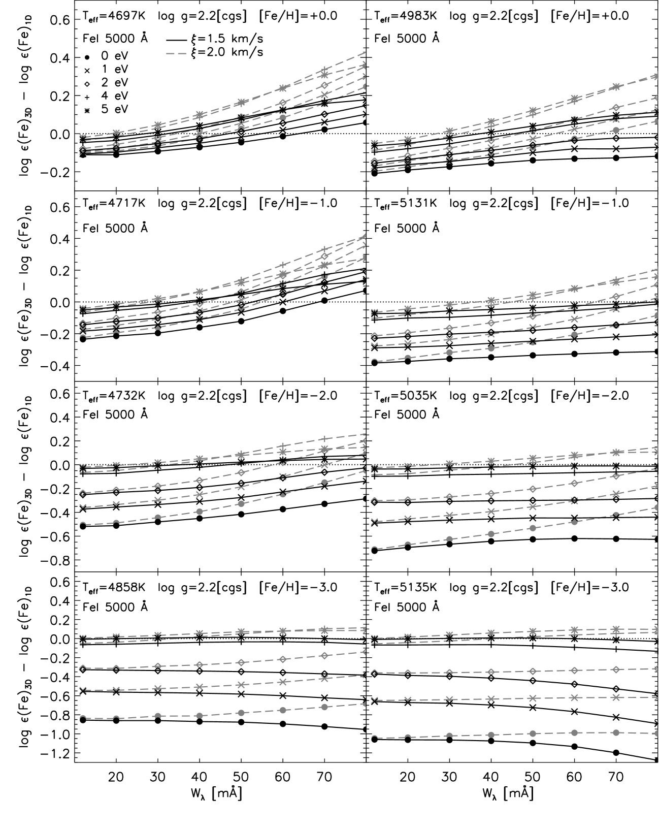
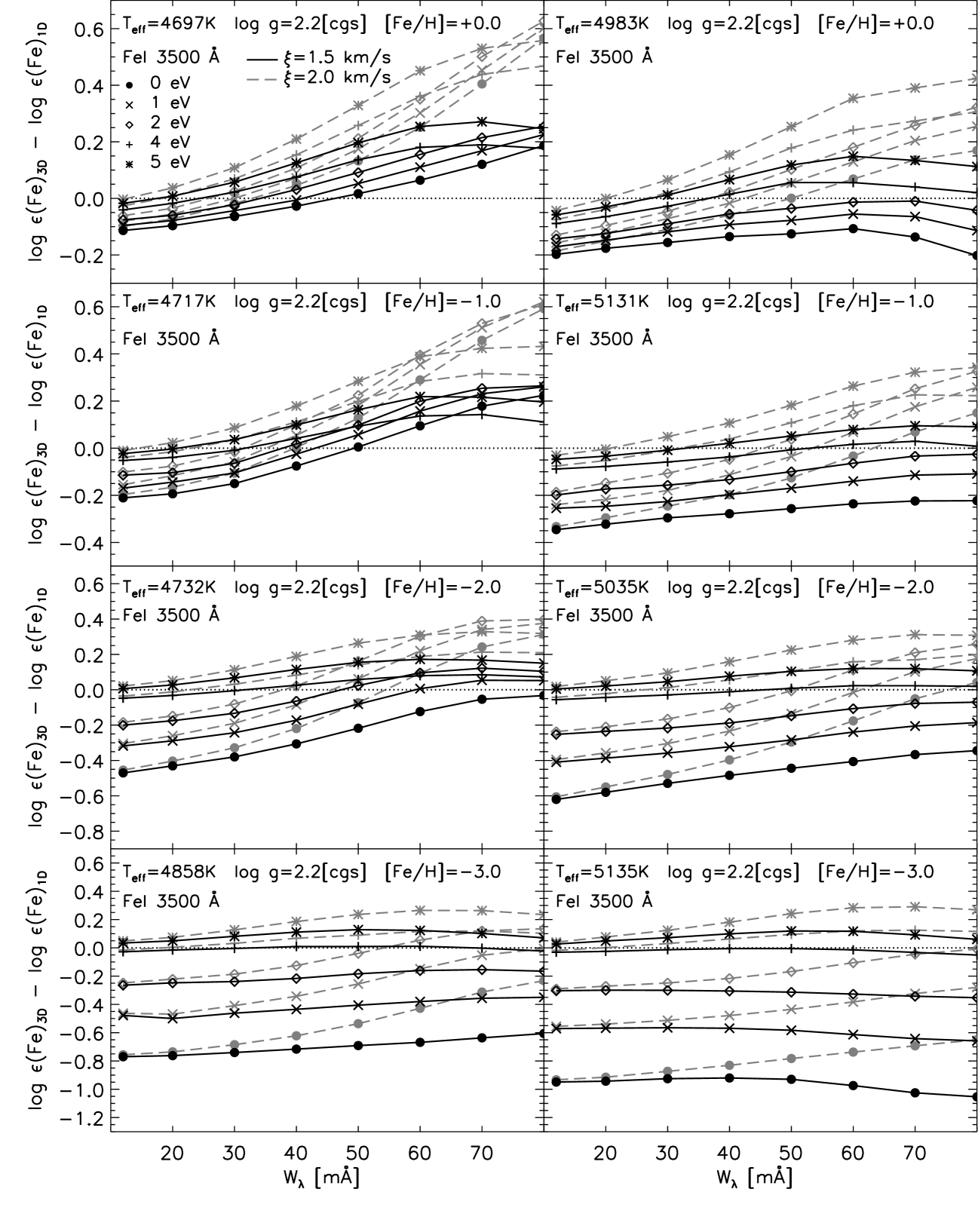
Figure 5 shows the 3D1D LTE corrections to the abundance as derived, for the two series of model atmospheres, from Fe i lines at Å with varying equivalent widths . At a given wavelength, the magnitudes of the corrections and their trends as a function of line strength depend on several parameters such as lower-level line excitation potential, metallicity, and effective temperature of the models.
At a given abundance, weak low-excitation Fe i lines appear stronger in the framework of 3D models than they do in 1D, resulting in negative 3D1D LTE abundance corrections. The effects are more pronounced at lower metallicities where the differences between the 3D and 1D abundances can reach dex. The 3D1D abundance corrections become progressively smaller for higher-excitation lines, vanishing for line excitation potentials of approximately eV. A similar result characterizing granulation abundance corrections for the Sun is reported by Steffen & Holweger (2002). In their spectroscopic analysis of the red giant Pollux ( Gem), Ruland et al. (1980) find that abundances derived for low-excitation lines are typically lower than for high-excitation lines and interpret the result as an effect of departures from LTE. Applying our 3D1D corrections, the trend of the derived abundances as a function of excitation potential would become even steeper, suggesting that the non-LTE effects might be even larger for the 3D case. Possible departures from LTE of are discussed further in Sect. 4.2
The overall behaviour of the 3D1D abundance corrections as a function line strength varies significantly depending on the metallicity of the models. At solar and moderately low metallicities (), the differences between 3D and 1D abundances become progressively less negative with increasing line strength and may eventually revert sign, growing positive for sufficiently strong lines and relatively high excitation potentials. It is also worthwhile observing that the abundance corrections for strong lines can reach a maximum and then turn-over as the line excitation potential increases. At lower metallicities, the 3D1D abundance corrections generally show a shallower trend with equivalent width. In particular, at , the corrections can also grow more negative for stronger lines. The values of the 3D1D abundance corrections for relatively strong lines ( mÅ) also depend on the choice of micro-turbulence, which controls the saturation level of the lines in the 1D calculations. At a given abundance in 1D the larger the micro-turbulence, the stronger the lines and in turn the less negative (or more positive) the differences between 3D and 1D abundances become.
Figure 6 shows analogous 3D1D abundance corrections computed for Fe i lines at Å. The results are fairly similar to the ones for Fe i lines at Å, the trends of the corrections following qualitatively the same behaviour as a function of line strength. The exact values of the corrections can vary slightly for the two wavelengths due to the different steepness of the source function with depth and different sensitivity of the continuous opacity at Å and Å to temperature and electron density.
In general, identifying the leading reason for a particular behaviour of the 3D1D corrections as a function of the line or the model parameters is not a simple task, due to the complexity and non-linearities inherent to line formation, in particular in 3D hydrodynamical models. In practice, spectral lines form over a relatively large range of optical depths; in the framework of 3D models line formation is sensitive not only to the mean thermal stratification but also to inhomogeneities in the temperature, density, and velocity fields. The large abundance corrections for weak lines in the very metal-poor cases can be qualitatively understood by comparing the 3D and 1D model structures. The mean temperature stratifications at the surface of 3D hydrodynamical simulations of very metal-poor giants are significantly cooler than in 1D models computed for the same stellar parameters (Sect. 2.1). This implies that in LTE the fraction of neutral to ionized iron is overall enhanced in the upper layers of 3D metal-poor models compared with the 1D case. The cooler temperature structure of 3D models also contributes to reducing the electron pressure and, consequently, lowering the density of - ions, thus decreasing the opacity in the continuum-forming layers. Therefore, at low metallicities, the combined effect of increased line opacity and decreased continuous opacities tends to make weak low-excitation Fe i lines stronger in 3D than in 1D; a lower abundance is then required in metal-poor 3D models to reproduce the 1D equivalent widths.
Weak high-excitation lines form in deeper photospheric layers and are less sensitive to the temperature structure at the surface of the models. At all metallicities, the resultant 3D1D abundance corrections for high-excitation lines are smaller than for the low-excitation features. Stronger lines form higher up in the atmosphere compared with weak lines when the other line properties remain the same. While at very low metallicities Fe ii is clearly the dominant ionization stage nearly everywhere in the 1D models, in 3D the Fe i fraction is substantial at all depths contributing to the emergent line profiles. Therefore in very metal-poor models the 3D1D abundance corrections typically remain negative for strong Fe i lines. As a test, we compute curves-of-growth of Fe i lines using the horizontally averaged 3D structure to quantitatively study the dependence of line strengths on the lower temperatures of the mean stratification. The behaviour of the 3D1D corrections for Fe i lines can be qualitatively reproduced by comparing the curves-of-growth for the 1D marcs and mean 3D stratifications. The test confirms that the lower temperatures encountered in the 3D hydrodynamical metal-poor model atmospheres are the main factor determining the large and negative 3D1D corrections. However, we emphasize that, from a quantitative point of view, line formation calculations relying on the mean 3D stratification cannot accurately reproduce the results of the calculations based on the actual 3D model atmospheres. In fact, abundances derived from weak low excitation Fe i lines using the full 3D and the mean 3D stratifications can differ by up to about dex. This is an indication that the temperature and velocity inhomogeneities of the 3D structure should not be neglected.
At metallicities closer to solar, the trends of 3D1D abundance corrections with line strength cannot be ascribed simply to differences between 1D and mean 3D stratifications, which are very similar in the line forming layers. Curves-of-growth computed for Fe i lines using either the 1D marcs models or the mean 3D stratifications (and the same value of micro-turbulence) closely resemble each other. The differences in abundance determinations using the 1D and mean 3D stratifications amount in fact to less than dex for Fe i lines within the range of line strengths considered here. Hence, the actual trends of the 3D1D corrections at metallicities near solar must be attributed mainly to 3D temperature inhomogeneities and possibly velocity fields. We also note that the trend of the 3D1D abundance corrections, increasing with equivalent width for , can be flattened by appropriately choosing a smaller value for the micro-turbulence than the ones considered here ( km s-1). However, typical micro-turbulences derived from spectroscopic 1D analyses of red giants are found indeed to be in the range between km s-1 and km s-1. At metallicities , the present 3D1D abundance corrections, would therefore introduce a trend in the derived abundances as a function of equivalent width. This could be an indication that convective motions of the gas are not fully resolved in the present hydrodynamical simulations and, consequently, that non-thermal Doppler broadening is also underestimated. Further investigation is however necessary in order to identify other possible causes for these trends.
We observe that the 3D1D abundance corrections for lines at a given equivalent width are typically shifted toward more negative values for the higher effective temperature models. The equivalent width of a (weak) spectral line is roughly proportional to the ratio of line to continuous opacity at line formation depth (see also Gray 1992, p. 277). In the case of (weak) low-excitation Fe i lines, for a given abundance, the ratio turns out to be larger the higher the effective temperature of the models at all metallicities, indicating that 3D1D abundance corrections are also expected to be more pronounced (more negative).
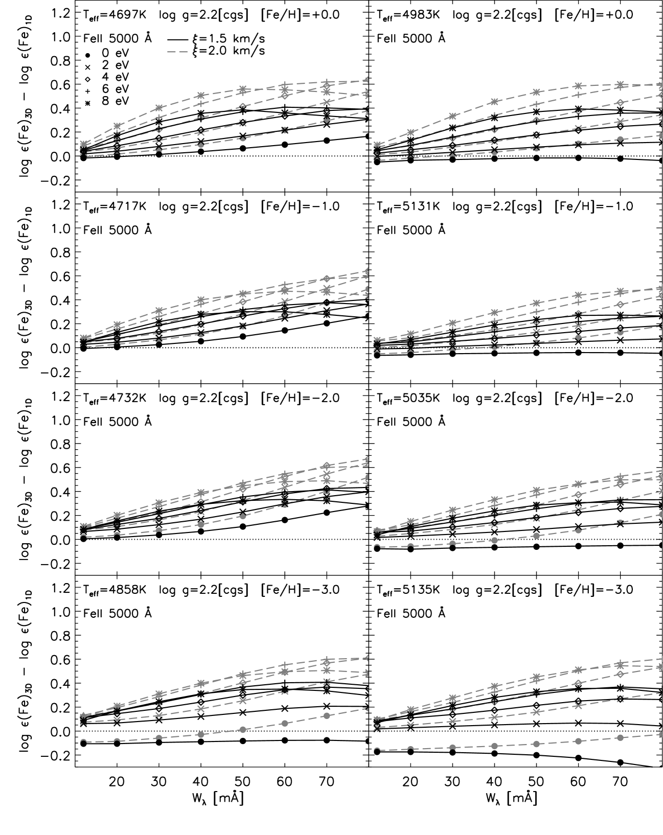
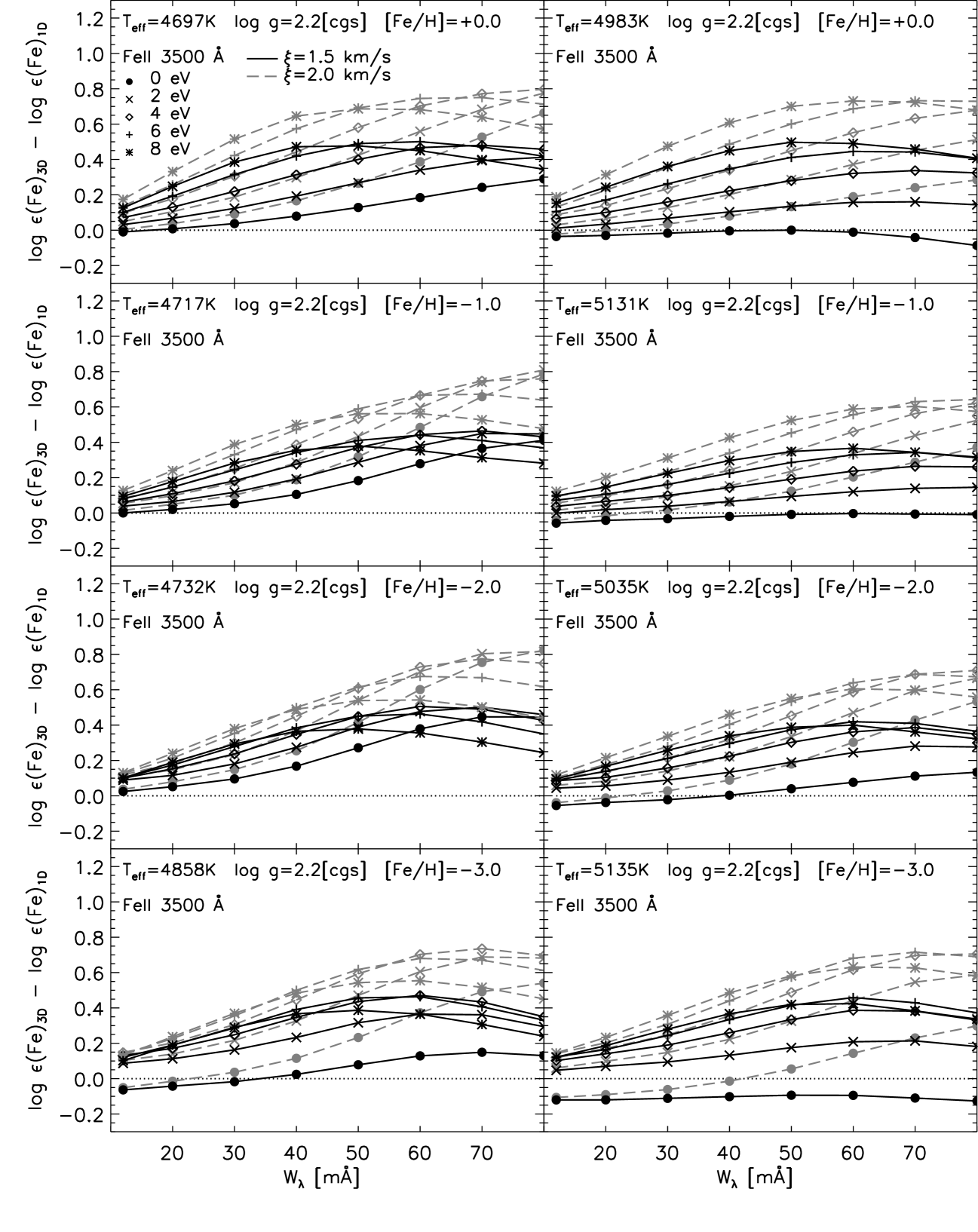
The 3D1D abundance corrections for Fe ii lines at Å and Å are presented in Fig. 7 and 8. The overall trends of the corrections for these lines are similar at all metallicities; differences between abundances derived with 3D and 1D models are typically positive and generally increase with increasing line strength and excitation potential. Low-excitation lines can, however, show negative corrections at metallicities below . Similarly as for Fe i lines also, the corrections Fe ii lines at a given equivalent width can reach a maximum and revert their trend for sufficiently high excitation potentials. This behaviour is also present in 3D1D abundance corrections for lines of neutral and ionized metals in solar-type stars (Asplund 2005), although evident already for somewhat weaker lines.
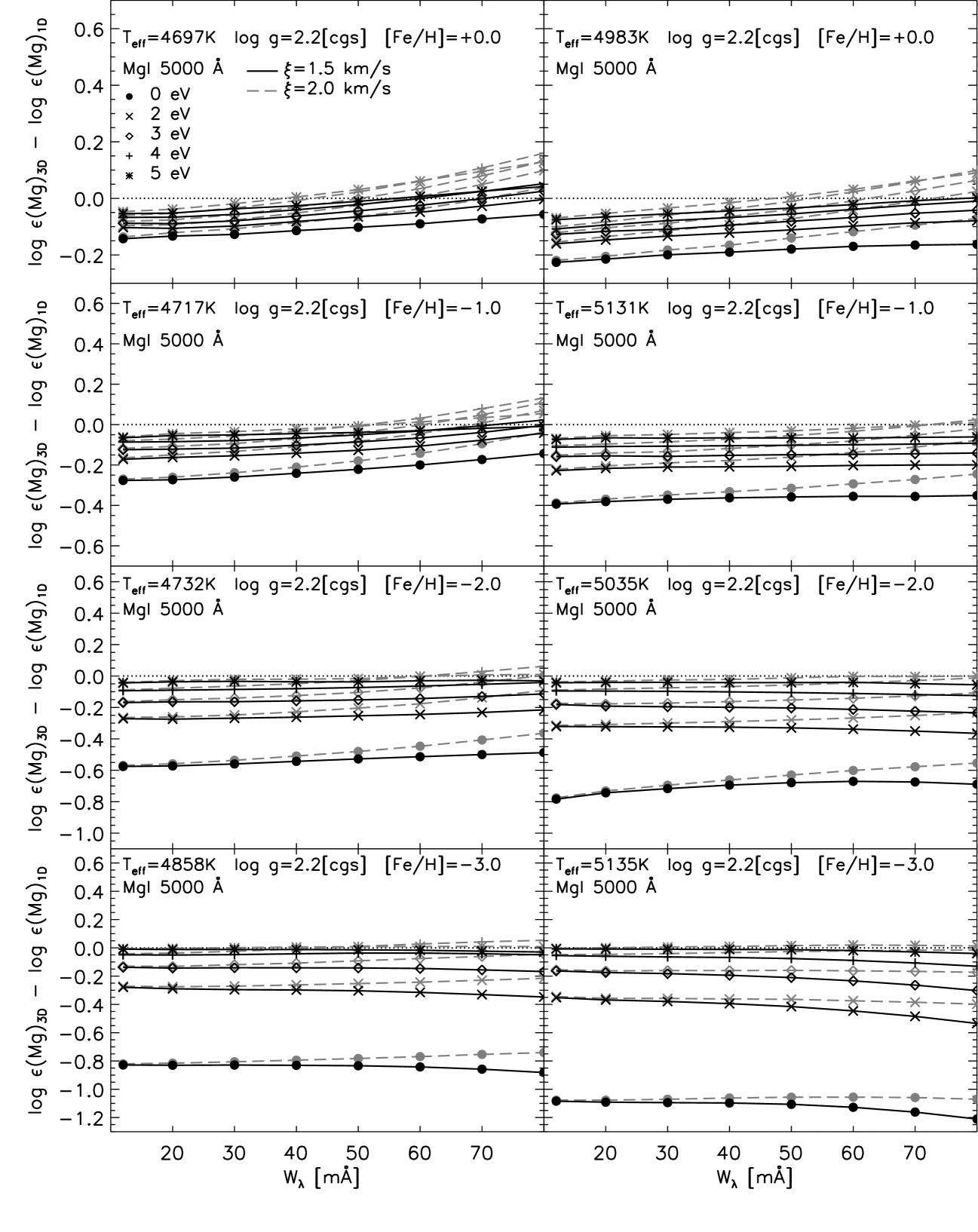
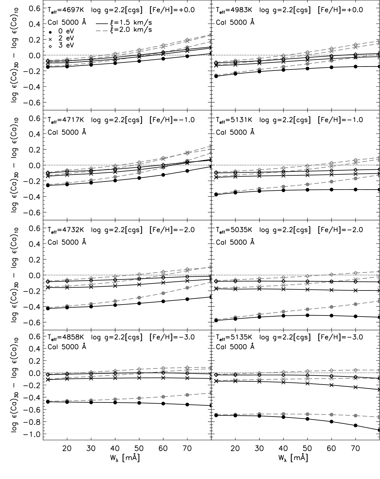
3.2 Na i, Mg i, and Ca i
Figures 9, 10, and 11 show the 3D1D LTE corrections to the sodium, magnesium, and calcium abundances as derived from Na i, Mg i, and Ca i lines at Å. The behaviour of the abundance corrections as a function of line strength for these lines is similar to the one predicted for Fe i lines. In LTE, the overall trends of the corrections are governed by the differences between the 1D and mean 3D temperature stratifications and by the presence of temperature inhomogeneities and velocity fields in the 3D models. The actual magnitude of the 3D1D effects, however, largely depends on the ionization potential of the species under consideration. The 3D1D abundance corrections for Na i and Ca i, for instance, are considerably smaller than the ones derived from Fe i lines. In fact, the relatively low ionization potentials of Na i and Ca i imply that the two metals are more easily ionized compared with Fe i, both in 1D and 3D models. This significantly reduces the 3D1D effects on line strengths due to temperature inhomogeneities or differences in the thermal stratifications. Magnesium on the contrary has a fairly high first ionization potential, comparable to that of iron: hence, the computed 3D1D abundance corrections for Mg i lines are typically also as large as the ones derived from Fe i lines.
3.3 Li i
| 1.0 | 0.90 | 37.7 | ||||
| 1.0 | 0.77 | 34.7 | ||||
| 1.0 | 0.62 | 30.1 | ||||
| 1.0 | 0.55 | 22.0 | ||||
| 1.0 | 0.78 | 17.5 | ||||
| 1.0 | 0.66 | 11.7 | ||||
| 1.0 | 0.56 | 14.7 | ||||
| 1.0 | 0.50 | 12.7 |
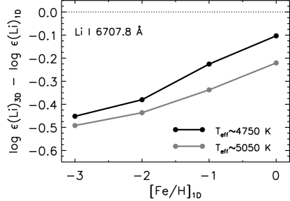
Lithium abundances in stars are of great importance in astrophysics: they can be used as diagnostics of stellar evolution, primordial nucleosynthesis as well as cosmic and Galactic chemical evolution. Nearly all stellar abundance determinations in late-type stars are based on the analysis of the Li i resonance line at Å. In order to accurately determine abundances it is therefore necessary to properly model the formation of this line, taking into account possible effects due to stellar granulation as well as departures from LTE in general. Recent investigations of 3D/1.5D non-LTE Li i spectral line formation in the Sun (Kiselman 1997, 1998; Uitenbroek 1998) and metal-poor solar-type stars (Asplund et al. 2003; Barklem et al. 2003) indicate that non-LTE effects on the derived abundances are significant and comparable to the ones due to granulation. In the present study, however, we only explore the effects of granulation on the formation of the Li i Å line under the approximation of LTE; a detailed 3D non-LTE analysis of Li i line formation in giant stars is deferred to a future paper. In Table 2 (Fig. 12), we present the 3D1D LTE corrections to abundances derived from the Li i Å line, assuming a value of at all metallicities in the 1D calculations. The overall 3D1D LTE abundance corrections as a function of metallicity behave rather similarly to the ones derived for weak ( mÅ) low-excitation lines of other neutral elements. Since, the ionization potential of Li i is just slightly larger than the one of Na i, the 3D1D LTE corrections for these two species are typically very similar.
Once again, the differences between the 3D and 1D abundances are relatively large and negative ( dex) at very low metallicities, because of the markedly cooler temperature structures of 3D model atmospheres compared with the 1D cases, while they become gradually smaller as metallicity increases. Also, as for neutral lines in general, 3D1D LTE abundance corrections are more pronounced for the series of model atmospheres with higher .
3.4 [O i] lines
| Å | Å | ||||
| 8.89 | 8.90 | 8.88 | |||
| 7.89 | 7.87 | 7.86 | |||
| 6.89 | 6.87 | 6.87 | |||
| 5.89 | 5.77a | 5.77a | |||
| 8.89 | 8.89 | 8.87 | |||
| 7.89 | 7.83 | 7.83 | |||
| 6.89 | 6.81 | 6.81 | |||
| 5.89 | 5.71a | 5.71a | |||
| 8.39 | 8.36 | 8.35 | |||
| 7.39 | 7.33 | 7.33 | |||
| 6.39 | 6.23 | 6.23a | |||
| 8.39 | 8.33 | 8.32 | |||
| 7.39 | 7.28 | 7.28 | |||
| 6.39 | 6.17 | 6.17a |
-
a
The equivalent width of the line is less than mÅ.
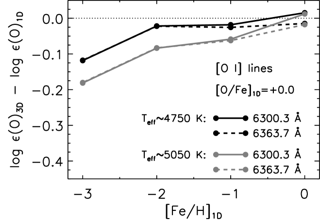
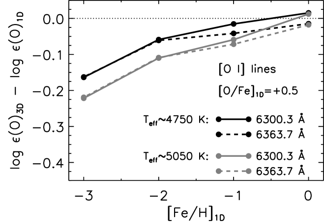
The [O i] forbidden lines at Å and Å are among the most widely used indicators of abundance in cool stars and halo giants ( K) in particular (e.g. Barbuy 1988; Allende Prieto et al. 2001; Nissen et al. 2002; Spite et al. 2005; García Pérez et al. 2006) The main advantage concerning the use of [O i] lines is that they are expected to form under LTE conditions (Kiselman 2001); the drawback is, on the other hand, that these lines tend to become, in general, very weak already at in stars with similar surface gravities as the ones considered here.333At and with , the equivalent widths of the two [O i] lines at Å and Å computed using the marcs model atmosphere at K are mÅ and mÅ, respectively. The existence of oxygen over-abundances with respect to iron in metal-poor stars has been pointed out already by Conti et al. (1967). The exact amount of the over-abundances, however, and their overall trend with metallicity is still today a matter of debate (García Pérez et al. 2006). In our analysis, we therefore consider, for simplicity, two different values of oxygen enhancement with respect to the scaled solar standard compositions for the 1D spectral line formation calculations: and (for ).
In Table 3, we present the differential 3D and 1D abundances as derived from the two [O i] lines. The trends of the 3D1D abundance corrections as a function of metallicity or effective temperature of the models (Fig. 13) are qualitatively the same as in the case of the other neutral species discussed above. Nonetheless, the 3D1D corrections for [O i] forbidden lines are in general significantly smaller. Because of its high ionization potential ( eV), O i is, in fact, the dominant ionization stage for oxygen in the line formation layers of both 3D and 1D models and shows rather little sensitivity to the differences between the 3D hydrodynamical and 1D hydrostatic temperature stratifications at the surface (see also Sect. 3.2). The small differences between the two [O i] lines in terms of abundance corrections are due to the different formation depths of the two features.
| eV | eV | eV | eV | |||||||
| 8.89 | 8.52 | 8.80 | 8.80 | 8.44 | 8.45 | |||||
| 7.89 | 7.52 | 7.71 | 7.73 | 7.43 | 7.44 | |||||
| 6.89 | 6.52 | 6.61 | 6.66 | 6.42 | 6.44 | |||||
| 5.89 | 5.52 | 5.08 | 5.19 | 4.94 | 5.04 | |||||
| 8.89 | 8.52 | 8.71 | 8.73 | 8.37 | 8.39 | |||||
| 7.89 | 7.52 | 7.62 | 7.66 | 7.33 | 7.35 | |||||
| 6.89 | 6.52 | 6.37 | 6.47 | 6.22 | 6.26 | |||||
| 5.89 | 5.52 | 4.76 | 4.93 | 4.65 | 4.79 | |||||
| 8.39 | 7.52 | 8.21 | 8.23 | 7.44 | 7.45 | |||||
| 7.39 | 6.52 | 7.06 | 7.11 | 6.45 | 6.46 | |||||
| 6.39 | 5.52 | 5.49 | 5.63 | 5.03 | 5.12 | |||||
| 8.39 | 7.52 | 8.14 | 8.18 | 7.37 | 7.38 | |||||
| 7.39 | 6.52 | 6.88 | 6.96 | 6.27 | 6.33 | |||||
| 6.39 | 5.52 | 5.14 | 5.35 | 4.74 | 4.88 |
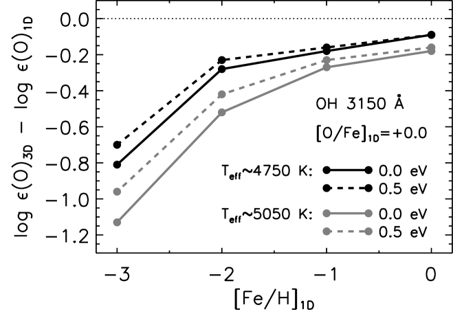
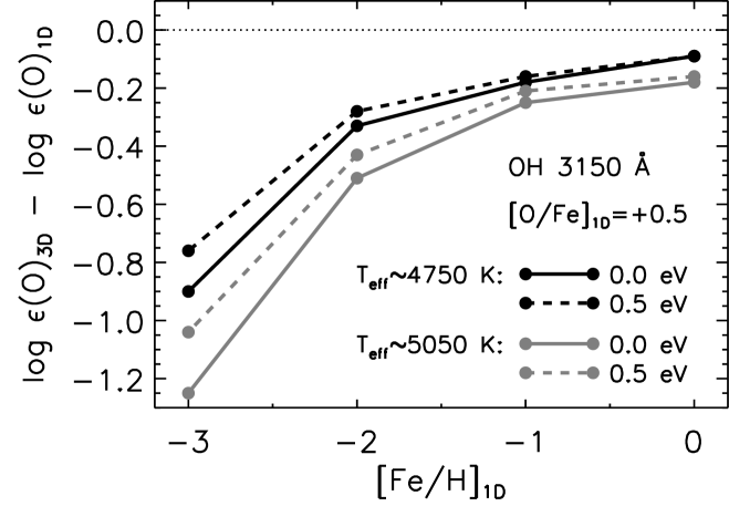
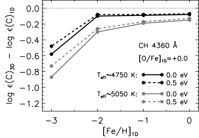
3.5 CH, NH, and OH lines
Molecule formation shows an extreme and highly non-linear sensitivity to temperature in the upper layers of late-type stellar photospheres. Because of this strong temperature dependence, molecular lines are very susceptible to systematic errors in the thermal structure of the model atmospheres. In 3D model atmospheres, the vertical temperature gradients are typically steeper in upflows than in downdrafts. The temperature contrast reverses in the upper photosphere some distance above the optical surface, so that the gas above the granules becomes cooler than average in the overshoot region (Stein & Nordlund 1998). The temperature contrast in these layers is more pronounced for the lower metallicity models where the coupling between the radiation field and the gas is weaker. Temperatures in the high photospheric layers are generally low; however, compression due to converging gas flows or shocks at the boundaries between granules heat the fluid in the intergranular lanes, raising the temperature above the radiative equilibrium value. Consequently, the strengths of molecular lines are expected to vary across the surface of the model atmospheres, being stronger in the upflowing regions. Also, the formation of the spatially and temporally resolved molecular line profiles is biased towards granules because of their large area coverage, steeper temperature gradients, and higher continuum intensities.
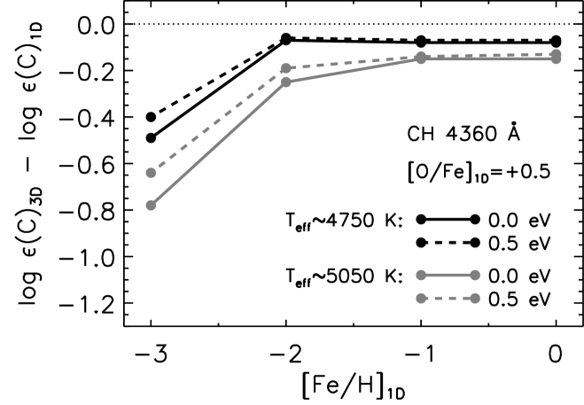
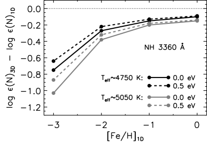
The significantly lower temperatures of the upper photospheric regions of 3D metal-poor model atmospheres compared with their 1D counterparts favour higher concentrations of CH, NH, and OH molecules for a given chemical composition, therefore resulting in stronger molecular lines and negative 3D1D C, N, and O abundance corrections. Differences between the 3D and 1D predicted molecular line strengths are less pronounced at higher metallicities, in accordance with the similarities between the 1D and mean 3D temperature stratifications, and are ascribable primarily to the temperature inhomogeneities in the 3D structures.
In Tables 4 and 5 we present the 3D1D LTE C, N, and O abundance corrections derived from weak fictitious CH, NH, and OH lines (with equivalent widths mÅ), as a function of metallicity (see also Fig. 14 and 15). At very low metallicities (), the 3D1D corrections are very large and negative and range between and dex for the cases here considered. As expected, the differences between 3D and 1D abundances become gradually less pronounced at higher metallicities, reducing to values of approximately dex at . The actual magnitude of the abundance corrections for molecular features depends on several factors such as the species under consideration, the line parameters (in particular the lower level excitation potential), and the effective temperatures of the models. The 3D1D effects for higher excitation lines at a given metallicity are generally smaller in accordance with the sensitivity of these lines to deeper layers where the temperature differences between 3D and 1D models are less prominent. The overall larger corrections for hotter models are in agreement with the larger 3D1D temperature differences in very metal-poor stars and, at near solar metallicities, with the presence of temperature inhomogeneities in the 3D structure and the high non-linearity of molecule formation.
The magnitudes of the corrections for CH, NH, and OH lines naturally depend on the details of the molecular equilibrium with other species, and the various indicators in practice show different sensitivities not only to the photospheric temperature structure but also to the chemical composition. For instance, at very low metallicities, the corrections for NH and CH lines differ by up to dex in spite of the similar dissociation energies of the two molecules ( eV and eV, respectively). Line strengths of CH and OH molecules are also sensitive to both carbon and oxygen atomic abundances. In Table 4 (Fig. 14) we compare the results of 3D1D analyses on OH and CH lines performed assuming, for the 1D calculations, two different values of oxygen enhancement with respect to the scaled solar standard compositions: and (for ), with all other metals regularly scaled as usual by the same amount as iron. Changes in the oxygen abundance alter the number densities of of both OH and CH molecules by different amounts in 3D and 1D. In particular, increasing from to in the 1D calculations results in overall larger 3D1D abundance corrections for OH lines and smaller corrections for CH lines. In practice, however, the effects on the abundance corrections are appreciable only at very low metallicities. The trends of 3D1D C and O abundance corrections from CH and OH molecular lines at low metallicity depend on the particular choice made here for the 1D chemical compositions (with ) and on the sensitivity of molecule formation to temperature in the coolest layers of 3D models. In the very metal-poor 1D giant models, most of the carbon and oxygen are in atomic form, due to the low surface gravity, the overall low C and O abundances, and the relatively high temperatures of the upper photospheric layers ( K or more). The fraction of carbon and oxygen atoms locked in CO molecules is negligible and increases only slightly when is changed from to . As a result, the 1D photospheric number density of CH molecules also remains approximately the same in both the and cases. On the contrary, in very metal-poor 3D models, temperatures can be significantly lower in the upper photosphere and, below K, a considerable fraction of carbon ends up locked in CO. As increases from to , the number density of CO in these cool layers increases further, reducing the amount of carbon available for the formation of CH molecules. Thus, while the number density of CH molecules is still larger than in 1D, the 3D1D C abundance corrections become smaller (less negative) if increases. In the case of oxygen, in the very metal-poor 1D models where the fraction of CO is negligible, the number density of OH molecules in the photosphere simply scales proportionally to the O abundance, i.e. it increases by a factor of when is raised from to . In the coolest layers of 3D models, where most of the carbon is locked in CO, the amount of oxygen available for OH molecule formation is also reduced. Assuming and that most carbon is in form of CO molecules, the amount of oxygen available to form OH molecules or remain in atomic form increases by a factor as high as as is changed from to ; that also explains why the 3D1D O abundance corrections derived from [O i] and OH lines become more pronounced as increases.
| eV | eV | ||||
|---|---|---|---|---|---|
| 8.01 | 7.91 | 7.92 | |||
| 7.01 | 6.86 | 6.88 | |||
| 6.01 | 5.74 | 5.79 | |||
| 5.01 | 4.26 | 4.37 | |||
| 8.01 | 7.86 | 7.87 | |||
| 7.01 | 6.81 | 6.83 | |||
| 6.01 | 5.63 | 5.69 | |||
| 5.01 | 3.98 | 4.14 |
4 Restrictions of line formation calculations
4.1 Scattering
The results of our analysis indicate that the differences between abundances derived from 3D and 1D model atmospheres of red giant stars can be considerable, especially at very low metallicities. The presence of large 3D1D corrections can have strong implications for the interpretation of stellar abundances in terms of Galactic chemical evolution. The current 3D analysis, however, still relies on a number of approximations and assumptions, which can possibly lead to systematic errors in the derived abundances and must therefore be discussed.
As mentioned in Sect. 2.1 and 2.2, we treat scattering as true absorption when solving the radiative transfer equation, both for the convection simulations and the line formation calculations with 3D and 1D model atmospheres. This assumption can in general lead to systematic errors in the predicted temperature stratification of the upper layers of 3D hydrodynamical model atmospheres where the contribution of scattering to extinction is significant, and, ultimately, affect the strengths of synthetic spectral lines. Rayleigh scattering of H i can contribute significantly to the total continuous extinction in the UV and blue part of the spectrum. At these wavelengths, implementing scattering as true absorption in the detailed line formation calculations underestimates, in general, the emergent flux in the continuum, resulting in too weak spectral lines (Cayrel et al. 2004). The effect is expected to be more pronounced in very metal-poor stars, where line-blocking in the continuum is weak, and, in particular, in metal-poor 3D model atmospheres, where the lower surface temperatures result in lower electron number densities and higher densities of scatterers (H i particles) relative to absorbers (namely - particles in the case of continuous absorption).
In order to quantify the effect of our approximated treatment of scattering on the photospheric stratifications, we have computed a series of 1D marcs model atmospheres of giant stars at various metallicities, including scattering as true absorption in the solution of the radiative transfer equation. The results of our test indicate that treating scattering as true absorption leads to hotter temperature stratifications compared with models in which scattering is properly taken into account (see also Gustafsson et al. 1975). Temperature differences at optical depth can reach K for model stellar atmospheres of very metal-poor red giants at ; for model atmospheres, the temperature differences at the same optical depth are smaller and amount to about K. On the sole basis of these results, one could be tempted to conclude that the temperatures at the surface of the metal-poor 3D hydrodynamical models might be over-estimated. However, further testing is needed to estimate the magnitude of the effect on the 3D temperature stratification in metal-poor stars, and, more importantly, to also assess whether, in this case, it proceeds in the same direction. Either way, the treatment of scattering as true absorption is likely to significantly affect the balance between radiative heating and adiabatic cooling in the upper photospheric layers.
We have also performed some test line formation calculations with the average 3D stratifications of our very metal-poor model red giant stellar atmospheres and using the the spectrum synthesis code bsyn from the Uppsala package, which treats continuum scattering properly within the LTE approximation. We find that including scattering as true absorption in the calculations has relatively little influence on the predicted line strengths, at least for the type of giants considered in our study. Nonetheless, the effect of the above assumption might, in practice, be larger in full 3D line formation calculations because of the presence of temperature and density inhomogeneities. The use of a differential 3D1D abundance analysis ensures, however, that the uncertainties in the treatment of scattering in the spectral line formation calculations are at least reduced.
4.2 Departures from LTE
It is important to emphasize that, in general, spectral lines of many of the species considered in our analysis are expected to suffer from departures from LTE. In particular, Fe i lines are most certainly seriously affected by non-LTE effects. The main non-LTE mechanism for in late-type stellar atmospheres is over-ionization, which is driven by the radiation field in the UV being larger than the Planck function at the local temperature . This causes efficient photo-ionization from Fe i, leading to underpopulation of all Fe i levels compared with LTE and to weaker Fe i lines. This, in turn, implies that abundances derived from Fe i lines are generally larger in non-LTE than with the assumption of LTE. At present, there is no consensus on how severe the non-LTE effects actually are on Fe i lines in late-type stars (see, e.g., discussion in Asplund 2005). Collet et al. (2006) have estimated the non-LTE effects on Fe i lines for the extremely metal-poor giant HE 01075240 by means of a 1D analysis based both on a marcs model atmosphere and the mean atmospheric stratifications inferred from 3D simulations. The non-LTE effects there are found to be considerable and opposite to the 3D1D LTE corrections, confirming that a combined treatment of both 3D and non-LTE effects is necessary for accurate abundance determinations. A full 3D non-LTE study of Fe i spectral line formation is certainly of high priority, but goes beyond the scope of the present work and is postponed to a future paper.
Similarly, lines of other species considered in this study, such as Li i, Na i, Ca i, and Mg i might form out of LTE conditions. Molecular lines might as well suffer from departures from LTE; however, non-LTE effects on molecular line formation are, still today, largely unexplored even in 1D analyses (Asplund & García Pérez 2001). In addition, molecule formation could also occur out of LTE: the rapid cooling occurring at the surface of the 3D simulations could imply that molecular equilibrium is not reached; also, photo-dissociations feeding on the radiation field coming from deeper layers might move the molecular equilibrium out of LTE. These aspects are undoubtedly worthy further investigation.
4.3 Stellar parameters
The derivation of accurate abundances requires not only realistic modelling of the structure of stellar atmospheres and of the processes of spectral line formation, but also appropriate determination of the fundamental stellar parameters. In the differential 3D1D analysis presented here, we have assumed the stellar parameters to be the same for both 3D and 1D model atmospheres. However, one could expect the determination of the stellar parameters for a given star to depend on whether 1D or 3D models are used (see also discussion in Asplund & García Pérez 2001). For instance, the results of our differential analysis of lines suggest that differences in the derived metallicities cannot indeed be excluded. Also, differences between the thermal structures of 3D and 1D model atmospheres can affect ionization equilibria and, therefore, the determination of spectroscopic surface gravities. Finally, temperature inhomogeneities in the continuum-forming layers of 3D hydrodynamical model atmospheres can, in general, lead to different emergent flux distributions compared with the predictions of 1D models and, consequently, affect effective temperature estimates.
The above discussion on the possible sources of systematic errors in the 3D modelling of stellar atmospheres and line formation can create the impression that the results presented here are rather uncertain and that analyses based on 1D model atmospheres are still preferable. It is important, however, to emphasize that many of the uncertainties in the present 3D analysis (e.g. departures from non-LTE and molecular equilibrium) apply as well to the 1D analysis, besides the systematic errors introduced, in the latter case, by the assumption of hydrostatic equilibrium and the rudimentary treatment of convective energy transport.
5 Conclusions
In the present work, we have investigated the impact of 3D hydrodynamical model atmospheres of red giant stars on the formation of spectral lines of various ions and molecules and on the derivation of elemental abundances. The differences between the mean 3D temperature stratifications and corresponding 1D model atmospheres as well as the presence of temperature and density inhomogeneities and correlated velocity fields in the 3D structure, can significantly affect the predicted line strengths and, hence, the values of elemental abundances derived from spectral lines. Differences between abundance determinations based on 3D and 1D models are particularly large at low metallicities. The temperatures in the upper layers of 3D hydrodynamical model atmospheres of metal-poor giant stars are in fact significantly lower than the ones predicted by classical 1D models computed for the same stellar parameters. Because of the cooler temperature stratifications of 3D model atmospheres, weak lines of neutral species and molecules appear considerably stronger in 3D than in 1D, under the assumption of LTE. The 3D1D corrections for these lines are large and negative. In particular, we find the 3D1D LTE corrections to CNO abundances derived from CH, NH, and OH weak low-excitation to be typically in the range dex to dex for the very metal-poor giants at considered here. We also derive large negative corrections to the abundances (about dex) at these metallicities, based on the analysis of weak low-excitation Fe i lines.
In Sect. 4, we finally discuss possible systematic errors affecting the present 3D abundance analyses. A major source of uncertainty in this respect is the approximated treatment of scattering as true absorption, both in the 3D convection simulations and in the line formation calculations. As discussed in Sect. 4.1, this approximation can lead to systematic errors in the estimated temperatures of the upper layers of 3D model atmospheres as well as in the predicted emitted fluxes in the UV, therefore the strengths of spectral lines. Also, the assumption of LTE is in general questionable for many of the ions and molecules considered in the analysis. In particular, in the case of iron, strong over-ionization feeding on the UV radiation field can lead to significantly weaker Fe i lines in metal-poor red giants stars compared with the cases where LTE is enforced. The effects of over-ionization on the strengths of Fe I lines are opposite to the ones of granulation. Departures from LTE should, therefore, accounted for in the 3D line formation calculations in order to accurately determine 3D1D corrections to the Fe abundances.
Acknowledgements.
The authors acknowledge support from the Swedish Foundation for International Cooperation in Research and Higher Education and the Australian Research Council. K. Eriksson and B. Gustafsson are thanked for fruitful discussions. Finally, the authors would like to thank the anonymous referee for the very positive and constructive criticism which helped improve the manuscript.References
- Allende Prieto et al. (2002a) Allende Prieto, C., Asplund, M., López, R. J. G., & Lambert, D. L. 2002a, ApJ, 567, 544
- Allende Prieto et al. (2001) Allende Prieto, C., Lambert, D. L., & Asplund, M. 2001, ApJ, 556, L63
- Allende Prieto et al. (2002b) Allende Prieto, C., Lambert, D. L., & Asplund, M. 2002b, ApJ, 573, L137
- Asplund (2000) Asplund, M. 2000, A&A, 359, 755
- Asplund (2005) Asplund, M. 2005, ARA&A, 43, 481
- Asplund et al. (2003) Asplund, M., Carlsson, M., & Botnen, A. V. 2003, A&A, 399, L31
- Asplund & García Pérez (2001) Asplund, M. & García Pérez, A. E. 2001, A&A, 372, 601
- Asplund et al. (2005) Asplund, M., Grevesse, N., & Sauval, A. J. 2005, in ASP Conf. Ser. 336: Cosmic Abundances as Records of Stellar Evolution and Nucleosynthesis, ed. T. G. Barnes, III & F. N. Bash, 25–38
- Asplund et al. (1997) Asplund, M., Gustafsson, B., Kiselman, D., & Eriksson, K. 1997, A&A, 318, 521
- Asplund et al. (2000a) Asplund, M., Nordlund, Å., Trampedach, R., Allende Prieto, C., & Stein, R. F. 2000a, A&A, 359, 729
- Asplund et al. (1999) Asplund, M., Nordlund, Å., Trampedach, R., & Stein, R. F. 1999, A&A, 346, L17
- Asplund et al. (2000b) Asplund, M., Nordlund, Å., Trampedach, R., & Stein, R. F. 2000b, A&A, 359, 743
- Barbuy (1988) Barbuy, B. 1988, A&A, 191, 121
- Barklem et al. (2003) Barklem, P. S., Belyaev, A. K., & Asplund, M. 2003, A&A, 409, L1
- Barklem et al. (2000) Barklem, P. S., Piskunov, N., & O’Mara, B. J. 2000, A&AS, 142, 467
- Beers et al. (1992) Beers, T. C., Preston, G. W., & Shectman, S. A. 1992, AJ, 103, 1987
- Beers et al. (1999) Beers, T. C., Rossi, S., Norris, J. E., Ryan, S. G., & Shefler, T. 1999, AJ, 117, 981
- Bessell et al. (2004) Bessell, M. S., Christlieb, N., & Gustafsson, B. 2004, ApJ, 612, L61
- Böhm-Vitense (1958) Böhm-Vitense, E. 1958, Zeitschrift fur Astrophysik, 46, 108
- Canuto & Mazzitelli (1991) Canuto, V. M. & Mazzitelli, I. 1991, ApJ, 370, 295
- Carlsson et al. (2004) Carlsson, M., Stein, R. F., Nordlund, Å., & Scharmer, G. B. 2004, ApJ, 610, L137
- Carney et al. (2005) Carney, B. W., Yong, D., Teixera de Almeida, M. L., & Seitzer, P. 2005, AJ, 130, 1111
- Cayrel et al. (2004) Cayrel, R., Depagne, E., Spite, M., et al. 2004, A&A, 416, 1117
- Christlieb et al. (2002) Christlieb, N., Bessell, M. S., Beers, T. C., et al. 2002, Nature, 419, 904
- Christlieb et al. (2004) Christlieb, N., Gustafsson, B., Korn, A. J., et al. 2004, ApJ, 603, 708
- Collet et al. (2006) Collet, R., Asplund, M., & Trampedach, R. 2006, ApJ, 644, L121
- Conti et al. (1967) Conti, P. S., Greenstein, J. L., Spinrad, H., Wallerstein, G., & Vardya, M. S. 1967, ApJ, 148, 105
- Dravins (1982) Dravins, D. 1982, ARA&A, 20, 61
- Dravins (1987a) Dravins, D. 1987a, A&A, 172, 211
- Dravins (1987b) Dravins, D. 1987b, A&A, 172, 200
- Freytag et al. (2002) Freytag, B., Steffen, M., & Dorch, B. 2002, Astronomische Nachrichten, 323, 213
- Fulbright (2000) Fulbright, J. P. 2000, AJ, 120, 1841
- García Pérez et al. (2006) García Pérez, A. E., Asplund, M., Primas, F., Nissen, P. E., & Gustafsson, B. 2006, A&A, 451, 621
- Gratton et al. (2004) Gratton, R., Sneden, C., & Carretta, E. 2004, ARA&A, 42, 385
- Gray (1992) Gray, D. F. 1992, The Observation and Analysis of Stellar Photospheres (The Observation and Analysis of Stellar Photospheres, by David F. Gray, pp. 470. ISBN 0521408687. Cambridge, UK: Cambridge University Press, June 1992.)
- Grevesse & Sauval (1998) Grevesse, N. & Sauval, A. J. 1998, Space Sci. Rev., 85, 161
- Gustafsson (1973) Gustafsson, B. 1973, A FORTRAN program for calculating continuous absorption coefficients for stellar atmospheres, Uppsala Astron. Obs. Ann. 5, 6
- Gustafsson et al. (1975) Gustafsson, B., Bell, R. A., Eriksson, K., & Nordlund, Å. 1975, A&A, 42, 407
- Gustafsson & Jorgensen (1994) Gustafsson, B. & Jorgensen, U. G. 1994, A&A Rev., 6, 19
- Henyey et al. (1965) Henyey, L., Vardya, M. S., & Bodenheimer, P. 1965, ApJ, 142, 841
- Hill et al. (2002) Hill, V., Plez, B., Cayrel, R., et al. 2002, A&A, 387, 560
- Irwin (1981) Irwin, A. W. 1981, ApJS, 45, 621
- Iwamoto et al. (2005) Iwamoto, N., Umeda, H., Tominaga, N., Nomoto, K., & Maeda, K. 2005, Science, 309, 451
- Kiselman (1997) Kiselman, D. 1997, ApJ, 489, L107
- Kiselman (1998) Kiselman, D. 1998, A&A, 333, 732
- Kiselman (2001) Kiselman, D. 2001, New Astronomy Review, 45, 559
- Kucinskas et al. (2006) Kucinskas, A., Ludwig, H.-G., & Hauschildt, P. H. 2006, in IAU Symposium, ed. P. Whitelock, M. Dennefeld, & B. Leibundgut, 498–501
- Kurucz (1992) Kurucz, R. L. 1992, Rev. Mexicana Astron. Astrofis., 23, 181
- Kurucz (1993) Kurucz, R. L. 1993, Kurucz CD-ROMs, Vol. 2–12, Opacities for Stellar Atmospheres (Cambridge, Mass.: SAO)
- Ludwig et al. (2002) Ludwig, H.-G., Allard, F., & Hauschildt, P. H. 2002, A&A, 395, 99
- McWilliam et al. (1995) McWilliam, A., Preston, G. W., Sneden, C., & Searle, L. 1995, AJ, 109, 2757
- Meynet et al. (2006) Meynet, G., Ekström, S., & Maeder, A. 2006, A&A, 447, 623
- Mihalas et al. (1988) Mihalas, D., Däppen, W., & Hummer, D. G. 1988, ApJ, 331, 815
- Nissen et al. (2002) Nissen, P. E., Primas, F., Asplund, M., & Lambert, D. L. 2002, A&A, 390, 235
- Nordlund (1982) Nordlund, Å. 1982, A&A, 107, 1
- Nordlund & Dravins (1990) Nordlund, Å. & Dravins, D. 1990, A&A, 228, 155
- Ruland et al. (1980) Ruland, F., Biehl, D., Holweger, H., Griffin, R., & Griffin, R. 1980, A&A, 92, 70
- Ryan et al. (1996) Ryan, S. G., Norris, J. E., & Beers, T. C. 1996, ApJ, 471, 254
- Sauval & Tatum (1984) Sauval, A. J. & Tatum, J. B. 1984, ApJS, 56, 193
- Schwarzschild (1975) Schwarzschild, M. 1975, ApJ, 195, 137
- Smith et al. (1998) Smith, V. V., Lambert, D. L., & Nissen, P. E. 1998, ApJ, 506, 405
- Spite et al. (2005) Spite, M., Cayrel, R., Plez, B., et al. 2005, A&A, 430, 655
- Spruit et al. (1990) Spruit, H. C., Nordlund, A., & Title, A. M. 1990, ARA&A, 28, 263
- Steffen & Holweger (2002) Steffen, M. & Holweger, H. 2002, A&A, 387, 258
- Stein & Nordlund (1998) Stein, R. F. & Nordlund, Å. 1998, ApJ, 499, 914
- Storey & Zeippen (2000) Storey, P. J. & Zeippen, C. J. 2000, MNRAS, 312, 813
- Title et al. (1990) Title, A. M., Shine, R. A., Tarbell, T. D., Topka, K. P., & Scharmer, G. B. 1990, in IAU Symposium, ed. J. O. Stenflo, 49–66
- Uitenbroek (1998) Uitenbroek, H. 1998, ApJ, 498, 427
- Unsöld (1955) Unsöld, A. 1955, Physik der Sternatmospharen, MIT besonderer Berucksichtigung der Sonne. (Berlin, Springer, 1955. 2. Aufl.)
- Vögler (2004) Vögler, A. 2004, A&A, 421, 755
- Weiss et al. (2004) Weiss, A., Schlattl, H., Salaris, M., & Cassisi, S. 2004, A&A, 422, 217
- Yong et al. (2005) Yong, D., Carney, B. W., & Teixera de Almeida, M. L. 2005, AJ, 130, 597