Abstract

Weakly interacting massive particles (WIMPs) are one of the leading candidates for Dark Matter. Currently, the most promising method to detect many different WIMP candidates is the direct detection of the recoil energy deposited in a low–background laboratory detector due to elastic WIMP–nucleus scattering. So far the usual procedure has been to predict the event rate of direct detection of WIMPs based on some model(s) of the galactic halo. The aim of our work is to invert this process. That is, we study what future direct detection experiment can teach us about the WIMP halo. As the first step we consider a time–averaged recoil spectrum, assuming that no directional information exists. We develop a method to construct the (time–averaged) one–dimensional velocity distribution function from this spectrum. Moments of this function, such as the mean velocity and velocity dispersion of WIMPs, can also be obtained directly from the recoil spectrum. The only input needed in addition to a measured recoil spectrum is the mass of the WIMP; no information about the scattering cross section or WIMP density is required.

1 Introduction

The first indication of the existence of Dark Matter has already been found in the 1930s [1]. By now astrophysicists have strong evidence [1]-[4] to believe that a large fraction (more than 80%) of the matter in the Universe is dark (i.e., interacts at most very weakly with electromagnetic radiation). The dominant component of this cosmological dark matter must be due to some yet to be discovered, non–baryonic particles. Weakly interacting massive particles (WIMPs) $\chi$ are one of the leading candidates for Dark Matter. WIMPs are stable particles which arise in several extensions of the standard model of electroweak interactions. Typically they are presumed to have masses between 10 GeV and a few TeV and interact with ordinary matter only weakly (for reviews, see [5]).

Currently, the most promising method to detect many different WIMP candidates is the direct detection of the recoil energy deposited in a low–background laboratory detector by elastic scattering of ambient WIMPs on the nuclei in a detector [6]-[8]. The event rate of direct WIMP detection depends strongly on the velocity distribution of the incident particles. Usually and for simplicity, the local velocity distribution of WIMPs is assumed to be a shifted Maxwell distribution, as would arise if the Milky Way halo is isothermal [6]-[9]. However, our halo is certainly not a precisely isothermal sphere. Possibilities that have been considered in the literature include axisymmetric halo models [10], the so–called secondary infall model of halo formation [11], and a possible bulk rotations of the halo of our galaxy [12, 13].

If the halo of our galaxy consists of WIMPs, about $10^{5}$ WIMPs should pass through every square centimeter of the Earth’s (and our!) surface per second (for $m_{\chi}\simeq 100~{}{\rm GeV}$). However, the cross section of WIMPs on ordinary materials is very low and makes these interactions quite rare [5]. For example, in typical SUSY models with neutralino WIMP, the event rate is about $10^{-4}\sim 1$ event/kg/day and the energy deposited in the detector by a single interaction is about $1\sim 100$ keV. Typical event rates due to cosmic rays and ambient radioactivity are much larger. The annual modulation of the event rate due to the orbital motion of the Earth around the Sun has been suggested as a way to discriminate signal from background [7, 8, 14, 13]. Actually, the DAMA collaboration has claimed that they have observed this annual modulation of the event rate [15]. Note, however, that the annual modulation of the signal is expected to amount only to a few percent; this method can therefore only be used once more than one hundred signal events have been accumulated. In the meantime, a more promising approach is to reduce the background by vetoing events that do not look like nuclear recoil. This method is, e.g., being used by the CDMS [16], CRESST [17] and EDELWEISS [18] collaborations. The presently best null result, from CDMS [19], contradicts the DAMA claim for standard halo models.

So far most theoretical analyses of direct WIMP detection have predicted the detection rate for a given (class of) WIMP(s), based on a specific model of the galactic halo. The goal of this paper is to invert this process. That is, we wish to study, as model–independently as possible, what future direct detection experiments can teach us about the WIMP halo. In other words, we want to start the (theoretical) exploration of “WIMP astronomy”. In this first study we use a time–averaged recoil spectrum, and assume that no directional information exists. We can thus only hope to construct the (time-averaged) one–dimensional velocity distribution $f_{1}(v)$, where $v$ is the absolute value of the WIMP velocity in the Earth rest frame. Note that our ansatz is quite different from that of the recent paper [22], which assumes a WIMP velocity distribution and then analyses with which precision the WIMP mass can be determined from the direct detection experiment.

The remainder of this article is organized as follows. In Sec. 2 we show how to find the velocity distribution of WIMPs from the functional form of the recoil spectrum; our assumption here is that this functional form has been determined by fitting the data of some (future) experiment(s). We then derive formulae for moments of the velocity distribution function, such as the mean velocity and the velocity dispersion of WIMPs, which can be compared with model predictions. We also discuss some simple halo models. In Sec. 3 we will develop a method that allows to reconstruct the WIMP velocity distribution function directly from recorded signal events. This allows statistically meaningful tests of predicted distribution functions. We will also show how to calculate the moments of the velocity distribution directly from these data. In Sec. 4 we conclude our work and discuss some further projects. Some technical details of our calculations are given in the Appendices.

2 One–dimensional velocity distribution function

In this section we first show how to reconstruct (moments of) the WIMP velocity distribution, and then discuss some simple model distributions.

2.1 Reconstructing the velocity distribution function

The differential rate for elastic WIMP–nucleus scattering is given by [5]:

$$\frac{dR}{dQ}={\cal A}F^{2}(Q)\int_{v_{\rm min}}^{\infty}\left[\frac{f_{1}(v)}{v}\right]dv\,.$$ (1)

Here $R$ is the direct detection event rate, i.e., the number of events per unit time and unit mass of detector material, $Q$ is the energy deposited in the detector, $F(Q)$ is the elastic nuclear form factor, and $f_{1}(v)$ is the one–dimensional velocity distribution function of the WIMPs impinging on the detector. The constant coefficient ${\cal A}$ is defined as

$${\cal A}\equiv\frac{\rho_{0}\sigma_{0}}{2m_{\chi}m_{\rm r}^{2}}\,,$$ (2)

where $\rho_{0}$ is the WIMP density near the Earth and $\sigma_{0}$ is the total cross section ignoring the form fact suppression. The reduced mass $m_{\rm r}$ is defined by

$$m_{\rm r}\equiv\frac{m_{\chi}m_{\rm N}}{m_{\chi}+m_{\rm N}}\,,$$ (3)

where $m_{\chi}$ is the WIMP mass and $m_{\rm N}$ that of the target nucleus. Finally, $v_{\rm min}$ is the minimal incoming velocity of incident WIMPs that can deposit the energy $Q$ in the detector:

$$v_{\rm min}=\alpha\sqrt{Q}\,,$$ (4)

where we define

$$\alpha\equiv\sqrt{\frac{m_{\rm N}}{2m_{\rm r}^{2}}}.$$ (5)

In Eqs.(1)–(5) we have assumed that the detector essentially only consists of nuclei of a single isotope. If the detector contains several different nuclei (e.g. NaI as in the DAMA detector), the right–hand side (rhs) of Eq.(1) has to be replaced by a sum of terms, each term describing the contribution of one isotope. For simplicity, in the remainder of this article we will focus on mono–isotopic detectors.

In this section we wish to invert Eq.(1), i.e., we want to find an expression for the one–dimensional velocity distribution function $f_{1}(v)$ for given (as yet only hypothetical) measured recoil spectrum $dR/dQ$. To that end, we first define

$$\frac{dF_{1}(v)}{dv}=\frac{f_{1}(v)}{v}\,,$$ (6)

i.e., $F_{1}(v)$ is the primitive of $f_{1}(v)/v$. Eq.(1) can then be rewritten as

$$\frac{1}{{\cal A}F^{2}(Q)}\left(\frac{dR}{dQ}\right)=\int_{v_{\rm min}}^{\infty}\left[\frac{f_{1}(v)}{v}\right]dv=F_{1}(v\to\infty)-F_{1}(v_{\rm min}).$$ (7)

Since WIMPs in today’s Universe are quite slow, $f_{1}(v)$ must vanish as $v$ approaches infinity,

$$f_{1}(v\to\infty)\to 0\,.$$ (8)

Hence

$$\frac{dF_{1}(v)}{dv}\Bigg{|}_{v\to\infty}=\frac{f_{1}(v)}{v}\Bigg{|}_{v\to\infty}\to 0.$$ (9)

This means that $F_{1}(v\to\infty)$ approaches a finite value. Differentiating both sides of Eq.(7) with respect to $v_{\rm min}$ and using Eq.(4), we find

$$\frac{dF_{1}(v_{\rm min})}{dv_{\rm min}} = -\frac{1}{{\cal A}}\left\{\frac{d}{dv_{\rm min}}\left[\frac{1}{F^{2}(Q)}\left(\frac{dR}{dQ}\right)\right]_{Q=v_{\rm min}^{2}/\alpha^{2}}\right\}$$

$$= \frac{1}{v_{\rm min}}\left(\frac{1}{{\cal A}}\right)\left\{-2Q\cdot\frac{d}{dQ}\left[\frac{1}{F^{2}(Q)}\left(\frac{dR}{dQ}\right)\right]\right\}_{Q=v_{\rm min}^{2}/\alpha^{2}}.$$

Since this expression holds for arbitrary $v_{\rm min}$, we can write down the following result directly:

$$\frac{f_{1}(v)}{v}=\frac{dF_{1}(v)}{dv}=\frac{1}{v}\left(\frac{1}{{\cal A}}\right)\left\{-2Q\cdot\frac{d}{dQ}\left[\frac{1}{F^{2}(Q)}\left(\frac{dR}{dQ}\right)\right]\right\}_{Q=v^{2}/\alpha^{2}}.$$ (10)

The rhs of Eq.(10) depends on the as yet unknown constant ${\cal A}$. Recall, however, that $f_{1}$ is the normalized velocity distribution, i.e., it is defined to satisfy

$$\int_{0}^{\infty}f_{1}(v)~{}\!dv=1.$$ (11)

Therefore, the normalized one–dimensional velocity distribution function can be written as

$$f_{1}(v)={\cal N}\left\{-2Q\cdot\frac{d}{dQ}\left[\frac{1}{F^{2}(Q)}\left(\frac{dR}{dQ}\right)\right]\right\}_{Q=v^{2}/\alpha^{2}}\,,$$ (12)

with normalization constant ${\cal N}$ (see Appendix A)

$${\cal N}=\frac{2}{\alpha}\left\{\int_{0}^{\infty}\frac{1}{\sqrt{Q}}\left[\frac{1}{F^{2}(Q)}\left(\frac{dR}{dQ}\right)\right]dQ\right\}^{-1}\,.$$ (13)

Note that the integral on the rhs of Eq.(13) starts at $Q=0$.

In the next step we wish to compute moments of the distribution function $f_{1}$:

$$\langle v^{n}\rangle=\int_{v_{\rm min}(Q_{\rm thre})}^{\infty}v^{n}f_{1}(v)~{}\!dv\,.$$ (14)

In Eq.(14) we have introduced a threshold energy $Q_{\rm thre}$. This is needed experimentally, since at very low recoil energies, the signal is swamped by electronic noise. Moreover, we will later meet expressions that (formally) diverge as $Q\rightarrow 0$. $v_{\rm min}(Q_{\rm thre})$ is calculated as in Eq.(4). Inserting Eq.(12) into Eq.(14) and integrating by parts, we find (see Appendix A)

$$\langle v^{n}\rangle={\cal N}\left(\frac{\alpha^{n+1}}{2}\right)\left[\frac{2~{}\!Q_{\rm thre}^{(n+1)/2}}{F^{2}(Q_{\rm thre})}\left(\frac{dR}{dQ}\right)_{Q=Q_{\rm thre}}+(n+1)I_{n}(Q_{\rm thre})\right]\,,$$ (15)

with

$$I_{n}(Q_{\rm thre})=\int_{Q_{\rm thre}}^{\infty}Q^{(n-1)/2}\left[\frac{1}{F^{2}(Q)}\left(\frac{dR}{dQ}\right)\right]\,dQ\,.$$ (16)

Physically, $\langle v\rangle$ is the average WIMP velocity, while $\langle v^{2}\rangle$ gives the velocity dispersion. We emphasize that Eqs.(15) and (16) can be evaluated directly once the recoil spectrum is known; knowledge of the functional form of $f_{1}(v)$ is not required.

Note that the first term in Eq.(15) vanishes for $n\geq 0$ if $Q_{\rm thre}\rightarrow 0$. In the same limit, $\langle v^{0}\rangle\rightarrow{\cal N}\alpha I_{0}(0)/2\rightarrow 1$ by virtue of Eq.(13). On the other hand, as written in Eqs.(12) and (13), the velocity distribution integrated over the experimentally accessible range of WIMP velocities gives a value smaller than unity. Using only quantities that can be measured in the presence of a nonvanishing energy threshold $Q_{\rm thre}$, we can replace Eq.(13) by

$${\cal N}(Q_{\rm thre})=\frac{2}{\alpha}\left[\frac{2~{}\!Q_{\rm thre}^{1/2}}{F^{2}(Q_{\rm thre})}\left(\frac{dR}{dQ}\right)_{Q=Q_{\rm thre}}+I_{0}(Q_{\rm thre})\right]^{-1}\,.$$ (17)

Using ${\cal N}(Q_{\rm thre})$ in Eq.(12) ensures that the velocity distribution integrated over $v\geq v_{\rm min}(Q_{\rm thre})$ gives unity.

We emphasize again that our final results in Eqs.(12) and (15) are independent of the as yet unknown quantity ${\cal A}$ defined in Eq.(2). They do, however, depend on the WIMP mass $m_{\chi}$ through the coefficient $\alpha$ defined in Eq.(5). This mass can be extracted from a single recoil spectrum only if one makes some assumptions about the velocity distribution $f_{1}(v)$. In the kind of model–independent analysis pursued here, $m_{\chi}$ has to be determined by requiring that the recoil spectra using two (or more) different target nuclei lead to the same distribution $f_{1}(v)$ through Eq.(12). Note that this can be done independent of the detailed particle physics model, which determine the value of $\sigma_{0}$ for the two targets. However, one will need to know both form factors, which strongly depend on whether spin–dependent or spin–independent interactions dominate [5]. Within a given particle physics model, the best determination of $m_{\chi}$ should eventually come from experiments at high–energy colliders.

2.2 Simple model distributions

The simplest semi–realistic model halo is a Maxwellian halo. The normalized one–dimensional velocity distribution function in the rest frame of our galaxy is then [5]

$$f_{1,{\rm Gau}}(v)=\frac{4}{\sqrt{\pi}}\left(\frac{v^{2}}{v_{0}^{3}}\right)e^{-v^{2}/v_{0}^{2}}\,,$$ (18)

where $v_{0}\approx 220~{}{\rm km/s}$ is the orbital speed of the Sun around the galactic center, which characterizes the velocity of all virialized objects in the solar vicinity. On the other hand, when we take into account the orbital motion of the solar system around the galaxy, as well as the orbit of the Earth around the Sun, the distribution function must be modified to [5]

$$f_{1,{\rm sh}}(v,v_{e})=\frac{1}{\sqrt{\pi}}\left(\frac{v}{v_{e}v_{0}}\right)\bigg{[}e^{-(v-v_{e})^{2}/v_{0}^{2}}-e^{-(v+v_{e})^{2}/v_{0}^{2}}\bigg{]}\,.$$ (19)

Here

$$v_{e}(t)=v_{0}\left[1.05+0.07\cos\left(\frac{2\pi(t-t_{p})}{1~{}{\rm yr}}\right)\right],$$ (20)

where $t_{p}\simeq$ June 2nd is the date on which the velocity of the Earth relative to the WIMP halo is maximal [8]. Eq.(20) includes the effect of the rotation of the Earth around the Sun (second term), but does not allow for the possibility that the halo itself might rotate.

Substituting these two expressions into Eq.(1), one easily obtains the corresponding recoil energy spectra that WIMP direct detection would measure [5]:

$$\left(\frac{dR}{dQ}\right)_{\rm Gau}={\cal A}F^{2}(Q)\left(\frac{2}{\sqrt{\pi}v_{0}}\right)e^{-\alpha^{2}Q/v_{0}^{2}}\,,$$ (21)

and

$$\left(\frac{dR}{dQ}\right)_{\rm sh}={\cal A}F^{2}(Q)\left(\frac{1}{2v_{e}}\right)\bigg{[}{\rm erf}{\textstyle\left(\frac{\alpha\sqrt{Q}+v_{e}}{v_{0}}\right)}-{\rm erf}{\textstyle\left(\frac{\alpha\sqrt{Q}-v_{e}}{v_{0}}\right)}\bigg{]}\,.$$ (22)

Here ${\rm erf}(x)$ is the error function, defined as

$${\rm erf}(x)=\frac{2}{\sqrt{\pi}}\int_{0}^{x}e^{-t^{2}}dt.$$

Hence

$$\frac{1}{F^{2}(Q)}\left(\frac{dR}{dQ}\right)_{\rm Gau}\propto e^{-\alpha^{2}Q/v_{0}^{2}}\,,$$ (23)

and

$$\frac{1}{F^{2}(Q)}\left(\frac{dR}{dQ}\right)_{\rm sh}\propto{\rm erf}{\textstyle\left(\frac{\alpha\sqrt{Q}+v_{e}}{v_{0}}\right)}-{\rm erf}{\textstyle\left(\frac{\alpha\sqrt{Q}-v_{e}}{v_{0}}\right)}\,.$$ (24)

For future reference we note that the (unrealistic) “reduced” spectrum (i.e., the recoil spectrum divided by the squared nuclear form factor) in Eq.(23) is exactly exponential; this remains approximately true for the potentially quasi–realistic spectrum in Eq.(24) as well.

In order to test our formulae, we calculated $\langle{\textstyle{v}}\rangle$ and $\langle{\textstyle{v^{2}}}\rangle$, first from the normalized distribution functions in Eqs.(18) and (19),

$$\langle{\textstyle{v}}\rangle_{\rm Gau}=\left(\frac{2}{\sqrt{\pi}}\right)v_{0},$$ (25a)

$$\langle{\textstyle{v^{2}}}\rangle_{\rm Gau}=\left(\frac{3}{2}\right)v_{0}^{2},$$ (25b)

and

$$\langle{\textstyle{v}}\rangle_{\rm sh}=\left(\frac{v_{0}}{\sqrt{\pi}}\right)e^{-v_{e}^{2}/v_{0}^{2}}+\left(\frac{v_{0}^{2}}{2v_{e}}+v_{e}\right){\rm erf}\left(\frac{v_{e}}{v_{0}}\right),$$ (26a)

$$\langle{\textstyle{v^{2}}}\rangle_{\rm sh}=\left(\frac{3}{2}\right)v_{0}^{2}+v_{e}^{2}.$$ (26b)

Then we used the spectra of Eqs.(23) and (24) in Eqs.(12), (13) and (15), taking $Q_{\rm thre}=0$. They reproduced the normalized velocity distribution functions in Eqs.(18) and (19), as well as the results in Eqs.(25a) to (26b).

3 Application to experiment

In the previous section we have derived formulae for the normalized one–dimensional velocity distribution function of WIMPs, $f_{1}(v)$, and for its moments $\langle{\textstyle{v^{n}}}\rangle$, from the recoil–energy spectrum, $dR/dQ$. In order to use these expressions, one would need a functional form for $dR/dQ$. In practice this might result from a fit to experimental data. Note that our expression for $f_{1}(v)$ in Eq.(12) requires knowledge not only of $dR/dQ$, but also of its derivative with respect to $Q$, i.e., we need to know both the spectrum and its slope. This will complicate the error analysis considerably, if $dR/dQ$ is the result of a fit.

In this section we therefore go one step further, and derive expressions that allow to reconstruct $f_{1}(v)$ and its moments directly from the data. The assumption we have to make is that the sample to be analyzed only contains signal events, i.e., is free of background. This should be possible in principle: The most copious backgrounds (from radioactive $\beta$ and $\gamma$ decays) can be discriminated on an event–by–event basis in many modern WIMP detectors. The remaining background is dominated by elastic scattering of fast neutrons. While these look just like signal events, this background can – at least in principle – be made arbitrarily small by careful shielding and the use of a muon veto system (to veto cosmic ray induced neutrons). Having a sample of pure signal events, we can proceed with a complete statistical analysis of the precision with which we can reconstruct $f_{1}(v)$ and its moments.

In the absence of a true experimental sample of this kind, we had to resort to Monte Carlo experiments. To that end we wrote an unweighted event generator. To do so, we had to specify the form factor $F(Q)$ appearing in Eq.(1); this is the topic of the first subsection. We then proceed to analyze the reconstruction of $f_{1}(v)$ and its moments in two subsequent subsections.

3.1 The elastic form factor

We start by presenting the two most commonly used parameterizations of the squared nuclear form factor $F^{2}(Q)$ appearing in Eq.(1). We focus on spin–independent scattering, which usually dominates the event rate; moreover, spin–dependent form factors are still only poorly understood.

The simplest form factor is the exponential one, first introduced by Ahlen et al. [23] and Freese et al. [8]:

$$\ F_{\rm ex}^{2}(Q)=e^{-Q/Q_{0}}\,,$$ (27)

where $Q$ is the recoil energy transferred from the incident WIMP to the target nucleus,

$$Q_{0}=\frac{1.5}{m_{\rm N}R_{0}^{2}}$$ (28a)

is the nuclear coherence energy and

$$R_{0}=\left[0.3+0.91\left(\frac{m_{\rm N}}{\rm GeV}\right)^{1/3}\right]~{}{\rm fm}$$ (28b)

is the radius of the nucleus.

The exponential form factor implies that the radial density profile of the nucleus has a Gaussian form. This Gaussian density profile is simple, but not very realistic. Engel has therefore suggested a more accurate form factor [24], inspired by the Woods–Saxon nuclear density profile,

$$\ F_{\rm WS}^{2}(Q)=\left[\frac{3j_{1}(qR_{1})}{qR_{1}}\right]^{2}e^{-(qs)^{2}}\,.$$ (29)

Here $j_{1}(x)$ is a spherical Bessel function,

$$q=\sqrt{2m_{\rm N}Q}$$ (30)

is the transferred 3–momentum, and

$$R_{1}=\sqrt{R_{A}^{2}-5s^{2}}$$ (31a)

with

$$R_{A}\simeq 1.2~{}\!A^{1/3}~{}{\rm fm}\,,~{}~{}~{}~{}~{}~{}~{}~{}~{}~{}~{}~{}~{}~{}~{}~{}s\simeq 1~{}{\rm fm}\,.$$ (31b)

In our simulation we used the more accurate Woods–Saxon form factor in Eq.(29).

3.2 Reconstructing $f_{1}(v)$

Since we assume a detector without directional sensitivity, a single event is uniquely characterized by the measured recoil energy $Q$. Existing experiments such as CRESST [17] and CDMS [16] can determine the recoil energy quite accurately. We will see shortly that the statistical errors on the reconstructed velocity distribution $f_{1}(v)$ will be quite sizable even for next–generation experiments, given existing bounds on the scattering rate. We can therefore to good approximation ignore the error of $Q$ in our analysis.

In the following we do not distinguish between the recoil spectrum $dR/dQ$ and the actual differential counting rate $dN/dQ$. Since $dR/dQ$ is usually given per unit detector weight and unit time, the two quantities differ by a multiplicative constant. This constant cancels in Eq.(12), since it will also appear in the normalization constant (13).

We divide the total energy range into $B$ bins with central points $Q_{n}$ and widths $b_{n},~{}n=1,~{}2,~{}\cdots,~{}B$. In each bin, $N_{n}$ events will be recorded. Our simulated data set can therefore be described by

$${\textstyle Q_{n}-\frac{b_{n}}{2}}\leq Q_{n,i}\leq{\textstyle Q_{n}+\frac{b_{n}}{2}},~{}~{}~{}~{}~{}~{}~{}~{}~{}~{}~{}~{}~{}~{}~{}~{}i=1,~{}2,~{}\cdots,~{}N_{n},~{}~{}~{}n=1,~{}2,~{}\cdots,~{}B.$$ (32)

The standard estimate for $dR/dQ$ at $Q=Q_{n}$ is then

$$r_{n}\equiv\left(\frac{dR}{dQ}\right)_{Q=Q_{n}}=\frac{N_{n}}{b_{n}},~{}~{}~{}~{}~{}~{}~{}~{}~{}~{}~{}~{}~{}~{}~{}~{}~{}~{}~{}n=1,~{}2,~{}\cdots,~{}B.$$ (33)

The squared statistical error on $dR/dQ$ is accordingly

$$\sigma^{2}(r_{n})=\frac{N_{n}}{b_{n}^{2}}\,.$$ (34)

As noted earlier, we also need the slope of the recoil spectrum to reconstruct the velocity distribution; see Eq.(12). A rather crude estimator of this slope is

$$s_{1,n}\equiv\frac{d}{dQ}\left(\frac{dR}{dQ}\right)_{Q=Q_{n}}=\frac{N_{n}(Q>Q_{n})-N_{n}(Q<Q_{n})}{(b_{n}/2)^{2}}\,,$$ (35)

where $N_{n}(Q>Q_{n})$ and $N_{n}(Q<Q_{n})$ are the numbers of events in bin $n$ which have measured recoil energy $Q$ larger and smaller than $Q_{n}$, respectively. This estimator is rather crude, since it only uses the information in which half of its bin a given event falls.

It is clear intuitively that an estimator that makes use of the exact $Q-$value of each event should be better. This can e.g. be obtained from the average $Q-$value in a given bin, defined as

$$\overline{Q}_{n}=\frac{1}{N_{n}}\sum_{i=1}^{N_{n}}Q_{n,i}\,.$$ (36)

Taylor–expanding $dR/dQ$ around $Q=Q_{n}$, keeping terms up to linear order, gives

$$\left(\frac{dR}{dQ}\right)_{Q\simeq Q_{n}}\simeq\left(\frac{dR}{dQ}\right)_{Q=Q_{n}}+(Q-Q_{n})\left[\frac{d}{dQ}\left(\frac{dR}{dQ}\right)_{Q=Q_{n}}\right]=r_{n}+(Q-Q_{n})s_{n}\,.$$ (37)

Eq.(37) allows to calculate $\overline{Q}_{n}$ as expectation value of $Q$ in the $n-$th bin:

$$\overline{Q}_{n}-Q_{n}=\frac{\int_{Q_{n}-b_{n}/2}^{Q_{n}+b_{n}/2}(Q-Q_{n})[r_{n}+s_{n}(Q-Q_{n})]~{}\!dQ}{\int_{Q_{n}-b_{n}/2}^{Q_{n}+b_{n}/2}[r_{n}+s_{n}(Q-Q_{n})]~{}\!dQ}=\frac{s_{n}b_{n}^{2}}{12r_{n}}\,.$$ (38)

An improved estimator of the slope is thus

$$s_{2,n}=\frac{12r_{n}\left(\overline{Q}_{n}-Q_{n}\right)}{b_{n}^{2}}\,.$$ (39)

A simple calculation shows that the estimator (39) indeed has a smaller statistical error than the one in Eq.(35). The definition (35) immediately implies

$$\sigma^{2}(s_{1,n})=\frac{N_{n}}{(b_{n}/2)^{4}}=\frac{16r_{n}}{b_{n}^{3}}\,,$$ (40)

where we have used Eqs.(33) and (34). In order to calculate the statistical error of the estimator $s_{2,n}$, we first have to compute

$$\overline{(Q-Q_{n})^{2}}_{n}=\frac{\int_{Q_{n}-b_{n}/2}^{Q_{n}+b_{n}/2}(Q-Q_{n})^{2}[r_{n}+s_{n}(Q-Q_{n})]~{}\!dQ}{\int_{Q_{n}-b_{n}/2}^{Q_{n}+b_{n}/2}[r_{n}+s_{n}(Q-Q_{n})]~{}\!dQ}=\frac{b_{n}^{2}}{12}\,.$$ (41)

Treating the number of events and the average $Q-$value in a given bin as independent variables and using

$$\sigma^{2}\left(\overline{Q}_{n}-Q_{n}\right)=\frac{1}{N_{n}}\left[\overline{(Q-Q_{n})^{2}}_{n}-\left(\overline{Q}_{n}-Q_{n}\right)^{2}\right],\,$$

this yields

$$\sigma^{2}(s_{2,n})=\left(\frac{s_{2,n}}{r_{n}}\right)^{2}\sigma^{2}(r_{n})+\left(\frac{12r_{n}}{b_{n}^{2}}\right)^{2}\sigma^{2}\left(\overline{Q}_{n}-Q_{n}\right)=\frac{12r_{n}}{b_{n}^{3}}\,.$$ (42)

This is smaller than the error (40), by a factor 3/4.

An important observation is that the statistical error of both estimators of the slope of the recoil spectrum scale like the bin width to the power $-1.5$. This can intuitively be understood from the argument that the variation of $dR/dQ$, which we are trying to determine, will be larger for larger bins. One would therefore naively conclude that the errors of the estimated slopes would be minimized by choosing very large bins.

However, both Eq.(35) and Eq.(39) reproduce the actual slope at $Q=Q_{n}$ only if the Taylor expansion (37) holds; in the presence of higher powers of $Q-Q_{n}$ neither of these estimates exactly reproduces the true slope at $Q=Q_{n}$. Not surprisingly, the influence of these higher powers, which induce uncontrolled systematic errors, will increase quickly with increasing bin width $b_{n}$.

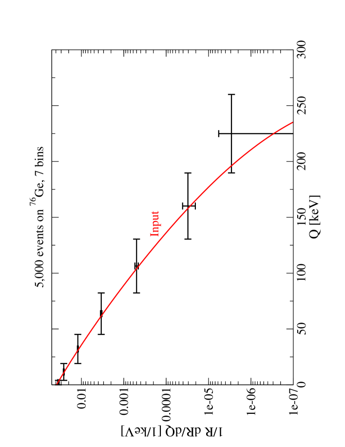
Figure 1: The curve shows the theoretical predicted recoil energy spectrum $(dR/dQ)_{\rm sh}$ for a shifted Maxwellian WIMP velocity distribution, and the Woods–Saxon form factor. The data points with error bars show simulated experimental data produced from this spectrum (5,000 total events, $m_{\chi}$=100 GeV/$c^{2}$, $m_{\rm N}$=70.6 GeV/$c^{2}$ for ${}^{76}{\rm Ge}$, $v_{0}$=220 km/s, $v_{e}$=231 km/s), and galactic escape velocity $v_{\rm esc}=700$ km/s. The vertical error bars show the statistical uncertainties of the measurements, while the horizontal error bars indicate the bin widths.

We had seen at the end of Sec. 2 that the predicted recoil spectrum resembles a falling exponential. This is confirmed in Fig. 1, which shows the predicted recoil spectrum of a 100 GeV WIMP on ⁷⁶Ge, using the Woods–Saxon form factor (29) and the “shifted Maxwellian” velocity distribution of Eq.(19); as usual, we cut the velocity distribution off at a velocity $v_{\rm esc}$, here taken to be 700 km/s, since WIMPs with $v>v_{\rm esc}$ can escape the gravitational well of our galaxy. This figure also shows the result of a simulated experiment, where the exposure time and cross section are chosen such that the expected number of events is 5,000; these have been collected in seven bins in recoil energy.

While an approximately exponential function can be approximated by a linear ansatz, as in Eq.(37), only over a narrow range of $Q$, i.e., for small bin widths, the logarithm of this function can be approximated by a linear ansatz for much wider bins. This corresponds to the ansatz

$$\left(\frac{dR}{dQ}\right)_{n}\equiv\left(\frac{dR}{dQ}\right)_{Q\simeq Q_{n}}\simeq\widetilde{r}_{n}~{}\!{\rm e}^{k_{n}(Q-Q_{n})}\equiv r_{n}~{}\!{\rm e}^{k_{n}(Q-Q_{s,n})}\,.$$ (43)

Here $\widetilde{r}_{n}$ is the recoil spectrum at the point $Q=Q_{n}$,

$$\widetilde{r}_{n}\equiv\left(\frac{dR}{dQ}\right)_{Q=Q_{n}}\,,$$ (44)

while $k_{n}$ is the logarithmic slope of the recoil spectrum in the $n-$th bin.

Our next task is to find estimators for $\widetilde{r}_{n}$ and $k_{n}$ using (simulated) data. Note that for $k_{n}\neq 0$, $\widetilde{r}_{n}$ cannot be estimated from the number of events $N_{n}$ in the $n-$th bin alone. Instead, one has

$$N_{n}=\int_{Q_{n}-b_{n}/2}^{Q_{n}+b_{n}/2}\left(\frac{dR}{dQ}\right)_{n}dQ=b_{n}\widetilde{r}_{n}\left(\frac{\sinh x_{n}}{x_{n}}\right)\,,$$ (45)

where we have introduced the dimensionless quantities

$$x_{n}\equiv\frac{b_{n}k_{n}}{2}\,.$$ (46)

Hence,

$$\widetilde{r}_{n}=\frac{N_{n}}{b_{n}}\left(\frac{x_{n}}{\sinh x_{n}}\right)$$ (47)

depends on $k_{n}$. On the other hand, the second, equivalent expression in Eq.(43) still uses the quantities $r_{n}=N_{n}/b_{n}$ as normalization. Evidently, they describe the spectrum $dR/dQ$ at the shifted points $Q_{s,n}$. Equivalence of the two expressions in Eq.(43) implies

$$Q_{s,n}=Q_{n}+\frac{1}{k_{n}}\ln\left(\frac{\sinh x_{n}}{x_{n}}\right)\,.$$ (48)

The second expression in Eq.(43) thus has the advantage that the prefactor $r_{n}$ can be computed more easily than $\widetilde{r}_{n}$; on the other hand, while the $Q_{n}$ are simply the midpoints of the $n-$th bin, and can thus be chosen at will, the $Q_{s,n}$ are derived quantities; they depend on the logarithmic slopes $k_{n}$, which we haven’t determined yet.

To do so, we again use the average $Q-$value in the $n-$th bin. From Eq.(43) we find:

$$\overline{Q}_{n}-Q_{n}=\frac{\int_{Q_{n}-b_{n}/2}^{Q_{n}+b_{n}/2}(Q-Q_{n})\left(\frac{dR}{dQ}\right)_{n}dQ}{\int_{Q_{n}-b_{n}/2}^{Q_{n}+b_{n}/2}\left(\frac{dR}{dQ}\right)_{n}dQ}=\left(\frac{b_{n}}{2}\right)\coth x_{n}-\frac{1}{k_{n}}\,.$$ (49)

Unfortunately this expression cannot be solved analytically for $k_{n}$. It is, however, straightforward to find $k_{n}$ numerically once $\overline{Q}_{n}$ is known. Alternatively, we can make use of the second moment of the recoil spectrum in the $n-$th bin, defined as

$$\overline{(Q-Q_{n})^{2}}_{n}=\frac{\int_{Q_{n}-b_{n}/2}^{Q_{n}+b_{n}/2}(Q-Q_{n})^{2}\left(\frac{dR}{dQ}\right)_{n}dQ}{\int_{Q_{n}-b_{n}/2}^{Q_{n}+b_{n}/2}\left(\frac{dR}{dQ}\right)_{n}dQ}=\left(\frac{b_{n}}{2}\right)^{2}\left[1-2\left(\frac{\coth x_{n}}{x_{n}}\right)+\frac{2}{x_{n}^{2}}\right]\,.$$ (50)

Multiplying both sides of Eq.(49) with $b_{n}/x_{n}$ and adding to Eq.(50), we can calculate the logarithmic slopes as

$$k_{n}=\frac{8\left(\overline{Q}_{n}-Q_{n}\right)}{b_{n}^{2}-4~{}\!\overline{(Q-Q_{n})^{2}}_{n}}\,.$$ (51)

Note that $k_{n}$ determined either from Eq.(49) or from Eq.(51) is independent of the normalization $r_{n}$ or $\widetilde{r}_{n}$.

In the following we will estimate the logarithmic slopes from Eq.(49), since it simplifies the error analysis somewhat; note that the statistical errors of $\overline{Q}_{n}$ and $\overline{(Q-Q_{n})^{2}}_{n}$ are correlated. Using standard error propagation, we have

$$\sigma^{2}(k_{n})=\sigma^{2}\left(\overline{Q}_{n}-Q_{n}\right)\cdot\left[\frac{d\left(\overline{Q}_{n}-Q_{n}\right)}{dk_{n}}\right]^{-2}\,.$$ (52)

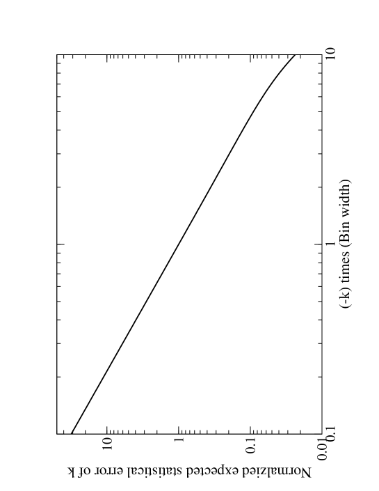
Figure 2: The expected statistical error of our estimator for the logarithmic slope based on Eq.(49) as function of the bin width. The bin width is given in units of the inverse logarithmic slope, and the error is normalized to its value for $b_{n}=-1/k_{n}$. In this calculation we have assumed that the ansatz (43) is exact within the given bin.

The error on the average energy transfer can be estimated directly from the data, using

$$\sigma^{2}\left(\overline{Q}_{n}-Q_{n}\right)=\frac{1}{N_{n}-1}\left[\overline{(Q-Q_{n})^{2}}_{n}-\left(\overline{Q}_{n}-Q_{n}\right)^{2}\right],\,$$ (53)

where now $\overline{(Q-Q_{n})^{2}}_{n}$ is estimated from the data, analogously to the experimental definition of $\overline{Q}_{n}$ in Eq.(36). The second factor in Eq.(52) can be calculated straightforwardly from Eq.(49):

$$\left[\frac{d\left(\overline{Q}_{n}-Q_{n}\right)}{dk_{n}}\right]^{-1}=\frac{k_{n}^{2}}{f(x_{n})}\,,$$ (54)

where we have defined the auxiliary function

$$f(x)=1-\left(\frac{x}{\sinh x}\right)^{2}\,.$$ (55)

For given input values $r_{n},\,k_{n}$ and $b_{n}$, Eqs.(52) and (54) also allow to calculate the expected statistical error of the estimated $k_{n}$, using Eq.(50) to calculate the expected error of $\overline{Q}_{n}-Q_{n}$. The result is shown in Fig. 2. By normalizing the bin width to the inverse slope, and the expected error to its value for a given bin width, the result becomes independent of $r_{n}$, and can in fact be used for all combinations of $k_{n}$ and $b_{n}$. We observe that for small bins, the expected error again scales like $b_{n}^{-1.5}$, just as the expected errors (40) and (42) of our two estimators for the linear slope. If the bin width is significantly larger than the absolute value of the inverse of the logarithmic slope, the error decreases even faster with increasing bin width.

This again argues in favor of using large bins. However, we again have to consider systematic errors. After all, it is quite unlikely that the (as yet unknown) recoil spectrum $dR/dQ$ exactly satisfies our ansatz (43) over an extended range of $Q$. Rather, this ansatz should be considered as the first terms in a Taylor expansion of the logarithm of $dR/dQ$. In this case the next–order term, which contributes $c_{n}(Q-Q_{n})^{2}$ in the exponent, will already modify $\overline{Q}_{n}$. Since we estimate $k_{n}$ from the numerical value of $\overline{Q}_{n}$ using Eq.(49), which is exact only for $c_{n}=0$, any non–zero $c_{n}$ will introduce some systematic error in our estimate of $k_{n}$.

Fortunately much of this error can be absorbed by a simple trick. According to (43) the logarithmic slope is constant over the entire bin, i.e., we could use $k_{n}$ extracted from Eq.(49) as estimate of the logarithmic slope at any point $Q$ between $Q_{n}-b_{n}/2$ and $Q_{n}+b_{n}/2$. Once $c_{n}\neq 0$ the true logarithmic slope will in fact vary with $Q$. However, one may hope that the expectation value of our estimator still reproduces the true logarithmic slope at some value of $Q$ within the $n-$th bin.

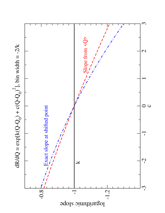
Figure 3: Illustration of the systematic error of our estimator for the logarithmic slope based on Eq.(49). Here we assume that $dR/dQ\propto\exp[k(Q-Q_{0})+c(Q-Q_{0})^{2}]$, i.e., we amend our ansatz (43) by adding a quadratic term to the exponent. The horizontal black line shows the input value of $k$, which now describes the true logarithmic slope only at $Q=Q_{0}$. The dashed (red) line shows the expectation value of our estimator for the logarithmic slope, while the dot–dashed (blue) line shows the true logarithmic slope at the shifted point $Q_{s}$ defined in Eq.(48). The result holds for $k=-1$ and a bin width $b=2$.

This is illustrated by Fig. 3, which shows various evaluations of the logarithmic slope within one bin as function of the quadratic coefficient $c$. The true logarithmic slope at the center of the bin is, of course, still given by $k$, independent of the correction $c$. As argued above, the expectation value of our estimator, shown by the dashed (red) line, does depend on $c$. Note, however, that our estimator comes quite close to the true logarithmic slope at the shifted value $Q_{s}$ defined in Eq.(48), which is shown by the dot–dashed (blue) line; this is true for both signs of $c$. We therefore conclude that we can minimize the leading systematic error by interpreting our estimator of $k_{n}$ as logarithmic slope of the recoil spectrum, not at the center of the bin $Q_{n}$, but at the shifted point $Q_{s,n}$. Note that $Q_{s,n}$ itself depends on $k_{n}$; this, however, does not introduce any additional error, if we simply interpret Eq.(48) as an – admittedly somewhat complicated – prescription for the determination of the $Q-$values where we wish to estimate the logarithmic slope of the recoil spectrum.

Using large bins has a second, obvious disadvantage: the number of bins scales inversely with their size, i.e., by using large bins we’d be able to estimate $f_{1}$ only at a small number of velocities. This can be alleviated by using overlapping bins, or – equivalently – by combining several relatively small bins into overlapping “windows”. This means that a given data point $Q_{n,i}$ may well contribute to several different windows, and hence to the measurement of $f_{1}$ at several values of $v$. This can increase the total amount of information about $f_{1}$ since the only information we use about the data points in a given window is encoded in the average recoil energy in this window. This averaging effectively destroys information. By letting a given data point contribute to several overlapping windows, this loss of information can be reduced.

A final disadvantage of using large bins or windows is that it would lead to a quite large minimal value of $v$ where $f_{1}$ can be reconstructed, simply because the central value $Q_{1}$, and also the shifted point $Q_{s,1}$, of a large first bin would be quite large. This can be again be alleviated by first collecting our data in relatively small bins, and then combining varying numbers of bins into overlapping windows. In particular, the first window would be identical with the first bin.

A final consideration concerns the size of the bins. Choosing fixed bin sizes, and therefore also mostly fixed window sizes, would lead to errors on the estimated logarithmic slopes, and hence also on the estimates of $f_{1}$, that increase quickly with increasing $Q$ or $v$. This is due to the essentially exponential form of the recoil spectrum, which would lead to a quickly falling number of events in equal–sized bins. We found that we get roughly equal errors in all bins if we instead take linearly increasing bins.

These considerations motivate the following set–up for our mock experimental analysis. We start by binning the data, as in Eq.(32), where the bin widths satisfy

$$b_{n}=b_{1}+(n-1)\delta\,;$$ (56)

here the increment $\delta$ satisfies

$$\delta=\frac{2}{B(B-1)}\Big{(}Q_{\rm max}-Q_{\rm min}-Bb_{1}\Big{)}\,,$$ (57)

$B$ being the total number of bins, and $Q_{\rm max,min}$ being the (kinematical or instrumental) extrema of the recoil energy. We then collect up to $n_{W}$ bins into a window, with smaller windows at the borders of the range of $Q$. In the following we use Latin indices $i,~{}j,~{}\cdots$ to label bins, and Greek indices $\mu,~{}\nu,~{}\cdots$ to label windows; later on we will use Latin indices $a,~{}b,~{}\cdots$ to label all events in the sample. For $1\leq\mu\leq n_{W}$ the $\mu-$th window simply consists of the first $\mu$ bins; for $n_{W}\leq\mu\leq B$, the $\mu-$th window consists of bins $\mu-n_{W}+1,~{}\mu-n_{W}+2,\cdots,~{}\mu$; and for $B\leq\mu\leq B+n_{W}-1$, the $\mu-$th window consists of last $n_{W}-\mu+B$ bins. This can also be described by introducing the indices $i_{\mu-}$ and $i_{\mu+}$ which label the first and last bin contributing to the $\mu-$th window, with

$$i_{\mu-}=\left\{\begin{array}[]{ll}1,&\mu\leq n_{W}\\ \mu-n_{W}+1,&\mu\geq n_{W}\end{array}\right.,\ \ \ \ i_{\mu+}=\left\{\begin{array}[]{ll}\mu,&\mu\leq B\\ B,&\mu\geq B\end{array}\right.,\ \ \ (1\leq\mu\leq B+n_{W}-1)\,.$$ (58)

The center of the $i-$th bin is called $Q_{i}$, as before. The total number of windows defined through Eq.(58) is evidently $W=B+n_{W}-1$.

The basic observables needed for the reconstruction of $f_{1}$ are then the number of events $N_{i}$ in the $i-$th bin, as well as the average $\overline{Q}_{i}$ defined as in Eq.(36). From these one easily calculates the number of events per window,

$$N_{\mu}=\sum_{i=i_{\mu-}}^{i_{\mu+}}N_{i}\,$$ (59)

as well as the averages

$$\overline{Q}_{\mu}=\frac{1}{N_{\mu}}\sum_{i=i_{\mu-}}^{i_{\mu+}}N_{i}\overline{Q}_{i}\,.$$ (60)

One drawback of the use of overlapping windows in the analysis is that the observables defined in Eqs.(59) and (60) are all correlated (for $n_{W}\neq 1$). The slope in a given window will again be calculated as in Eq.(49), with “bin” quantities replaced by “window” quantities. We thus need the covariance matrix for the $\overline{Q}_{\mu}-Q_{\mu}$, where $Q_{\mu}$ is the midpoint of the $\mu-$th window; it follows directly from the definition (60):

$${\rm cov}\left(\overline{Q}_{\mu}-Q_{\mu},\overline{Q}_{\nu}-Q_{\nu}\right)=\frac{1}{N_{\mu}N_{\nu}}\sum_{i=i_{\nu-}}^{i_{\mu+}}\bigg{[}N_{i}^{2}\sigma^{2}\left(\overline{Q}_{i}-Q_{i}\right)+N_{i}\left(\overline{Q}_{i}-\overline{Q}_{\mu}\right)\left(\overline{Q}_{i}-\overline{Q}_{\nu}\right)\bigg{]}\,,$$ (61)

where $\sigma^{2}(\overline{Q}_{i}-Q_{i})$ is defined as in Eq.(53). In Eq.(61) we have assumed $\mu\leq\nu$; the covariance matrix is, of course, symmetric. Moreover, the sum is understood to vanish if the two windows $\mu,\ \nu$ do not overlap, i.e., if $i_{\mu+}<i_{\nu-}$.

The ansatz (43) is now assumed to hold over an entire window. We again estimate the prefactor as

$$r_{\mu}=\frac{N_{\mu}}{w_{\mu}}\,,$$ (62)

$w_{\mu}$ being the width of the $\mu-$th window. This implies

$${\rm cov}(r_{\mu},r_{\nu})=\frac{1}{w_{\mu}w_{\nu}}\sum_{i=i_{\nu-}}^{i_{\mu+}}N_{i}\,,$$ (63)

where we have again taken $\mu\leq\nu$. Finally, the mixed covariance matrix is given by

$${\rm cov}\left(r_{\mu},\overline{Q}_{\nu}-Q_{\nu}\right)=\frac{1}{w_{\mu}N_{\nu}}\sum_{i=i_{-}}^{i_{+}}N_{i}\left(\overline{Q}_{i}-\overline{Q}_{\nu}\right)\,.$$ (64)

This sub–matrix is not symmetric under the exchange of $\mu$ and $\nu$. In the definition of $i_{-}$ and $i_{+}$ we therefore have to distinguish two cases:

$${\rm If}\ \mu\leq\nu : \ i_{-}=i_{\nu-}\,,\ i_{+}=i_{\mu+}\,;$$

$${\rm If}\ \mu\geq\nu : \ i_{-}=i_{\mu-}\,,\ i_{+}=i_{\nu+}\,.$$ (65)

As before, the sum in Eq.(64) is understood to vanish if $i_{-}>i_{+}$.

The covariance matrices involving our estimators of the logarithmic slopes $k_{\mu}$, derived from Eq.(49) with $n\rightarrow\mu$ everywhere, can be calculated in terms of the covariance matrices in Eqs.(61) and (64):

$${\rm cov}(k_{\mu},k_{\nu})=\left[\frac{k_{\mu}^{2}k_{\nu}^{2}}{f(x_{\mu})f(x_{\nu})}\right]{\rm cov}\left(\overline{Q}_{\mu}-Q_{\mu},\overline{Q}_{\nu}-Q_{\nu}\right)\,,$$ (66)

where $x_{\mu}$ is as in Eq.(46) with $n\rightarrow\mu$, and the function $f(x)$ has been defined in Eq.(55); and

$${\rm cov}(r_{\mu},k_{\nu})=\left[\frac{k_{\nu}^{2}}{f(x_{\nu})}\right]{\rm cov}\left(r_{\mu},\overline{Q}_{\nu}-Q_{\nu}\right)\,.$$ (67)

We are now ready to put all pieces together to compute the reconstructed velocity distribution and its statistical error. Inserting the ansatz (43) with the substitution $n\rightarrow\mu$ into Eq.(12), one finds the reconstructed velocity distribution

$$f_{1,r}(v_{\mu})={\cal N}\left[\frac{2Q_{s,\mu}r_{\mu}}{F^{2}(Q_{s,\mu})}\right]\left[\frac{d}{dQ}\ln F^{2}(Q)\bigg{|}_{Q=Q_{s,\mu}}-k_{\mu}\right]\,.$$ (68)

Here, $Q_{s,\mu}$ is given by Eq.(48) with $n\rightarrow\mu$, and

$$v_{\mu}=\alpha\sqrt{Q_{s,\mu}},\,$$ (69)

see Eq.(4). Finally, the normalization ${\cal N}$ defined in Eq.(13) can be estimated directly from the data:

$${\cal N}^{-1}=\frac{\alpha}{2}\sum_{a}\frac{1}{\sqrt{Q_{a}}F^{2}(Q_{a})}\,\$$ (70)

where the sum runs over all events in the sample.

Since neighboring windows overlap, the estimates of $f_{1}$ at adjacent values of $v_{\mu}$ are correlated. This is described by the covariance matrix

$${\rm cov}\Big{(}f_{1,r}(v_{\mu}),f_{1,r}(v_{\nu})\Big{)}$$ (71)

$$= \left[\frac{f_{1,r}(v_{\mu})f_{1,r}(v_{\nu})}{r_{\mu}r_{\nu}}\right]{\rm cov}(r_{\mu},r_{\nu})+(2{\cal N})^{2}\left[\frac{Q_{s,\mu}Q_{s,\nu}r_{\mu}r_{\nu}}{F^{2}(Q_{s,\mu})F^{2}(Q_{s,\nu})}\right]{\rm cov}(k_{\mu},k_{\nu})$$

$$~{}~{}~{}~{}~{}~{}-2{\cal N}\left\{\frac{Q_{s,\mu}r_{\mu}}{F^{2}(Q_{s,\mu})}\left[\frac{f_{1,r}(v_{\nu})}{r_{\nu}}\right]{\rm cov}(k_{\mu},r_{\nu})+(\mu\longleftrightarrow\nu)\right\}\,.$$

The covariance matrices involving the normalized counting rates $r_{\mu}$ and logarithmic slopes $k_{\mu}$ have been given in Eqs.(63), (66) and (67). In principle Eq.(71) should also include contributions involving the statistical error of our estimator (70) for ${\cal N}$. However, we find this error, and its correlations with the errors of the $r_{\mu}$ and $k_{\mu}$, to be negligible compared to the errors included in Eq.(71).

We are finally in a position to present some numerical results. We first validate our results by presenting $\chi^{2}_{f}$ distributions, defined via

$$\chi^{2}_{f}\equiv\frac{1}{W}\sum_{\mu,\nu}{\cal C}_{\mu\nu}\left[f_{1,r}(v_{\mu})-f_{1}(v_{\mu})\right]\left[f_{1,r}(v_{\nu})-f_{1}(v_{\nu})\right]\,.$$ (72)

Here $f_{1,r}$ is our estimate (68) of the velocity distribution, $f_{1}$ is the true (input) distribution, and ${\cal C}$ is the inverse of the covariance matrix of Eq.(71). We expect $\chi_{f}^{2}$ to be (roughly) distributed according to the standard $\chi^{2}$ distribution when the results of sufficiently many simulated experiments, with sufficiently many events per experiment, are analyzed.

Figs. 4 show $\chi^{2}_{f}$ distributions for 5,000 simulated experiments, with on average 500 (top) and 5,000 (bottom) events per experiments. Note that the actual number of events in a given simulated experiment varies according to the Poisson distribution; otherwise one would introduce an artificial correlation between the normalized counting rates $r_{i}$ in different bins. Moreover, the number of bins has been fixed a priori in these analyses. The last bin is typically empty, and has therefore been ignored in the analysis. This also reduces the number of windows used in the analysis by one, i.e., the upper (lower) frame shows results for $W=6$ ($W=8$).

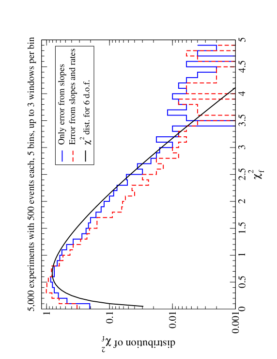
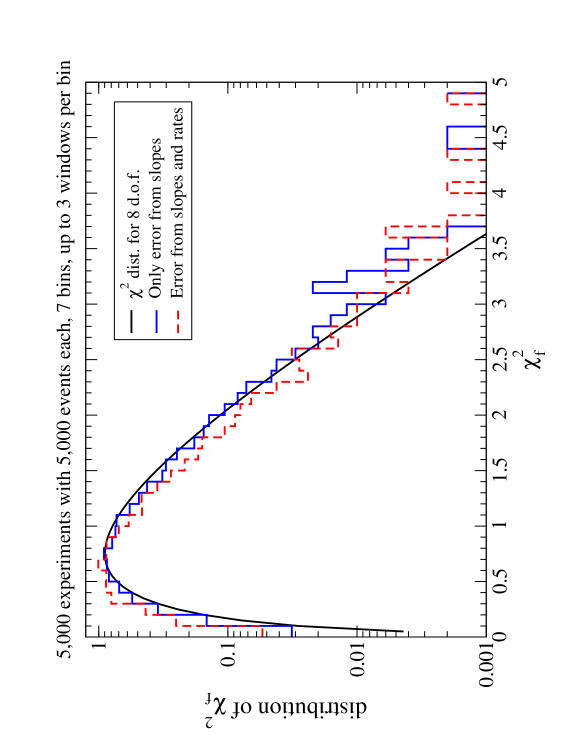
Figure 4: The distribution of $\chi^{2}_{f}$ defined in Eq.(72) over 5,000 simulated experiments, with on average 500 (top) and 5,000 (bottom) events per experiment. The solid (blue) and dashed (red) histograms have been obtained by estimating the covariance matrix for the reconstructed velocity distribution excluding (including) the statistical errors on the number of events in the windows. The smooth (black) curves show the theoretical $\chi^{2}$ distributions for the appropriate numbers of degrees of freedom. Parameters are as in Fig. 1.

The two histograms in each figure differ by the number of terms that have been included in the estimate of the covariance matrix for $f_{1,r}$. The solid (blue) histograms have been obtained by only including the second term in Eq.(71), while the dashed (red) histograms also include the other terms, which are due to the statistical errors on the rescaled event numbers $r_{\mu}$. We note that including these terms on average leads to a slight overestimate of the true error of $f_{1,r}$, i.e., the average of $\chi_{f}^{2}$ is somewhat smaller than unity. This is partly due to the fact that we have ignored the error on the normalization ${\cal N}$, which is correlated quite strongly with the errors on the $r_{\mu}$.

The lower figure demonstrates that for an average of 5,000 events per experiment the distribution of $\chi_{f}^{2}$ values becomes quite similar to the well–known $\chi^{2}$ distribution, shown by the smooth curve. At least two effects contribute to the difference. First, we heavily relied on Gaussian error propagation in our estimate (71) of the covariance matrix of the reconstructed velocity distribution. This is essentially a Taylor expansion, including only the first non–trivial term. It therefore becomes exact only in the limit of small errors, i.e., for large numbers of events in a given window. Since the recoil spectrum is falling essentially exponentially, this condition is practically always violated at least in the last bin(s), see Fig. 1. We discard windows containing less than 3 events, but it is clear that this at best alleviates the problem. In the case at hand, this evidently results in an overestimate of the true error. Secondly, our estimator (68) for the velocity distribution relies on the estimate of the logarithmic slopes $k_{\mu}$, which in turn is based on Eq.(49). As illustrated in Fig. 3 this estimate of $k_{\mu}$ in general has some systematic error, which would tend to increase $\chi_{f}^{2}$. However, this figure also led us to expect small systematic errors if $k_{\mu}$ is interpreted as estimator of the logarithmic slope at the shifted points $Q_{s,\mu}$. Indeed, as stated above, the total expression (71) somewhat overestimates the true error even in the lower frame of Figs. 4, which assumes a large number of events but uses a rather small number of bins, which thus have to be quite large. Had we instead interpreted $k_{\mu}$ as estimator of the slope at $Q_{\mu}$, the average $\chi_{f}^{2}$ would be about 2.9, indicating that the systematic error would have dominated.

Figs. 4 also show an excess of simulated experiments with rather large values of $\chi_{f}^{2}$ if the covariance matrix for $f_{1,r}$ is estimated based on the errors on the $k_{\mu}$ only. This is true also for the upper frame, even though in this case the average value of $\chi_{f}^{2}$ is only about 0.93. To be conservative, from now on we therefore take the full Eq.(71) as our estimator of the covariance matrix of $f_{1,r}$, leading to average $\chi_{f}^{2}=0.78\ (0.94)$ for the upper (lower) frame of Figs. 4.

In Figs. 5 we show results for the reconstructed velocity distribution, for “typical” simulated experiments with 500 (top) and 5,000 (bottom) events. In the top frame we choose $B=5$ bins, the first bin having a width $b_{1}=8$ keV, and combine up to three bins into a window. Since the last bin is in fact empty, this leaves us with $W=6$ windows, i.e., we can determine $f_{1}$ for six discrete values of the WIMP velocity $v$; recall that these “measurements” of $f_{1}$ are correlated, as indicated by the horizontal bars in the figure. In the lower frame we choose $B=10$ bins with $b_{1}=10$ keV, and combine up to four bins into one window. The bins are thus significantly smaller than in the upper frame. As a result, the last two bins are now (almost) empty, leaving us with $W=11$ windows.

Figs. 5 indicate that one will need at least a few hundred events for a meaningful direct reconstruction of $f_{1}$. Recall that $f_{1}$ is normalized to unity. The overall magnitude of $f_{1}$ is therefore essentially fixed by the range of observed $Q-$values; only the shape of this distribution then remains to be determined. One measure of the information content of the reconstructed $f_{1,r}$ is therefore the confidence level with which one can exclude a constant $f_{1}$.

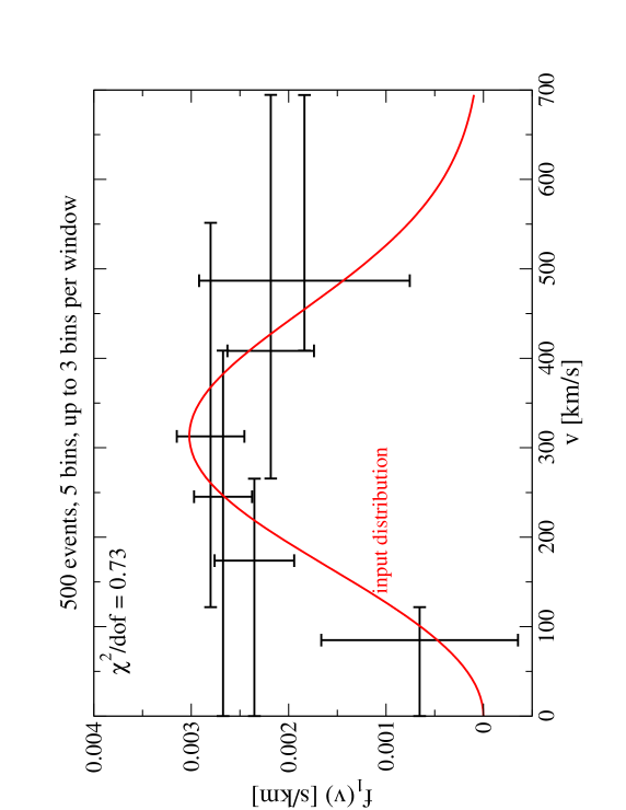
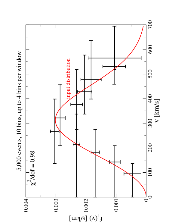
Figure 5: The WIMP velocity distribution reconstructed from a “typical” experiment with 500 (top) and 5,000 (bottom) events. The smooth curves show the input distributions, which are based on Eq.(19). The vertical error bars show the square roots of the diagonal entries of the covariance matrix (71); the horizontal bars show the size of the window used in deriving the given value of $f_{1,r}$. The overlap of these horizontal bars thus shows the range over which the values of $f_{1,r}$ are correlated. Parameters as in Fig. 1.

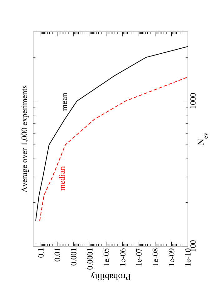
Figure 6: Estimates of the probability that the reconstructed velocity distribution is compatible with being constant, as a function of the average number of events per experiment. These results are for optimal combinations of $B,\ b_{1}$ and $n_{W}$; they have been obtained by averaging over 1,000 simulated experiments. The solid (black) and dashed (red) curves show the mean and median values of the probability. Parameters as in Fig. 1.

In Fig. 6 we show one minus this confidence level, i.e., the probability that a reconstructed velocity distribution is compatible with a constant. This has been estimated by defining a $\chi_{f}^{2}$ variable as in Eq.(72) for the hypothesis $f_{1}=$ const., and integrating the theoretical $\chi^{2}$ distribution over the range $\chi^{2}>\chi_{f}^{2}$. Here the constant has been chosen as $1/(v_{\rm max}-v_{\rm min})$, where $v_{\rm min,max}$ have been calculated as in Eq.(4) using the largest and smallest recoil energy, respectively, that has been measured in a given experiment. Since this probability differs quite widely from one (simulated) experiment to the next, we show both the mean and the median probability. We see that we’ll need at least 200 events if we want to reject the hypothesis of a constant $f_{1}$ at the 90% C. L. (on average). The confidence level then increases very quickly as additional events are added; by the time 1,000 events have been accumulated, we can be quite sure that a constant $f_{1}$ can be excluded with high confidence.

$N_{rmev}$	$B$	$b_{1}$ [keV]	$n_{W}$	mean $P$	median $P$	$\langle\Sigma\rangle$	$\langle\chi_{f}^{2}\rangle$
500	5	30	3	0.032	$3.2\cdot 10^{-3}$	145	0.78
500	5	30	2	0.08	0.02	107	0.77
500	5	30	1	0.38	0.34	19	0.88
500	5	30	4	$9.0\cdot 10^{-3}$	$5.0\cdot 10^{-4}$	165	1.3
500	2	100	1	0.08	0.03	80	0.6
5,000	6	20	3	$2.8\cdot 10^{-23}$	$1.2\cdot 10^{-40}$	1,360	1.03
5,000	6	30	3	$1.7\cdot 10^{-26}$	$2.0\cdot 10^{-42}$	1,380	1.28
5,000	10	10	4	$2.9\cdot 10^{-21}$	$1.0\cdot 10^{-37}$	1,520	0.85
5,000	10	10	3	$3.5\cdot 10^{-11}$	$2.5\cdot 10^{-26}$	1,190	0.85
5,000	10	10	2	$9.5\cdot 10^{-7}$	$5.4\cdot 10^{-12}$	490	0.88
5,000	10	10	1	0.02	$6.7\cdot 10^{-4}$	48	0.93

Table 1: This table illustrates how the binning, and in particular the combination of bins into “windows”, affects the information that can be gleaned from the reconstructed WIMP velocity distribution. The first four columns show the average number of events in a given experiment, the number of bins, the size of the first bin in keV, and the number of bins per window. The remaining four columns show the mean and median probability that the reconstructed $f_{1}$ is compatible with a constant, the mean of the quantity $\Sigma$ defined in Eq.(73), and the average $\chi_{f}^{2}$ of Eq.(72).

This confidence level, as well as more general measures of the information that can be extracted from a given experiment, depend on the choices of $B,b_{1}$ and, in particular, $n_{W}$. This is illustrated in Table 1, which shows results for different combinations of $B,\,b_{1}$ and $n_{W}$ for 500 (first five rows) and 5,000 (last six rows) expected events per experiment. Here the mean and median probabilities are the same as in Fig. 6. In addition we show the mean of the quantity $\Sigma$, defined as

$$\Sigma=\sum_{\mu,\nu}{\cal C}_{\mu\nu}f_{1,r}(v_{\mu})f_{1,r}(v_{\nu})\,.$$ (73)

Formally $\Sigma$ determines the significance with which the hypothesis $f_{1}=0$ can be rejected. Since $f_{1}$ is normalized, this hypothesis is unphysical. Nevertheless $\Sigma$ can be regarded as a measure of the information content of a set of reconstructed $f_{1,r}(v_{\mu})$; in the absence of correlations, it becomes the sum over the inverse squares of the relative errors. Note that, in contrast to $\chi_{f}^{2}$, $\Sigma$ does not have a $1/W$ factor in front; after all, by adding more windows we also add more values $v_{\mu}$ at which $f_{1}$ is determined, which can increase the information content.

The first four rows, as well as the last four rows, show the effect of varying $n_{W}$, the maximal number of bins that are collected in a window. We see that there is an optimal choice for this quantity. Reducing $n_{W}$ leads to loss of information, as indicated by greatly increased values for the probability that $f_{1,r}$ is compatible with $f_{1}$ being constant as well as reduced values of $\Sigma$. On the other hand, making the windows too large introduces too large systematic uncertainties in the estimates of the logarithmic slopes $k_{\mu}$, which in turn leads to too large average values of $\chi_{f}^{2}$. This is illustrated by rows four and seven, which have large windows due to our choice of a large $n_{W}$ (row 4) or a large $b_{1}$ (row 7).

The table also shows that the choice of $b_{1}$ has some impact on the confidence level with which the hypothesis of a constant $f_{1}$ can be rejected. We saw in Figs. 5 that our input $f_{1}$ has a broad maximum at $v\simeq 300$ km/s. Rejection of the hypothesis of a constant $f_{1}$ is therefore optimized by maximizing the information about the outer reaches of $f_{1}$. Getting accurate information about $f_{1}$ at large velocities is very difficult; this would need a large number of events at large $Q$, where the counting rate is very small. This leaves the region of small WIMP velocity. By choosing a large first bin, one greatly reduces the error on $f_{1,r}$ in this first bin, which is also the first window; this was illustrated in Fig. 2. In fact, for 500 events and $n_{W}=1$ one can formally maximize the confidence level with which a constant $f_{1}$ can be rejected by considering only two bins, and making the first bin very large; this is shown in the fifth row. Note that this leads to an average $\chi_{f}^{2}$ well below unity, indicating that in spite of the large bins, systematic errors are still insignificant. However, we note that in this case our assumption that the error on ${\cal N}$ is negligible is clearly not justified, since ${\cal N}$ receives almost its entire contribution from the large first bin. By including the error on $r_{1}$ but ignoring the (strongly correlated!) error on ${\cal N}$ we clearly over–estimate the total statistical error in this case. Recall also that a large first bin leads to a large value for the smallest velocity, $v_{1}$, where $f_{1}$ is determined.

Our “figure of merit” $\Sigma$ is less dependent on the details of binning, although, as stated earlier, it does strongly benefit from combining several bins into windows. We also note that the optimal achievable $\Sigma$ is essentially proportional to the number of events in the sample. This is expected, since $\Sigma$ is something like an inverse squared relative error.

3.3 Determining moments of $f_{1}$

We saw in the previous subsection that a direct reconstruction of the WIMP velocity distribution $f_{1}$ will only be possible once several hundred elastic nuclear recoil events have been collected. This is a tall order, given that not a single such event has so far been detected (barring the possible DAMA observation). The basic reason for the large required event sample is that, $f_{1}$ being a normalized distribution, only information on the shape of $f_{1}$ is meaningful. In order to obtain such shape information via direct reconstruction, we have to separate the events into several bins or windows. Moreover, each window should contain sufficiently many events to allow an estimate of the slope of the recoil spectrum in this window.

On the other hand, at the end of Sec. 2 we also gave expressions for the moments of $f_{1}$. With the exception of the moment with $n=-1$, these are entirely inclusive quantities, i.e., each moment is sensitive to the entire data set; no binning is required, nor do we need to determine any slope (with one possible minor exception; see below). It thus seems reasonable to expect that one can obtain meaningful information about these moments with fewer events.

An independent motivation for the determination of these moments is that they are sensitive also to $f_{1}$ at large values of the WIMP velocity $v$. We saw above that direct reconstruction of $f_{1}$ at large $v$ is very difficult, due to the small number of events expected in this region. Moreover, a delta–function–like contribution to $f_{1}$ at the highest velocity, $v=v_{\rm esc}$ is very difficult to detect using direct reconstruction; such a contribution is expected in “late infall” models of galaxy formation [11].

The experimental implementation of Eq.(15) is quite straightforward. For $Q_{\rm thre}=0$, the normalization ${\cal N}$ has already been given in Eq.(70). The case of non–vanishing threshold energy $Q_{\rm thre}$ can be treated straightforwardly, using Eq.(17). To that end we need to estimate the recoil spectrum at the threshold energy. One possibility would be to choose an artificially high value of $Q_{\rm thre}$, and simply count the events in a bin centered on $Q_{\rm thre}$. However, in this case the events with $Q<Q_{\rm thre}$ would be left out of the determination of the moments. We therefore prefer to keep $Q_{\rm thre}$ as small as experimentally possible, and to estimate the counting rate at threshold using the ansatz (43). Since we need the recoil spectrum only at this single point, we only have to determine the quantities $r_{1}$ and $k_{1}$ parameterizing $dR/dQ$ in the first bin; this can be done as described in the previous subsection, without the need to distinguish between bins and “windows”. Introducing the shorthand notation

$$r_{\rm thre}\equiv\left(\frac{dR}{dQ}\right)_{Q=Q_{\rm thre}}\,,$$ (74)

the resulting error can be written as

$$\sigma^{2}(r_{\rm thre})=r_{\rm thre}^{2}\left\{\frac{\sigma^{2}(r_{1})}{r_{1}^{2}}+\left[Q_{\rm thre}-Q_{s,1}-k_{1}\left(\frac{\partial Q_{s,1}}{\partial k_{1}}\right)\right]^{2}\sigma^{2}(k_{1})\right\}\,.$$ (75)

The squared errors for $r_{1}$ and $k_{1}$ are simply the corresponding diagonal entries of the respective covariance matrices given in Eqs.(63) and (66). Finally, the definition (48) of $Q_{s,1}$ implies

$$Q_{s,1}+k_{1}\left(\frac{\partial Q_{s,1}}{\partial k_{1}}\right)=Q_{1}-\frac{1}{k_{1}}+\left(\frac{b_{1}}{2}\right)\coth x_{1}\,,$$ (76)

where $x_{1}=b_{1}k_{1}/2$ as before and $Q_{1}$ is the central $Q-$value in the first bin. It should be noted that the first term in Eq.(15) is negligible for all $n\geq 1$ if $Q_{\rm thre}\simeq 1$ keV; however, even for this low threshold energy it contributes significantly to the normalization constant ${\cal N}$, as described by Eq.(17). Of course, the first term in Eq.(15) always dominates for $n=-1$. This is not surprising, since the very starting point of our analysis, Eq.(1), already shows that the counting rate at $Q_{\rm thre}$ is proportional to the “minus first” moment of the velocity distribution.

The integral appearing in Eq.(15) can be estimated through the sum

$$I_{n}=\sum_{a}\frac{Q_{a}^{(n-1)/2}}{F^{2}(Q_{a})}\,,$$ (77)

see Eq.(70). Since all $I_{n}$ are determined from the same data, they are correlated, with

$${\rm cov}(I_{n},I_{m})=\sum_{a}\frac{Q_{a}^{(n+m-2)/2}}{F^{4}(Q_{a})}\,.$$ (78)

This can e.g. be seen by writing Eq.(77) as a sum over narrow bins, such that the recoil spectrum within each bin can be approximated by a constant. Each term in the sum would then have to be multiplied with the number of events in this bin; Eq.(78) then follows from standard error propagation. Note that, when re–converted into an integral, the expression for ${\rm cov}(I_{0},I_{0})$ will diverge logarithmically for $Q_{\rm thre}\rightarrow 0$; equivalently, the numerical estimate of this entry can become very large if the sample contains events with very small $Q-$values. Our numerical results presented below have therefore been obtained with $Q_{\rm thre}=1$ keV; many existing experiments in fact require significantly larger energy transfers in their definition of a WIMP signal.

We also need the correlation between the errors on the estimate of the recoil spectrum at $Q=Q_{\rm thre}$ and the integrals $I_{n}$. It is clear that these quantities are correlated, since the former is estimated from all events in the first bin, which of course also contribute to the latter. We estimate these correlations again using the ansatz (43), which makes the following prediction for the contribution of the first bin to the integrals:

$$I_{n,1}=r_{1}\int_{Q_{\rm thre}}^{Q_{\rm thre}+b_{1}}\left[\frac{Q^{(n-1)/2}}{F^{2}(Q)}\right]{\rm e}^{k_{1}(Q-Q_{s,1})}\,dQ\,.$$ (79)

This immediately implies $\partial I_{n,1}/\partial r_{1}=I_{n,1}/r_{1}$, and

$$\frac{\partial I_{n,1}}{\partial k_{1}}=I_{n+2,1}-\left[Q_{s,1}+k_{1}\left(\frac{\partial Q_{s,1}}{\partial k_{1}}\right)\right]I_{n,1}\,$$ (80)

see Eq.(76). Note that the $I_{n,1}$ and $I_{n+2,1}$ in Eq.(80) are evaluated as in Eq.(77), with the sum extending only over events in the first bin. The correlation we’re after is then given by

$${\rm cov}(r_{\rm thre},I_{n})$$

$$= r_{\rm thre}~{}\!I_{n,1}\left\{\frac{\sigma^{2}(r_{1})}{r_{1}^{2}}+\left[\frac{I_{n+2,1}}{I_{n,1}}-Q_{s,1}-k_{1}\left(\frac{\partial Q_{s,1}}{\partial k_{1}}\right)\right]\left[Q_{\rm thre}-Q_{s,1}-k_{1}\left(\frac{\partial Q_{s,1}}{\partial k_{1}}\right)\right]\!\sigma^{2}(k_{1})\right\}\,.$$

These ingredients allow us to compute the covariance matrix for our estimates of the moments of the velocity distribution:

$${\rm cov}\Big{(}\langle v^{n}\rangle,\langle v^{m}\rangle\Big{)}$$ (82)

$$= {\cal N}_{\rm m}^{2}\bigg{[}\langle v^{n}\rangle\langle v^{m}\rangle{\rm cov}(I_{0},I_{0})+\alpha^{n+m}(n+1)(m+1){\rm cov}(I_{n},I_{m})$$

$$~{}~{}~{}~{}~{}~{}~{}~{}-\alpha^{m}(m+1)\langle v^{n}\rangle{\rm cov}(I_{0},I_{m})-\alpha^{n}(n+1)\langle v^{m}\rangle{\rm cov}(I_{0},I_{n})$$

$$~{}~{}~{}~{}~{}~{}~{}~{}~{}~{}~{}~{}~{}~{}+D_{n}D_{m}\sigma^{2}(r_{\rm thre})-\Big{(}D_{m}\langle v^{n}\rangle+D_{n}\langle v^{m}\rangle\Big{)}{\rm cov}\left(r_{\rm thre},I_{0}\right)\Bigg{.}$$

$$~{}~{}~{}~{}~{}~{}~{}~{}~{}~{}~{}~{}~{}~{}~{}~{}~{}~{}~{}~{}+\alpha^{m}(m+1)D_{n}{\rm cov}(r_{\rm thre},I_{m})+\alpha^{n}(n+1)D_{m}{\rm cov}(r_{\rm thre},I_{n})\bigg{]}\,.$$

Here we have introduced the modified normalization

$${\cal N}_{\rm m}\equiv\left(\frac{\alpha}{2}\right){\cal N}\,,$$ (83)

which exploits the partial cancellation of the $\alpha$ factors between Eqs.(15) and (17), and the quantities

$$D_{n}\equiv\frac{1}{{\cal N}_{\rm m}}\left(\frac{\partial\langle v^{n}\rangle}{\partial r_{\rm thre}}\right)=\frac{2}{F^{2}(Q_{\rm thre})}\left(\alpha^{n}Q_{\rm thre}^{(n+1)/2}-\sqrt{Q_{\rm thre}}~{}\!\langle v^{n}\rangle\right)\,.$$ (84)

In our numerical simulations we find that Eq.(77) indeed reproduces the “exact” (input) values of the $I_{n}$ if one includes sufficiently many events. In this case it does not matter whether one considers a single experiment with a large number of events, or averages over many simulated experiments with a relatively small number of events. However, in the second case the average values of the reconstructed moments do not exactly converge to the input values. In order to understand this, consider the simple case $Q_{\rm thre}=0$. The moments are then proportional to the ratio $I_{n}/I_{0}$, see Eqs.(15) and (17). The distortion arises because $\langle I_{n}/I_{0}\rangle\neq\langle I_{n}\rangle/\langle I_{0}\rangle$, where the averaging is over many simulated experiments. In Appendix B we show how this can be corrected using Taylor expansion to second order. The leading correction terms for small $Q_{\rm thre}$ and not very large first bin are

$$\delta\langle v^{n}\rangle = \alpha^{n}{\cal N}_{\rm m}^{2}\Bigg{\{}(n+1)\bigg{[}{\rm cov}(I_{0},I_{n})-{\cal N}_{\rm m}I_{n}{\rm cov}(I_{0},I_{0})\bigg{]}$$ (85)

$$~{}~{}~{}~{}~{}~{}~{}~{}~{}~{}~{}~{}+2\left[\frac{Q_{\rm thre}^{(n+1)/2}}{F^{2}(Q_{\rm thre})}\right]\bigg{[}{\rm cov}(r_{\rm thre},I_{0})-r_{\rm thre}{\cal N}_{\rm m}{\rm cov}(I_{0},I_{0})\bigg{]}\Bigg{\}}\,,$$

the second line is significant only for $n=-1$. Note that this correction becomes very small if the statistical errors on the $I_{n}$ as well as on $r_{\rm thre}$ become small.

With this correction, the reconstructed $\langle v^{n}\rangle$ indeed closely reproduce the input values after averaging over sufficiently many experiments, even if the number of events in a given experiment is small. However, the numerical analysis revealed a number of additional problems. These can be understood from the observation that the $I_{n}$ in Eq.(77), and even more the entries in their covariance matrix (78), receive significant contributions from large $Q$ values, where the counting rate itself is already very small.

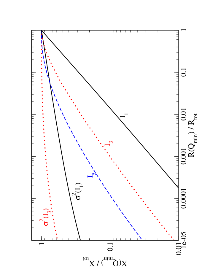
Figure 7: This figure has been obtained by introducing an artificial lower bound $Q_{\rm min}$ in the counting rate as well as in the definition of the integrals $I_{n}$. The $x-$axis shows the counting rate for different $Q_{\rm min}$, where small $R(Q_{\rm min})$ corresponds to large $Q_{\rm min}$. The $y-$axis shows the impact of varying $Q_{\rm min}$ on $I_{1}$ (solid, black), $I_{3}$ (dotted, red) and $I_{5}$ (dashed, blue); the upper curve of a given pattern refers to ${\rm cov}(I_{n},I_{n})$. The values of the parameters are as in Fig. 1. See the text for further details.

This is illustrated in Fig. 7. The $x-$axis shows the quantity

$$R(Q_{\rm min})\equiv\int_{Q_{\rm min}}^{Q_{\rm max}}\left(\frac{dR}{dQ}\right)dQ\,,$$ (86)

divided by the total counting rate $R\equiv R(Q_{\rm min}=0)$. Here, $Q_{\rm max}$ is the kinematic maximum of $Q$ for given input parameters, and $Q_{\rm min}$ is varied freely between 0 and $Q_{\rm max}$. The $y-$axis shows analogously the contributions to some $I_{n}$ (lower curves) and to the corresponding diagonal elements of the covariance matrix, i.e., the squared errors (upper curves), that come from the region $Q>Q_{\rm min}$. In the latter case we have converted the sums in Eq.(78) back into integrals. The figure shows that the region of $Q-$values that contributes 99% of the counting rate only contributes about 92% to $I_{1}$, 73% to $I_{3}$ and 51% to $I_{5}$; for the given input parameters, this corresponds to the region $Q\leq 103$ keV. Even worse, this region only contributes about 35% to ${\rm cov}(I_{1},I_{1})$ and 5% to ${\rm cov}(I_{3},I_{3})$! This implies that an experiment collecting only a small number of events will typically underestimate $\langle v^{n}\rangle$ and, especially, its error; the problem will become worse with increasing $n$. On the other hand, as mentioned above, when averaged over sufficiently many experiments, our estimates for the $I_{n}$ do reproduce the true (input) values. This implies that occasionally an experiment will greatly overestimate the $I_{n}$, the problem again getting worse for larger $n$.

Our numerical analysis also shows that, after averaging over (very) many experiments, Eq.(78) reproduces the mean square deviation between our estimated $I_{n}$ and the true (input) value. Nevertheless, we just saw that in most cases this error is being underestimated. In order to be conservative, we therefore added “the error on the error” to the diagonal entries of the covariance matrix; the off–diagonal entries are then scaled up such that the correlation matrix remains unaltered. The squared “error on the error” is defined as

$$\sigma^{2}\big{(}{\rm cov}(I_{n},I_{n})\big{)}=\sum_{a}\frac{Q_{a}^{2n-2}}{F^{8}(Q_{a})}\,.$$ (87)

With this modification, the average $\chi^{2}$, again averaged over many experiments, is in the vicinity of unity at least for the first few moments.

Another problem is that the errors of the $I_{n}$ are very highly correlated. This can also be understood from Fig. 7: A single event at high $Q$ will contribute greatly to all moments with sufficiently large $n$. Numerically we find correlations of more than 98% between $\langle v^{n}\rangle$ and $\langle v^{n+1}\rangle$ for all $n\geq 2$; the correlation between $\langle v\rangle$ and $\langle v^{3}\rangle$ still amounts to more than 87%. This implies that the higher moments unfortunately add only little to the available information. Worse, attempting to include high moments in a $\chi^{2}$ fit often leads to numerical instabilities; recall that a covariance matrix containing 100% correlated entries become singular, i.e., can no longer be inverted. In practice only the moments with $n~{}\!\>\raisebox{-2.15277pt}{$\stackrel{{\scriptstyle\textstyle<}}{{\sim}}$}\>~{}\!3$ therefore seem to be useful.

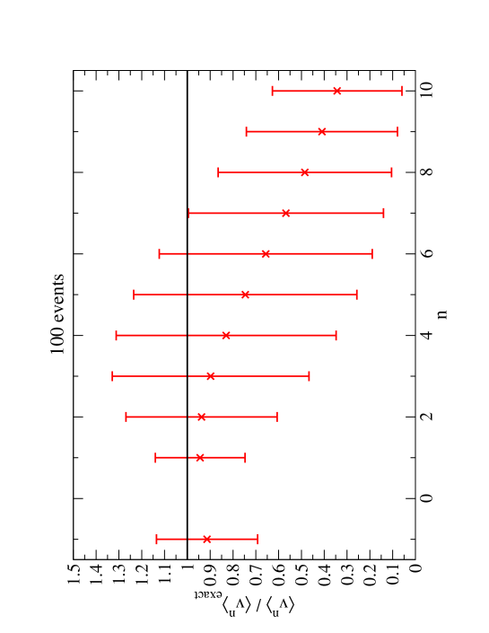
Figure 8: Estimated moments, and their errors, for a “typical” simulated experiment with 100 events; recall that the errors are strongly correlated. Parameters are as in Fig. 1.

We are now ready to present some representative numerical results. Fig. 8 shows the first 10 moments reconstructed with 100 events, using our standard input parameters (see Fig. 1). The estimated values of the moments have been divided by the true values. We see that in this “typical” example the high moments are indeed underestimated. We also see that the estimated relative errors at first increase with increasing $n$; this reproduces correctly the trend of the actual deviation of the estimated moments from the exact values. However, even after adding “the error on the error”, we find that the relative errors start to decline again for $n>6$. This effect is probably entirely spurious; recall that the errors are likely to be even more underestimated than the moments themselves. Nevertheless we find it encouraging that already with 100 events a couple of moments can be determined with errors of about 15%.

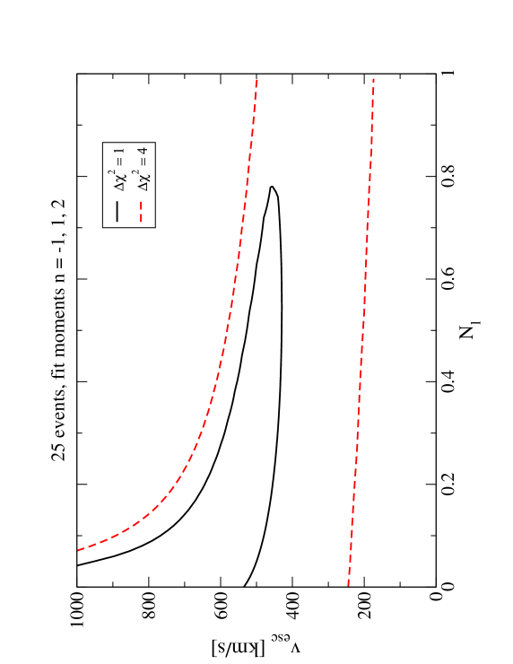
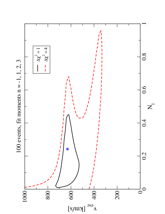
Figure 9: $\chi^{2}$ contours, calculated from 3 (top) and 4 (bottom) moments, in the plane spanned by the normalization of the “late infall” component and the galactic escape velocity, for typical experiments with 25 (top) and 100 (bottom) events. In the upper frame the minimal $\chi^{2}$ value is close to the input values $N_{l}=0,\,v_{\rm esc}=700$ km$/$s; in the lower frame, the location of the minimal $\chi^{2}$ is indicated by the star. Parameters are as in Fig. 1.

Figs. 9 show a example of the information that might be gleaned from analyses of reconstructed moments of the WIMP velocity distribution. Here we attempt to constrain a possible “late infall” component in $f_{1}$ [11], defined by the ansatz

$$f_{1}(v;v_{\rm esc},N_{l})=N_{s}f_{1,{\rm sh}}(v)\theta(v_{\rm esc}-v)+N_{l}\delta(v-v_{\rm esc})\,.$$ (88)

Here $f_{1,{\rm sh}}$ is the standard “shifted Gaussian” distribution (19). As before, we have multiplied it with a cut–off at $v_{\rm esc}$. In addition, we introduce a contribution of WIMPs with fixed velocity, which we set equal to $v_{\rm esc}$; these WIMPs are just falling into our galaxy. $N_{l}$ and $v_{\rm esc}$ are our free parameters; $N_{s}$ is then chosen such that the total $f_{1}$ is normalized to unity. We then plot contours of $\delta\chi^{2}$, defined as the deviation of $\chi^{2}$ from its minimal value, where $\chi^{2}$ is defined as

$$\chi^{2}=\sum_{m,n}\left[\langle v^{m}\rangle_{r}-\langle v^{m}\rangle(v_{\rm esc},N_{l})\right]{\cal D}_{mn}\left[\langle v^{n}\rangle_{r}-\langle v^{n}\rangle(v_{\rm esc},N_{l})\right]\,;$$ (89)

here $\langle v^{n}\rangle_{r}$ are the reconstructed moments in our mock experiment, $\langle v^{n}\rangle(v_{\rm esc},N_{l})$ are the predictions for these quantities based on Eq.(88), and ${\cal D}$ is the inverse of the covariance matrix (82).

Figs. 9 show a strong degeneracy in the fit. If the galactic escape velocity $v_{\rm esc}$ is kept fixed at its input value of 700 km/s, a quite significant upper bound on the normalization $N_{l}$ of the late infall component could be derived already from our simulated experiment with 25 events. However, if $v_{\rm esc}$ is kept free, no significant upper bound can be derived even from the simulated experiment with 100 events. Note that the two experiments have been simulated independently, i.e., the 25 events used for the analysis in the upper frame are not part of the 100 events used in the lower frame. The simulated experiment with 100 events was a bit “unlucky” in that the input values lie just outside the $\Delta\chi^{2}=1$ contour. As a result, the upper bound on $N_{l}$ for fixed $v_{\rm esc}=700$ km/s actually comes out a little worse in this case than in the experiment with only 25 events. This is in spite of the fact that the larger data sample allowed us to include one more moment in the fit.

Note that, according to the definition (88), all WIMPs in our galactic neighborhood have velocity $v<v_{\rm esc}$. This implies that a lower bound on $v_{\rm esc}$ can be derived from the highest observed $Q-$value, $v_{\rm esc}>\alpha\sqrt{Q_{+}}$, see Eq.(4). Unfortunately for our standard set of input parameters, this method on average only yields lower bounds of about 400 (460) km/s for experiments with 25 (100) events. Even the experiment with 100 events would then still allow 60% of all WIMPs to originate from a late infall component; this is to be compared with the theoretical expectation $N_{l}~{}\!\>\raisebox{-2.15277pt}{$\stackrel{{\scriptstyle\textstyle<}}{{\sim}}$}\>~{}\!10\%$. Finally, we note that for $N_{l}=0$, it will be essentially impossible to derive a meaningful upper bound on $v_{\rm esc}$ from these experiments: because the original “shifted Gaussian” velocity distribution is already very small at our input value $v_{\rm esc}=700$ km/s, increasing $v_{\rm esc}$ has essentially no effect on the measured recoil spectrum.

4 Summary and Conclusions

In this paper, we have developed methods that allow to extract information on the WIMP velocity distribution from the recoil energy spectrum $dR/dQ$ measured in elastic WIMP–nucleus scattering experiments. In the long term this information can be used to test or constrain models of the dark halo of our galaxy; this information would complement the information on the density distribution of WIMPs, which can be derived e.g. from measurements of the galactic rotation curve.

To this end, in Sec. 2 we derived expressions that allow to directly reconstruct the normalized one–dimensional velocity distribution function of WIMPs, $f_{1}(v)$, given an expression (e.g., a fit to data) for the recoil spectrum. We have also derived formulae for the moments of $f_{1}$. All these expressions are independent of the as yet unknown WIMP density near the Earth as well as of the WIMP–nucleus cross section; the only information about the nature of the WIMP that is needed is its mass.

Furthermore, in Sec. 3 we have developed methods that allow to apply our expressions directly to data, without the need to fit the recoil spectrum to a functional form. We found that a good variable that allows direct reconstruction of $f_{1}$ is the average recoil energy in a given bin (or “window”; see Sec. 3.2). This average energy is sensitive to the slope of the recoil spectrum, which is the quantity we need to reconstruct $f_{1}$. We carefully analyzed the statistical errors. Unfortunately we found that several hundred events will be needed for this method to be able to extract meaningful information on $f_{1}$. This is partly due to the fact that $f_{1}(v)$ is normalized, i.e., only the shape of this distribution contains meaningful information, and partly because this shape depends on the slope of the recoil spectrum, which is intrinsically difficult to determine.

We therefore turned to an analysis of the moments of $f_{1}$. We found that reliably estimating higher moments, and in particular estimating their errors, is difficult. The main reason is that these higher moments get large contributions from very rare events with large recoil energies. Nevertheless we found that, based only on the first two or three moments, some non–trivial information can already be extracted from ${\cal O}(20)$ events.

The main emphasis of this exploratory study was on the basic expressions as well as on their implementation in actual experiments. The models for $f_{1}$ we tried to constrain in our applications (a constant in Sec. 3.2, a “late–infall” component with fixed velocity in the Earth rest frame in Sec. 3.3) are not physical; nevertheless they illustrate the difficulties one will have in extracting information from these experiments that are of interest for the modeling of the galactic WIMP distribution.

Our analysis is based on several simplifying assumptions. First, we ignored all experimental systematic uncertainties, as well as the uncertainty on the determination of the recoil energy $Q$. This is probably quite a good approximation, given that we found that we’ll have to live with quite large statistical uncertainties in the foreseeable future; recall that not a single WIMP event has as yet been unambiguously recorded.

We also assumed that our detector consists of a single isotope. This is quite realistic for the current semiconductor (Si or Ge) detectors. The CRESST detector [17] contains three different nuclei. However, by simultaneously measuring heat and light, one might be able to tell on an event–by–event basis which kind of nucleus has been struck. In this case, our methods can be applied straightforwardly to the three separate sub–spectra.

Our analyses treat each recorded event as signal, i.e., we ignore backgrounds altogether. At least after introducing a lower cut $Q_{\rm thre}$ on the recoil energy, this may in fact not be unrealistic for modern detectors, which contain cosmic ray veto and neutron shielding systems. Background subtraction should be relatively straightforward when fitting some function to the data, which would allow to use the expressions of Sec. 2. It should also be feasible in the method described in Sec. 3.2, if its effect on the average $Q-$values in the bins can be determined; in particular, an approximately flat ($Q-$independent) background would not change the slope of the recoil spectrum. Subtracting the background in the determination of the moments as described in Sec. 3.3 might be (even) more difficult.

As noted earlier, we need to know the WIMP mass $m_{\chi}$. This is true for any reconstruction method based on data taken with a mono–isotopic detector. In this case one can always “reconstruct” $f_{1}(v)$, for any (assumed) value of $m_{\chi}$. Fortunately in well–motivated WIMP models, $m_{\chi}$ can be determined with high accuracy from future collider data. Even in this case one will want to check experimentally that the WIMPs seen in Dark Matter detection experiments are in fact the same ones produced at colliders. This can be done by using the methods developed here on two different data sets, obtained with different detector materials, and demanding consistent results for (the moments of) $f_{1}$. The feasibility of such an analysis is currently under investigation.

In our analysis we ignored the annual modulation of the WIMP flux. Again, given the large statistical errors expected in the foreseeable future, this is a reasonable first approximation. Nevertheless, eventually one will have to extend the formulae and methods developed here to allow for an annual modulation. This is fairly straightforward if the background is again negligible. On the other hand, new methods may be needed to extract information on $f_{1}$ in a situation where the total counting rate is dominated by background events; this is most likely the case for the DAMA data [15], even if they indeed contain a signal, which remains highly controversial.

In summary, we have begun to explore what direct Dark Matter detection experiments can teach us about the velocity distribution of Dark Matter particles in our galactic neighborhood. Our analyses show that this will require substantial data samples. We hope this will encourage our experimental colleagues to plan future experiments well beyond the stage of “merely” detecting Dark Matter.

Acknowledgments

We thank Holger Drees for illuminating discussions on stochastics. This work was partially supported by the Marie Curie Training Research Network “UniverseNet” under contract no. MRTN-CT-2006-035863, as well as by the European Network of Theoretical Astroparticle Physics ENTApP ILIAS/N6 under contract no. RII3-CT-2004-506222.

Appendix A Normalization constant and moments of $f_{1}$

Since

$$v=\alpha\sqrt{Q},$$ (A1)

we have

$$dv=\left(\frac{\alpha}{2\sqrt{Q}}\right)dQ,$$ (A2)

From Eq.(12) and according to the normalization condition in Eq.(11), we have,

$$\int_{0}^{\infty}f_{1}(v)~{}\!dv = {\cal N}\int_{0}^{\infty}\left\{-2Q\cdot\frac{d}{dQ}\left[\frac{1}{F^{2}(Q)}\left(\frac{dR}{dQ}\right)\right]\right\}\left(\frac{\alpha}{2\sqrt{Q}}\right)dQ$$ (A3)

$$= {\cal N}\cdot\left(-\alpha\right)\int_{0}^{\infty}\sqrt{Q}\cdot\frac{d}{dQ}\left[\frac{1}{F^{2}(Q)}\left(\frac{dR}{dQ}\right)\right]dQ$$

$$= {\cal N}\cdot\left(-\alpha\right)\left\{\sqrt{Q}\left[\frac{1}{F^{2}(Q)}\left(\frac{dR}{dQ}\right)\right]_{0}^{\infty}-\frac{1}{2}\int_{0}^{\infty}\frac{1}{\sqrt{Q}}\left[\frac{1}{F^{2}(Q)}\left(\frac{dR}{dQ}\right)\right]dQ\right\}$$

$$= {\cal N}\left(\frac{\alpha}{2}\right)\int_{0}^{\infty}\frac{1}{\sqrt{Q}}\left[\frac{1}{F^{2}(Q)}\left(\frac{dR}{dQ}\right)\right]dQ$$

$$= 1,$$

where we have used the conditions

$$\frac{dR}{dQ}\Bigg{|}_{Q\to\infty}\to 0$$ (A4)

and

$$\frac{dR}{dQ}\Bigg{|}_{Q\to 0}\neq\infty.$$ (A5)

Eq.(13) immediately followed from Eq.(A3).

Using Eqs.(A1), (A2) and integration by parts, we can also find the moments of $f_{1}$, defined with a lower cut–off $Q_{\rm thre}$ on the energy transfer, as follows:

$$\langle{\textstyle{v^{n}}}\rangle = \int_{v_{\rm min}(Q_{\rm thre})}^{\infty}v^{n}f_{1}(v)~{}\!dv$$ (A6)

$$= {\cal N}\int_{Q_{\rm thre}}^{\infty}\Big{(}\alpha\sqrt{Q}\Big{)}^{n}\left\{-2Q\cdot\frac{d}{dQ}\left[\frac{1}{F^{2}(Q)}\left(\frac{dR}{dQ}\right)\right]\right\}\left(\frac{\alpha}{2\sqrt{Q}}\right)dQ$$

$$= {\cal N}\cdot\left(-\alpha^{n+1}\right)\int_{Q_{\rm thre}}^{\infty}Q^{(n+1)/2}\cdot\frac{d}{dQ}\left[\frac{1}{F^{2}(Q)}\left(\frac{dR}{dQ}\right)\right]dQ$$

$$= {\cal N}\alpha^{n+1}\left\{\frac{Q_{\rm thre}^{(n+1)/2}}{F^{2}(Q_{\rm thre})}\left(\frac{dR}{dQ}\right)_{Q=Q_{\rm thre}}+\frac{n+1}{2}\int_{Q_{\rm thre}}^{\infty}Q^{(n-1)/2}\left[\frac{1}{F^{2}(Q)}\left(\frac{dR}{dQ}\right)\right]dQ\right\}\,.$$

This reproduces Eq.(15) in Sec. 2.

Appendix B Derivation of the correction terms in Eq.(85)

Starting point is the observation that we wish to compute the ratio of two integrals,

$$\frac{G_{1}}{G_{2}}=\frac{\int g_{1}(x)~{}\!dx}{\int g_{2}(x)~{}\!dx}\rightarrow\frac{\sum_{i}n_{i}g_{1}(x_{i})}{\sum_{j}n_{j}g_{2}(x_{j})}\,.$$ (A7)

In the second step the integrals have been discretized, i.e., replaced by sums over bins $i$ with $n_{i}$ events per bin. We now write the $n_{i}$ as sum of average value $\bar{n}_{i}$ and fluctuation $\delta n_{i}$:

$$\frac{G_{1}}{G_{2}}=\frac{\sum_{i}(\bar{n}_{i}+\delta n_{i})g_{1}(x_{i})}{\sum_{j}\bar{n}_{j}g_{2}(x_{j})+\sum_{j}\delta n_{j}g_{2}(x_{j})}\,.$$ (A8)

Introducing the notation

$$\overline{G}_{a}=\sum_{i}\bar{n}_{i}g_{a}(x_{i})\,,~{}~{}~{}~{}~{}~{}~{}~{}~{}~{}~{}~{}~{}~{}~{}~{}~{}~{}~{}~{}~{}~{}~{}~{}a=1,~{}2,$$ (A9)

and expanding up to second order in the $\delta n_{i}$, we have:

$$\frac{G_{1}}{G_{2}} \simeq \frac{\overline{G}_{1}+\sum_{i}\delta n_{i}g_{1}(x_{i})}{\overline{G}_{2}}\left[1-\frac{\sum_{j}\delta n_{j}g_{2}(x_{j})}{\overline{G}_{2}}+\left(\frac{\sum_{j}\delta n_{j}g_{2}(x_{j})}{\overline{G}_{2}}\right)^{2}\right]$$ (A10)

$$\simeq \frac{\overline{G}_{1}}{\overline{G}_{2}}+\frac{1}{\overline{G}_{2}}\left(\sum_{i}\delta n_{i}g_{1}(x_{i})\right)-\frac{\overline{G}_{1}}{\overline{G}_{2}^{2}}\left(\sum_{i}\delta n_{i}g_{2}(x_{i})\right)$$

$$~{}~{}~{}~{}~{}~{}~{}~{}-\frac{1}{\overline{G}_{2}^{2}}\left(\sum_{i}\delta n_{i}g_{1}(x_{i})\right)\Bigg{(}\sum_{j}\delta n_{j}g_{2}(x_{j})\Bigg{)}+\frac{\overline{G}_{1}}{\overline{G}_{2}^{3}}\left(\sum_{i}\delta n_{i}g_{2}(x_{i})\right)^{2}\,.$$

We now consider the average over many experiments. Of course, $\delta n_{i}$ averages to zero, but the product $\delta n_{i}\delta n_{j}$ averages to $\bar{n}_{i}\delta_{ij}$, i.e., it is non–zero for $i=j$. Hence:

$$\left<{\frac{G_{1}}{G_{2}}}\right>\simeq\frac{\overline{G}_{1}}{\overline{G}_{2}}-\frac{1}{\overline{G}_{2}^{2}}\left(\sum_{i}\bar{n}_{i}g_{1}(x_{i})g_{2}(x_{i})\right)+\frac{\overline{G}_{1}}{\overline{G}_{2}^{3}}\left(\sum_{i}\bar{n}_{i}g_{2}^{2}(x_{i})\right)\,.$$ (A11)

The sums appearing in the two correction terms also appear in the definition of the covariance matrix between $G_{1}$ and $G_{2}$. Note that we wish to compute the first term on the right–hand side, since in our case the estimators for $G_{1}$ and $G_{2}$ indeed average to the correct values. This then leads to the final result

$$\frac{\overline{G}_{1}}{\overline{G}_{2}}-\left<{\frac{G_{1}}{G_{2}}}\right>=\left(\frac{1}{\overline{G}_{2}^{2}}\right){\rm cov}(G_{1},G_{2})-\left(\frac{\overline{G}_{1}}{\overline{G}_{2}^{3}}\right){\rm cov}(G_{2},G_{2})\,.$$ (A12)

Applying this result to Eqs.(15) and (17) then immediately leads to Eq.(85).

References

- [1] F. Zwicky, Helv. Phys. Acta 6, 110 (1933); S. Smith, Astrophys. J. 83, 23 (1936).
- [2] V. C. Rubin and W. K. Ford, Astrophys. J. 159, 379 (1970); S. M. Faber and J. S. Gallagher, Annu. Rev. Astron. Astrophys. 17, 135 (1979); V. C. Rubin, W. K. Ford, and N. Thonnard, Astrophys. J. 238, 471 (1980); K. G. Begeman, A. H. Broeils, and R. H. Sanders, Mon. Not. R. Astron. Soc. 249, 523 (1991); R. P. Olling and M. R. Merrifield, Mon. Not. R. Astron. Soc. 311, 361 (2000).
- [3] M. Fich and S. Tremaine, Annu. Rev. Astron. Astrophys. 29, 409 (1991).
- [4] WMAP Collab., D. N. Spergel et al., astro-ph/0603449 (2006).
- [5] G. Jungman, M. Kamionkowski, and K. Griest, Phys. Rep. 267, 195 (1996); G. Bertone, D. Hooper and J. Silk, Phys. Rep. 405, 279 (2005), hep-ph/0404175.
- [6] M. W. Goodman and E. Witten, Phys. Rev. D 31, 3059 (1985); I. Wassermann, Phys. Rev. D 33, 2071 (1986); K. Griest, Phys. Rev. D 38, 2357 (1988).
- [7] A. K. Drukier, K. Freese, and D. N. Spergel, Phys. Rev. D 33, 3495 (1986).
- [8] K. Freese, J. Frieman, and A. Gould, Phys. Rev. D 37, 3388 (1988).
- [9] J. F. Navarro, C. S. Frenk, and S. D. M. White, Astrophys. J. 462, 563 (1996); A. V. Kravtsov et al., Astrophys. J. 502, 48 (1998); B. Moore et al., Mon. Not. R. Astron. Soc. 310, 1147 (1999).
- [10] N. W. Evans, Mon. Not. R. Astron. Soc. 260, 191 (1993), and 267, 333 (1994); N. W. Evans, C. M. Carollo, and P. T. de Zeeuw, Mon. Not. R. Astron. Soc. 318, 1131 (2000).
- [11] P. Sikivie, I. I. Tkachev, and Y. Wang, Phys. Rev. D 56, 1863 (1997).
- [12] M. Kamionkowski and A. Kinkhabwala, Phys. Rev. D 57, 3256 (1998).
- [13] P. Belli et al., Phys. Rev. D 61, 023512 (2000); A. M. Green, Phys. Rev. D 63, 043005 (2001).
- [14] D. N. Spergel, Phys. Rev. D 37, 1353 (1988).
- [15] R. Bernabei et al., Phys. Lett. B 480, 23 (2000), astro-ph/0305542 (2003), and astro-ph/0311046 (2003).
- [16] See http://cdms.berkeley.edu/.
- [17] See http://www.cresst.de/.
- [18] See http://edelweiss.in2p3.fr/index_newe.html.
- [19] CDMS Collab., D. S. Akerib et al., Phys. Rev. Lett. 96, 011302(2006), astro-ph/0509259.
- [20] P. Gondolo and G. Gelmini, Phys. Rev. D 71, 123520 (2005), hep-ph/0504010.
- [21] D. Tucker-Smith and N. Weiner, Phys. Rev. D 72, 063509 (2005), hep-ph/0402065.
- [22] A. M. Green, hep-ph/0703217 (2007).
- [23] S. P. Ahlen et al., Phys. Lett. B 195, 603 (1987).
- [24] J. Engel, Phys. Lett. B 264, 114 (1991).
- [25] F. S. Ling, P. Sikivie, and S. Wick, Phys. Rev. D 70, 123503 (2004), astro-ph/0405231.