Anisotropy Studies of the Unresolved Far-infrared Background

Abstract

Dusty, starforming galaxies and active galactic nuclei that contribute to the integrated background intensity at far-infrared wavelengths trace the large-scale structure. Below the point source detection limit, correlations in the large-scale structure lead to clustered anisotropies in the unresolved component of the far-infrared background (FIRB). The angular power spectrum of the FIRB anisotropies could be measured in large-area surveys with the Spectral and Photometric Imaging Receiver (SPIRE) on the upcoming Herschel observatory. To study statistical properties of these anisotropies, the confusion from foreground Galactic dust emission needs to be reduced even in the “cleanest” regions of the sky. The multi-frequency coverage of SPIRE allows the foreground dust to be partly separated from the extragalactic background composed of dusty starforming galaxies as well as faint normal galaxies. The separation improves for fields with sizes greater than a few hundred square degrees and when combined with Planck data. We show that an area of about $\sim$ 400 degrees² observed for about 1000 hours with Herschel-SPIRE and complemented by Planck provides maximal information on the anisotropy power spectrum. We discuss the scientific studies that can be done with measurements of the unresolved FIRB anisotropies including a determination of the large scale bias and the small-scale halo occupation distribution of FIRB sources with fluxes below the point-source detection level.

1. Introduction

The total intensity of the extragalactic background light at far-IR wavelengths is now established with absolute photometry (Puget et al. 1996; Fixsen et al. 1998; Dwek et al. 1998), while deep surveys with existing or previous instruments have resolved the cosmic far-IR background (FIRB) to discreet sources at various fractions given the wavelength (see reviews in Blain et al. 2002; Hauser & Dwek 2001; Lagache et al. 2005). Based on these results, the FIRB light is believed to be mostly due to the thermal emission from interstellar dust in $z\sim 1$ to 3 galaxies with dust heated by ultraviolet radiation from stars and active galactic nuclei. The far-IR source counts also include a contribution from low-redshift spiral galaxies (Lagache et al. 2005).

Unfortunately even the deepest images of far-IR sky using instruments on board the Herschel observatory will be limited by source confusion. For example, at 350 $\mu$m, at most 10% of the total background intensity will be resolved to individual sources (e.g., Lagache et al. 2003). To study the properties of the sources that dominate the background light, we must consider the statistics of the unresolved component.

In this respect, a useful statistic associated with the unresolved background is the angular power spectrum of FIRB anisotropies (Haiman & Knox 2000; Knox et al. 2001; Scott & White 1999; Negrello et al. 2007). Unresolved far-IR background sources are expected to trace the correlated large-scale structure and these correlations will be reflected in the unresolved fluctuations. Based on previous models, these fluctuations are expected to be at the level of 5% to 10% of the mean intensity at sub-degree angular scales (Haiman & Knox 1999). As discussed in Knox et al. (2001), the amplitude and the shape of the FIRB anisotropy spectrum capture to some extent informations on the number counts of sources and their redshift distribution below the point source detection level, while a detailed multi-frequency analysis of far-IR anisotropies can be performed to establish the spectral energy distribution (SED) of dust characterized by a mean temperature and a departure from the black-body spectrum.

Since the study of Knox et al. (2001), detailed phenomenological models have been developed to describe the galaxy distribution in large-scale structure through their connection to the underlying dark matter halo distribution based on the halo model (see review in Cooray & Sheth 2002). The halo model allows one to describe the galaxy clustering power spectrum through the halo occupation number or the number of galaxies in a dark matter halo as a function of the halo mass. The occupation number description can be further extended to account for the galaxy distribution in a given dark matter halo mass as a function of the luminosity through what are now called conditional luminosity functions (CLFs; Cooray 2005). With CLFs tuned to reproduce the far-IR 350 $\mu$m luminosity functions of Lagache et al. (2003), we extend the halo model to describe clustering at longer wavelengths and study how clustering measurements of unresolved fluctuations can be modeled, and informations extracted, through the halo model (Cooray & Sheth 2002).

Our study is mostly motivated by the possibility to study FIRB anisotropies in near future with wide-field scan maps at 250 $\mu$m, 350 $\mu$m, and 500 $\mu$m from the Spectral and Photometric Imaging Receiver (SPIRE; Griffin et al. 2006) aboard the Herschel observatory. A challenge for anisotropy measurements at these wavelengths is the confusion resulting from the thermal dust emission within our own Galaxy. We consider the extent to which the Galactic dust emission can be removed using multiwavelength informations from Herschel-SPIRE and using Herschel complemented by Planck data on the same survey field. Finally, we also consider how to optimize the area of a SPIRE wide-field survey assuming a fixed observation time and consider the extent to which information related to occupation number of FIRB sources can be extracted.

The paper is organized as follows. In the next Section, we discuss the angular power spectrum of far-IR anisotropies based on a halo model for the far-IR sources normalized to be roughly consistent with luminosity functions of Lagache et al. (2003). We discuss issues related to foreground confusion and the multi-frequency component separation of Galactic dust in Section 3. In Section 4 we discuss the applications of anisotropy measurements and outline the importance of Herschel measurements at higher angular resolution than Planck. The latter only provides clustering measurements in the 2-halo part of the anisotropy spectrum, while to extract some information on the source distribution, clustering measurements at small angular scales corresponding to the 1-halo term and observable with Herschel-SPIRE are required. When illustrating our calculations, we take cosmological parameters from the currently favored flat-$\Lambda$CDM cosmology with $\Omega_{m}=0.3$ and $\sigma_{8}=0.84$.

2. Angular Power Spectrum

As mentioned in the introduction, to describe the FIRB anisotropy power spectrum, we make use of an approach based on the halo model. Using the Limber approximation (Limber 1954), the angular power spectrum can be written as (Knox et al. 2001)

$$C_{l}^{\lambda\lambda^{\prime}}=\int dz\frac{dr}{dz}\frac{a^{2}(z)}{d_{A}^{2}}\bar{i}_{\lambda}(z)\bar{i}_{\lambda^{\prime}}(z)P_{ss}\left(k=\frac{l}{d_{A}},z\right)\,,$$ (1)

where $r$ is the conformal distance or lookback time from the observer, $d_{A}$ is the comoving angular diameter distance, and $\bar{j}_{\lambda}(z)$ is the mean emissivity per comoving unit volume at wavelength $\lambda$ as a function of redshift $z$ for sources below a certain flux limit.

Instead of intensity units, hereafter, we will work primarily in terms of antenna temperature units ($\mu$K_RJ) with the conversion factor for the angular power spectrum given as $\left({\partial I(\lambda)\over\partial T}{\partial I(\lambda^{\prime})\over\partial T}\right)^{-1}={(\lambda\lambda^{\prime})^{2}\over 4k_{B}^{2}}$. We obtain $\bar{j}_{\lambda}(z)$ using the luminosity function models of Lagache et al. (2003). Note that the contribution to the IRB intensity, at a given wavelength, is $I_{\lambda}=\int_{0}^{\infty}dz\;\frac{dr}{dz}a(z)\bar{i}_{\lambda}(z)$ and can also be written as $I_{\lambda}=\int_{0}^{\infty}S(dN/dS)dS$ once luminosities are converted to fluxes and $dN/dS$ is the differential number counts obtained through a volume integral of the luminosity functions.

In Eq. (1), fluctuations in the source density field are characterized by the three dimensional power spectrum $P_{ss}(k)=P^{1h}(k)+P^{2h}(k)$. The two terms under the halo model are clustering of FIRB sources in two different halos (2h) and clustering within the same halo (1h), and given by (Cooray & Sheth 2002):

$$P^{2h}(k) = \left[\int dM\;n(M)\;b(M)\frac{\langle N_{\rm t}(M)\rangle}{{\bar{n}}_{g}}u(k|M)\right]^{2}P^{\rm lin}(k)$$

$$P^{1h}(k) = \int dM\;n(M)\;\frac{2\langle N_{\rm s}\rangle\langle N_{\rm c}\rangle u(k|M)+\langle N_{\rm s}\rangle^{2}u^{2}(k|M)}{\bar{n}_{g}^{2}}\,,$$ (2)

respectively with the halo occupation number $\langle N_{\rm t}(M)\rangle=\langle N_{\rm s}\rangle+\langle N_{\rm c}\rangle$. Here, $u(k|M)$ is the normalized density profile in Fourier space, $n(M)$ is the halo mass function, $b(M)$ is the halo bias relative to the linear density field, and $\bar{n}_{g}$ is the number density of sources. As written, the 2-halo term with $P^{2h}(k)$ traces the linear power spectrum scaled by a bias factor for these sources.

2.1. Conditional Luminosity Functions

In this paper, instead of the simple halo occupation number as written above, we extend the halo model with conditional luminosity functions to capture the luminosity distribution of galaxies in a given dark matter halo (the CLF model; Cooray & Milosavljević 2005; Cooray 2005; Yang et al. 2003; Yang et al. 2005). The simple halo occupation number treats all galaxies the same without allowing for variations in the number counts with source luminosity or flux while CLFs describe the number of galaxies in a given dark matter halo mass as a function of the luminosity $\Phi(L|M)\equiv d\langle N\rangle/dL$. Another motivation to consider a CLF model for FIRB sources is the availability of preliminary models of the source counts which assume the behavior of the redshift evolution of far-IR source SED (e.g., Lagache et al. 2003). We make use of the luminosity functions at 350 $\mu$m that were generated by Lagache et al. (2003) as a function of the redshift, $\Phi^{\rm L03}(L,z)$, and model CLFs to return a function comparable to these luminosity functions once galaxy luminosities are associated with dark matter halos.

The matching is done such that we require

$$\Phi(L,z)=\int dMdn/dM(z)\Phi(L|M,z)\,,$$ (3)

to be roughly consistent with the redshift-dependent luminosity functions of Lagache et al. (2003) by varying parameters related to $\Phi(L|M,z)$. We do not consider detailed models through a likelihood analysis since Lagache et al. (2003) luminosity functions are purely a phenomenological model of the source distribution based on an assumed SED for galaxies with a normalization to reproduce 60 $\mu$m IRAS luminosity function at low redshifts. The model involves two types of far-IR sources described as “normal” galaxies and “starburst” galaxies. The normal galaxies have a luminosity function of the Schechter form with a pure $(1+z)$ number density evolution out to a $z=0.4$ and a constant comoving density beyond that to $z=5$. The luminosity function of the starburst population and its evolution are more complicated since they both involve the evolution in the density and in the cut-off luminosity. In Lagache et al. (2003), the redshift dependences are taken to be consistent with existing observations so far at 15 $\mu$m and 850 $\mu$m. We do not reproduce those details here but refer the reader to the paper by Lagache et al. (2003).

To capture a consistent shape and redshift evolution from our CLFs, we divide the source sample into normal and starburst galaxies and consider models of the two populations separately. Following well-known results in studies related to the galaxy distribution that show differences in the properties of central and satellite galaxies in dark matter halos (e.g., Kravtsov et al. 2004; Berlind et al. 2003), we subdivide the CLF into central and satellite galaxies for both populations. These conditional functions are written in the same manner that has been used to study galaxy statistics at optical and near-IR wavelengths, with

$$\Phi(L|M,z) = \Phi^{\rm cen}(L|M,z)+\Phi^{\rm sat}(L|M,z)$$

$$\Phi^{\rm cen}(L|M,z) = \frac{f_{\rm cen}(M,z)}{\sqrt{2\pi}\ln(10)\sigma_{\rm cen}L}\times$$

$$\quad\quad\exp\left\{-\frac{\log_{10}[L/L_{\rm c}(M,z)]^{2}}{2\sigma_{\rm cen}}\right\}$$

$$\Phi^{\rm sat}(L|M,z) = A(M,z)L^{\gamma}\,.$$ (4)

Here, $f_{\rm cen}(M,z)$ is a selection function introduced to account for the efficiency of galaxy formation as a function of the halo mass, given that the galaxy formation of low mass halos may be inefficient and that not all dark matter halos may host a galaxy:

$$f_{\rm cen}(M,z)=\frac{1}{2}\left[1+{\rm erf}\left(\frac{\log(M)-\log(M_{\rm cen-cut}(z))}{\sigma}\right)\right]\\ ,.$$ (5)

In our fiducial description, we will take numerical values of $M_{\rm cen-cut}=10^{10}$ M_sun and $\sigma=0.5$ (Cooray 2005).

In Equation 4, $L_{c}(M,z)$ is the relation between the central galaxy luminosity of a given dark matter halo and its halo mass, taken to be a function of the redshift, while $\sigma_{\rm cen}$, with an assumed value of 0.25 to reproduce the shape of Lagache et al. luminosity functions when $L>10^{11}$, is the log-normal dispersion in this relation. For an analytical description of the $L_{\rm c}(M,z)$ relation, we make use of the form suggested by Vale & Ostriker (2004) where this relation was established as appropriate for $b_{J}$-band galaxies by inverting the 2dFGRS luminosity function. We follow the same procedure by inverting the 60 $\mu$m LF at low redshifts from IRAS data as well as 350 $\mu$m LFs as derived by Lagache et al. (2003). The relation is described with a general fitting formula given by

$$L_{\rm c}(M,z)=L_{0}(1+z)^{\alpha}\frac{(M/M_{1})^{a}}{[b+(M/M_{1})^{cd(1+z)^{\eta}}]^{1/d}}\,.$$ (6)

At 350 $\mu$m, for starburst galaxies, the parameters have values of $L_{0}=2\times 10^{12}L_{\sun}$, $M_{1}=6\times 10^{12}M_{\sun}$, $a=4.0$, $b=0.4$, $c=3.8$, and $d=0.23$. For other wavelengths this relation can be simply scaled based on a spectral energy distribution such as the one employed in Lagache et al. (2003). To capture the redshift dependence of the luminosity function, we set non-zero values for $\alpha$ and $\eta$ with 0.05 and 0.1, respectively. We employ the same analytical model for normal galaxies that appear at halo centers with parameters $L_{0}=6\times 10^{10}L_{\sun}$, $M_{1}=5\times 10^{10}M_{\sun}$, $a=4.0$, $b=0.6$, $c=3.9$, and $d=0.2$ and ignore the mild redshift evolution at low redshifts in the Lagache et al. (2003) model. This is not a concern for us since the anisotropies that will be studied with Herschel-SPIRE will be dominated by the starburst galaxy population while proper statistics of the normal galaxy population will only be needed to understand the source counts at low redshifts based on the resolved number counts.

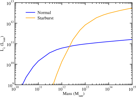
In Figure 1, we plot a comparison of the $L_{\rm c}(M,z)$ relation at $z=1$ for both normal and starburst galaxies. As shown and extracted, based on this simple model, normal galaxies can appear as central galaxies in halo down to smaller mass than the starburst galaxies. In return, starburst galaxies that appear at halo center are brighter at 350 $\mu$m than normal galaxies for the same halo mass if the halo mass is greater than 2.10${}^{12}M_{\sun}$.

For satellites, the normalization $A(M)$ of the satellite CLF can be obtained by defining $L_{\rm s}(M,z)\equiv L_{\rm tot}(M,z)-L_{\rm c}(M,z)$ and requiring that $L_{\rm s}(M,z)=\int_{L_{\rm min}}^{L_{\rm max}}\Phi^{\rm sat}(L|M,z)LdL$, where the minimum luminosity of a satellite is $L_{\rm min}$. In the luminosity ranges of interest, with $\gamma$ between -0.5 to -1, CLFs are mostly independent of the exact value assumed for $L_{\rm min}$ as long as it lies in the range $(10^{6}-10^{8})L_{\sun}$. To describe the total far-IR luminosity of a given dark matter halo we make use of the following phenomenological form:

$$L_{\rm tot}(M,z)=\left\{\begin{array}[]{ll}L_{\rm c}(M,z)&M\leq M_{\rm sat}\\ L_{\rm c}(M,z)\left(\frac{M}{M_{\rm sat}}\right)^{4}&M>M_{\rm sat}\end{array}\right.$$ (9)

Here, $M_{\rm sat}$ denotes the mass-scale at which satellites begin to appear in dark matter halos (taken to $\sim 10^{11}$ for normal galaxies and $5\times 10^{12}$ for starburst galaxies) with luminosities as corresponding to those in the given sample of galaxies. The power-law slope is fixed at 4, independently of the redshift and consistent with total galaxy luminosity-cluster mass relations at near-IR wavelengths (e.g., Lin & Mohr 2004). Whether such a relation holds for far-IR luminosity content of dark matter halos may be testable with Herschel data in the same manner it has been tested at optical and near-IR wavelengths using cluster catalogs.

Since we have divided the far-IR source population into normal and starburst galaxies, we have an additional freedom on how to distribute these galaxies in dark matter halos and this freedom leads to large degeneracies that cannot be simply separated from the luminosity function alone, even if the luminosity function is available for both source types separately. The clustering measurements, including unresolved anisotropies, will make possible to correctly match the mass scales and the relative distribution of normal and starburst populations in dark matter halos in the same manner luminosity functions and clustering studies have been used to identify relative distributions of early- and late-type galaxies (such as the fraction of central galaxies, that appear as late or early type, as a function of the halo mass) at optical wavelengths. If we assume that a fraction of $f_{c}(M,z)$ galaxies at halo centers are normal galaxies and a fraction $f_{s}(M,z)$ of satellite galaxies are normal galaxies, then the luminosity function of normal (n) galaxies can be written as

$$\Phi^{\rm n}(L,z)=\int dM\,\frac{dn}{dM}(z)\,$$ (10)

$$\times \left[f_{c}(M,z)\Phi_{\rm c}^{\rm n}(L|M,z)+f_{s}(M,z)\Phi_{\rm s}^{\rm n}(L|M,z)\right]\,.$$

The luminosity function of starburst galaxies follows by taking $1-f_{c}(M,z)$ and $1-f_{s}(M,z)$ fractions and integrating with CLFs as defined for starburst galaxy population. Given that we have large degeneracies in how to distribute the population, we take the simple approach that in a given halo, we can take the fraction to be same for satellites and centrals (in practice since only one central galaxy is present, this would mean that some halo centers have central galaxies while others have starbursts) and let $f_{c}(M,z)=0.1$, independent of redshift and above the mass at which starburst galaxies appear in halo centers, while this fraction is 1 below the mass scale at which starbursts appear (this mass scale is determined based on a simple match to starburst luminosity functions of Lagache et al. 2003). The exact halo mass and redshift dependences would be some of the interesting parameters that can be potentially extracted from data if adequate statistics are available. The same parameters can be investigated from semi-analytical models of galaxy formation with a focus on the far-IR luminosities and we encourage such studies with existing models.

In Figure 2, we illustrate the comparison between our model, which uses the dark matter halo mass as the starting point to model the galaxy distribution, and Lagache et al. (2003) LFs at 350 $\mu$m at $z=1$, which uses a SED and the 60 $\mu$m LF at low redshifts as a way to build an evolutionary model of source counts with parameters matched to existing data. In Figure 3, we show the normalized redshift distribution of sources (both normal and starburst galaxy types), $\int dz\,n(z)=1$, with fluxes below 100 mJy. As shown here, the redshift distribution is such that the numbers peak at $z>1$, but extends to higher redshifts with a very slow decrease when $z>3$.

While we have not performed a detailed model fit, which we think is premature given the limited data at these far-IR wavelengths, we have varied parameters to get a reasonable consistency between two prescriptions in the literature to model IR source counts. More importantly, our description is outlined in a way that, we think, will allow to extract a model based on future measurements of both luminosity functions and clustering at far-IR wavelengths.

2.2. Far-IR Source Occupation Numbers

By integrating CLFs over luminosity down to a fixed luminosity, we can recover the halo occupation number through

$$\langle N(M)\rangle=\int dL\Phi(L|M)\,.$$ (11)

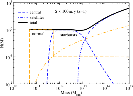
In Figure 4, we illustrate the occupation number at $z=1$ for both normal and starburst populations (and divided to central and satellite galaxies in both cases) with $L_{\rm max}$ corresponding to sources with a maximum flux below 100 mJy at 350 $\mu$m. The combined occupation number cannot be simply described by a power-law though the parameter $\gamma$ describing the satellite CLF luminosity dependence is related to the power-law slope $\beta_{s}$ when occupation number of satellites is described such that $\langle N_{s}(M)\rangle\propto M^{\beta}_{s}$ at the high mass end. Note that the central galaxy occupation number is always one above some mass scale. For sources fainter than 100 mJy at $z=1$ at 350 $\mu$m, the minimum mass at which normal galaxies appear is about few times $10^{10}$ M_☉, while the mass scale at which starburst appear is few times 10¹¹ M_☉. When calculating the power spectrum, we integrate the CLFs over the assumed cut-off luminosity to extract the necessary occupation numbers for both central and satellite galaxies.

While we have provided a bit complicated model, so as to illustrate how the exact modeling can be done once luminosity functions are established at far-IR wavelengths at several different redshifts beyond the low-redshift short wavelength LFs now available from surveys with IRAS, for clustering studies, the behavior of the occupation number as suggested by CLFs can be captured with a model of the form $\langle N_{\rm t}(M,z)\rangle=1+\langle N_{\rm s}(M)\rangle$ when $M>M_{\rm min}(z)$ and 0 otherwise, with the assumption of a central FIRB source in each halo ($\langle N_{\rm c}(M)\rangle=1$) above some mass scale and a power-law distribution of satellites with $\langle N_{\rm s}(M)\rangle=(M/M_{\rm min})^{\beta}$. The value of $M_{\rm min}$, for example, can be readily extracted from occupation numbers shown in Figure 4, or if one needs to vary to a different flux, based on the matching between luminosity and mass from the $L_{c}(M)$ relation shown in Figure 1, for example. Instead of parameters in the CLF, we will show the extent to which we can extract a parameter such as $\beta$ from the 1-halo term of the anisotropy power spectrum given that the small scale clustering is strongly sensitive to the statistics related to satellite galaxies.

Figure 1.— The relation between the 350 $\mu$m luminosity of a central galaxy in a dark matter halo as a function of the halo mass (at a redshift of one). We also show the expected relation between the 350 $\mu$m luminosity of a “normal” galaxy at a redshift of 0.3 as a function of the halo mass. In our modeling, we are assuming that 90% of the central galaxies in halos roughly above 10¹² M_☉ are of the starburst type while at the low mass-end of dark matter halos, all central galaxies are normal galaxy types, in the prescription of Lagache et al. (2003).

Figure 2.— The luminosity function of far-IR sources at $z=1$. In black lines, we show the LFs from the source evolution model of Lagache et al. (2003) subdivided to normal and starburst galaxy populations (thick solid lines). The thin lines are the LFs predicted from the CLF halo model described here, with long dashed lines showing the contribution from central galaxies and the dot-dashed lines showing the contribution from satellites in each of the two types. We obtain a rough agreement between the two different descriptions. With detailed measurements of the LFs with various surveys using Herschel, it is likely that an approach such as the one presented here can be used to establish the underlying source model.

Figure 3.— The predicted normalized redshift distribution for normal and starburst galaxies at 350 $\mu$m, with fluxes less than 100 mJy over all redshifts, based on the CLF halo model presented here.

Figure 4.— The far-IR halo occupation number by integrating CLFs with a maximum luminosity corresponding to a flux of 100 mJy and at for sources at $z=1$. The occupation number is divided to normal and starburst populations and to central (long-dashed lines) and satellite galaxies (dot-dashed lines) in each of the far-IR source types under the classification of Lagache et al. (2003). The thick solid line is the total halo occupation number. The central galaxies of normal type are mostly in low mass halos while central galaxies of starburst type are in halos at the high mass end. The decrease in the central occupation number of starburst galaxies below 1 when $M>10^{13}$ M_☉ is due to the fact that we have only shown the occupation number for sources with fluxes below 100 mJy here.

Figure 5.— Dust removal results for a 10, 400 and 2500 deg² area with Planck and Herschel and for a 2500 deg² area with Planck around the ELAIS-S1 field (from top to bottom and left to right). All spectra are in antenna temperature, $\mu$K${}_{RJ}^{2}$, units at 350 $\mu$m. The foreground and shot-noise residual are respectively the solid red and purple lines. The green solid line is the Galactic dust power spectrum at 350 $\mu$m. The solid light blue and black lines are respectively the combined detector noise (once the optimal frequency mixing is applied) and the combined shot-noise. The FIRB clustering contribution is shown as orange solid, dotted, dashed lines for $\beta$ of 0.85, 0.6, 1 respectively. The blue squares represent the binned theoretical FIRB power spectrum with its error (${\Delta\ell\over\ell}=0.5$).

2.3. Far-IR Source Clustering Bias

In general source clustering at large angular scales can be described with the linear matter power spectrum scaled by a constant, scale-free bias factor such that

$$P_{ss}(k)\approx b^{2}_{s}P^{\rm lin}(k)\,.$$ (12)

In terms of the CLF halo model, this large scale source bias can be written as a combination of the bias of normal and starburst galaxies by noting that the large-scale bias factor of, for example, normal galaxies as a function of source luminosity and the redshift is

$$b^{\rm n}(L,z)=\int dM\,\frac{dn}{dM}(z)\,b_{\rm halo}(M,z)$$ (13)

$$\times \frac{\left[f_{c}(M,z)\Phi_{\rm c}^{\rm n}(L|M,z)+f_{s}(M,z)\Phi_{\rm s}^{\rm n}(L|M,z)\right]}{\Phi^{n}(L,z)}\,.$$

The total galaxy bias, as necessary for unresolved anisotropy clustering measurements, can be calculated by replacing $\Phi(L|M,z)$ with the sum of both normal and starburst CLFs and replacing the LF for normal galaxies with the total.

When separately considered, given that normal galaxies are found mostly in halo centers at the low mass end, the predicted bias factors are generally at the level of $\sim 1$ or slight below one. The starburst galaxies, however, are mostly at halo centers at the high mass end and their bias factors are expected to be larger than 1. Thus, the starburst population is expected to be both strongly clustered and to have both large correlation lengths or bias factors. Using the CLF halo model, if the clustering spectrum of resolved sources at $z\sim 1$ with fluxes above 100 mJy is measured, we find that the bias factors will be expected to be order 2.0. Such a large bias factor, or equivalently a large correlation length, is consistent with some of the limited suggestions in the literature that far-IR sources with bright fluxes are strongly clustered (e.g., Blain et al. 2004). At the same flux cut, the unresolved anisotropies are expected to have a bias factor of the order 1.1. This value is substantially below the bias factor of resolved sources at the same flux cut since unresolved anisotropies are dominated by sources that are substantially fainter than the sources just below the flux cut.

2.4. Shot-noise power spectrum

In addition to the clustering signal, at small angular scales, the finite density of sources leads to a shot-noise type power spectrum in the IRB spatial fluctuations. This shot-noise can be estimated through number counts such that $C_{l}^{\rm shot}=\int_{0}^{S_{\rm cut}}dS\,S^{2}(dN/dS)$ when $S_{\rm cut}$ is the flux cut off value related to the removal of resolved sources.We use the confusion noise as estimated by Hspot for Herschel, 25, 29, 24.5 mJy (5$\sigma$) at 250, 350 and 500 $\mu$m and by Negrello et al. (2004) for Planck, 29.2, 115, 323 and 705 mJy (5$\sigma$) at 217, 353, 545 and 857 GHz.

3. Foreground Separation

We model the Galactic dust with the model 8 (two temperature model) of Finkbeiner et al. (1999) and maps from Schlegel et al. (1998) (cleaned IRAS with a calibration obtained on DIRBE with an effective angular resolution of 6 arcminutes) over the frequency range of 217 GHz to 1200 GHz (250 $\mu$m to 1.2 mm). We fit with a power law the power spectrum of the Galactic dust of a 4900 deg² area around ELAIS-S1 field at each frequency. We use the variance of the signal in our smaller fields to scale down the fitted power spectrum to these smaller fields. The FIRB anisotropy power spectrum modeled at 350 $\mu$m following the halo model above is interpolated to other wavelengths using the mean spectrum from COBE/FIRAS (Fixsen et al. 1998) as

$$I_{\nu}=\tau_{0}(\nu/\nu_{0})^{\alpha}B_{v}(T)\ ,$$ (14)

with $\tau_{0}=(1.3\pm 0.4)\times 10^{-5}$, $T=18.5\pm 1.2$K and $\alpha=0.64\pm 0.12$.

To study the extent to which foreground dust confusion can be reduced we used the cleaning technique outlined in Tegmark et al. (2003), where multifrequency maps from WMAP first-year data were used to produce the so-called TOH foreground-cleaned CMB map. The technique recommends taking a linear combination of observed $a_{\ell m}$’s in each frequency band $i$, $a_{\ell m}=\sum_{freq=i}w^{i}_{\ell}a^{i}_{\ell m}$, with weights $w_{i}$ chosen to minimize foreground contamination from Galactic dust. We decompose the signal at each frequency as $a^{i}_{\ell m}=u^{i}_{\ell m}+f^{i}_{\ell m}+n^{i}_{\ell m}$ where $u$, $f$, and $n$ stand respectively for unresolved FIRB, foregrounds (CMB and Galactic dust), and noise. We then minimize the resulting power spectrum of extragalactic FIRB fluctuations, assuming the frequency spectrum of this component follows that of Fixsen et al. (1998) through $\langle|a_{\ell m}|^{2}\rangle={\bf w_{\ell}}^{T}{\cal C}{\bf w_{\ell}}$ using weights under the constraint $w_{\ell}^{T}\cdot{\bf e}=1$, where ${\bf e}$ is a column vector with the relative amplitude of the FIRB spectrum.

The above condition allows to sum the different frequencies without reducing the FIRB component, and permits to optimally subtract the Galactic dust (CMB itself as a foreground only makes a minor impact at frequencies above 500 GHz). Here, the ${\cal C}^{ij}_{\ell}$ matrix represents $\langle(a^{i}_{\ell m})^{\dagger}a^{j}_{\ell m}\rangle$. As derived in Tegmark et al. (2003), the weights that minimize the power $\langle|a_{\ell m}|^{2}\rangle$ are

$${\bf w_{\ell}}=\frac{{\cal C}^{-1}{\bf e}}{e^{T}{\cal C}^{-1}e}\,.$$ (15)

The estimate of residual dust level with this method is clearly optimistic since the FIRB spectrum is poorly known. We will quantify the impact of the uncertainty related to the spectrum in terms of an overall uncertainty in the cumulative signal-to-noise ratio for detection of FIRB fluctuations in the presence of Galactic dust. To quantify our results, we center our simulation around ELAIS-S1 (RA-DEC : 7.8,-44.2), which is a preferred region known to be least contaminated with cirrus even after considering a large region around this field.

In our calculations we assume an uncorrelated noise power spectrum, with $\langle n_{\ell m}^{i}n_{\ell^{\prime}m^{\prime}}^{j}\rangle=\delta_{ij}\delta_{mm^{\prime}}\delta_{\ell\ell^{\prime}}N_{\ell}^{\prime}$, between SPIRE bands. For $N_{l}^{\prime}$, we take 1$\sigma$ noise levels for a SPIRE 10 deg² survey with a 1000 hour integration: 1.6, 2.1 and 1.7 mJy at 250, 350, 500 $\mu$m (obtained from HSpot) and then degrade as the survey area is increased. To combine Herschel data with Planck, we make use of 217, 353, 545 and 857 GHz channels of Planck HFI with equivalent noise of 13.4, 25.2, 48.4 and 55.4 mJy . Since wide-field Herschel-SPIRE maps are raster-scanned, 1/f-noise impact measurements of large angular scale fluctuations. We model this by modifying the overall noise spectrum to be $N_{\ell}=N^{\prime}_{\ell}(1+\ell_{\rm knee}/\ell)$ (e.g., Crawford 2007) and take $\ell_{\rm knee}=10^{3}$ corresponding to a 1/f knee at a frequency of 100 mHz with a scan rate of 60”/sec. While we include 1/f-noise, to effectively remove it requires two passes of the same field in orthogonal directions. Generally, this requires that for a given area, one spend twice as long than when a survey is conducted for point source detections only. Given the maximum scan rate, for a fixed integration time, there is also a maximum area one can cover, but we have ignored this restriction here when estimating the signal-to-noise ratio as a function of the sky area as the maximum scan rate is not yet established. We neglect Planck 1/f-noise residual, since we believe it would not be as strong as Herschel one on our scales of interest due to Planck’s faster scanning speed.

Figure 6.— Total signal-to-noise on the estimate of the FIRB clustering power spectrum. We took into account the instrumental noise, the cosmic variance, and the foreground and shot-noise residuals for different sky coverage (from 3 to 5000 deg²). The blue triangles and red squares represent a “clean” area selected from SFD98 dust map and centered around ELAIS-S1 field using Herschel and Herschel+Planck, respectively. In each selected survey size, we assume a total integration time of 1000 hours with Herschel-SPIRE, while the integration time for Planck is independent of the survey area given that Planck data is an all-sky survey be design. The solid orange area represents the signal-to-noise ratio achievable when FIRB spectrum is taken to be uncertain at the $\pm$ 1 $\sigma$ level of Fixsen et al. (1998) analytical model (see, Eq. 3).

4. Results & Discussion

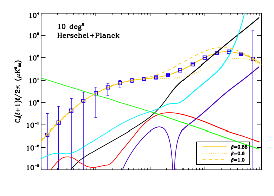
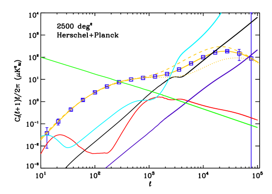
Figure  5 shows examples of the FIRB power spectrum estimated on a 10, 400, and 2500 square degree fields around a very low foreground Galactic dust field centered around ELAIS-S1 using the 3 SPIRE bands (corresponding to central frequencies of 577, 833 and 1200 GHz) with a 1000 hours integration time and 4 of Planck frequency bands (217, 353, 545, 857 GHz, assuming the 14 month survey). According to figure  5, these surveys can measure accurately the power spectrum of FIRB on scales smaller than 30 arcminutes ($\ell\simeq 400$), however, the smallest scales might be biased by the confusion noise coming from the shot-noise term. Larger scales are not very well measured by the 10 deg² survey due to a large remaining cosmic variance. On the other hand, the Galactic dust residuals are much smaller for the smaller area survey (typically a factor 5 to 10 in power).

4.1. Optimal survey area

In addition to 3 field sizes highlighted in Fig. 5, it could be that the angular power spectrum might be measured at a more significant level if the field size is optimized for these measurements given a finite integration time. We therefore compute the noise level and the Galactic dust level in the FIRB power spectrum estimate for different field size assuming a total of 1000 hour integration time for Herschel/SPIRE observations. To show quantitatively how well different field sizes are measuring clustering of the unresolved component, we computed the total signal to noise (optimal sum on all the mode $\ell$), with the signal $C^{\rm clus}_{\ell}$ being the FIRB power spectrum due to clustering, and the noise being the sum of the instrumental noise ($N_{\ell}$) variance, the cosmic variance and the residual Galactic dust and shot-noise :

$$S/N=\sqrt{\sum_{\ell=\ell_{min}}^{\ell_{max}}\left({C^{\rm clus}_{\ell}\over X_{\ell}}\right)^{2}}\,,$$ (16)

where

$$X_{\ell}=(N_{\ell}+C^{\rm FIRB}_{\ell})\sqrt{2\over(2\ell+1)f_{\rm sky}}+R_{\ell}\,,$$ (17)

and $C^{\rm FIRB}_{\ell}=C^{\rm clus}_{\ell}+C_{\ell}^{\rm shot}$ and $f_{\rm sky}$ is the fraction of sky covered. The residual shot-noise is taken as the combination of the 1 $\sigma$ uncertainties computed by a Fisher matrix analysis (Tegmark et al. 1997) at each frequency for each instrument (Planck and Herschel/SPIRE), given a model where dust and FIRB clustering power spectrum shape are known. These residual shot-noise estimates are probably optimistic, especially for Planck since its angular resolution does not allow to measure the small angular scale ($\theta<0.5^{\prime}$) where the shot-noise term dominates.

Figure 7.— The signal-to-noise ratio on the estimate of the FIRB clustering power spectrum as a function of the multipole. Top: The signal-to-noise as a function of the multipole. Bottom: The cumulative signal-to-noise ratio as a function of the multipole. As illustrated, Planck (HFI) can make higher signal-to-noise clustering measurements of FIRB anisotropies, though the measurements are limited to multipoles of less than about 4000. The combination of Herschel and Planck over 400 deg², with Herschel imaging data in an integration of 1000 hours, has the highest overall signal-to-noise ratio for the clustering measurements.

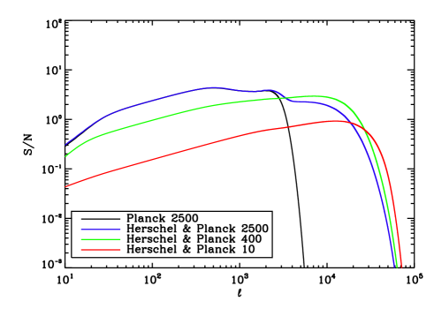
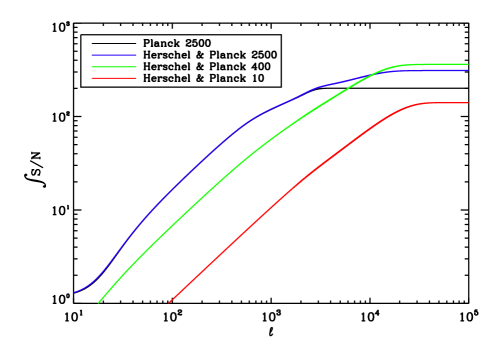
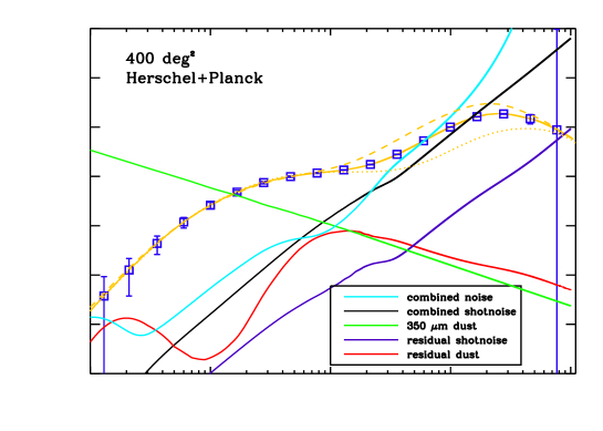
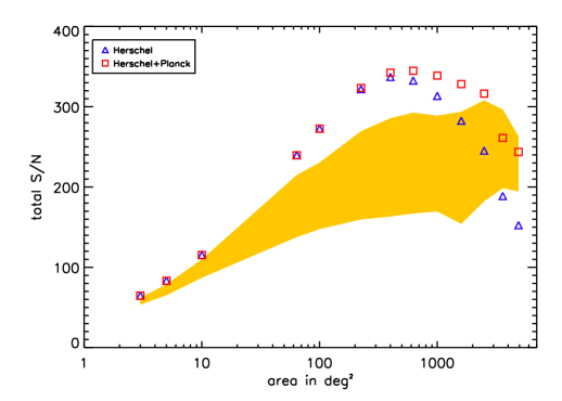
The results obtained are summarized in Figure 6. The signal-to-noise ratio increases with the area covered from 65 with 3 deg² to 360 with 400-600 deg² due to the decrease of the cosmic variance, and then decreases due to the increase of the Galactic dust residual and the lower observation depth. Adding the Planck channels at 217, 353, 545 and 857 GHz does not change the overall sensitivity if the used Planck field is smaller than 400 deg², but they increase substantially the sensitivity for field of larger size. Figure 7 shows that Planck sensitivity dominates at large scale ($\ell<3000$) for field above 2500 deg², but that a smaller Herschel field around 400 $deg^{2}$ is more optimal at measuring smaller scale ($\ell>3000$), whereas fields of few tens square degree lose a lot of sensitivity in the clustering part ($1000<\ell<10000$) of the FIRB power spectrum due to the cosmic variance. The “optimal” area (400 deg²) corresponds to an observation depth of about 51, 66, and 54 mJy (5 $\sigma$, only instrumental) at 250, 350, 500 $\mu$m, we believe this “optimal” depth to be robust to a change in integration time, given our shot-noise level estimates.

As discussed in Section 3, to estimate the confusion associated with Galactic dust due to the uncertain extragalactic FIRB spectrum, we vary the spectrum based on uncertainties in Fixsen et al. (1998) spectrum from COBE/FIRAS by drawing 100 simulations assuming uncertainties in the parameters describing the spectrum are Gaussian distributed (see, Eq. 3). Again, we separate the Galactic dust from the FIRB and compute the total signal-to-noise ratio. Figure 6 (orange area) shows that the sensitivity to the clustering is degraded by 10% to 35% on average and that the uncertainty on the FIRB spectrum generates a 10% to 30% uncertainty on the total sensitivity. Even with these uncertainties, the 400 deg² survey remains more sensitive than the few ten square degree surveys. While uncertainties in foreground emission largely impacts the overall signal-to-noise ratio for a detection of FIRB anisotropy spectrum, an anisotropy study in a 400 deg.² field is still important given the limited knowledge we have on the unresolved component that accounts for up to 90% of the background light at 350 $\mu$m.

Figure 8.— Constraints on $\beta_{s}$ and the source bias factor from unresolved FIRB clustering measurements with Herschel-SPIRE and Planck. The ellipse describe the 95% confidence level errors after marginalizing over 2 additional parameters related to the uncertain redshift distribution of sources. As shown, Planck measurements (over 2500 deg²) alone do not establish information captured in the 1-halo term, such as the satellite occupation number, while with Herschel, small angular scale clustering is adequately measured to properly establish statistics related to far-IR sources, such as the slope of the occupation number. While we have only considered clustering of unresolved anisotropies here, in a large-are survey, the combination of LFs, resolved source clustering, and unresolved anisotropies can be used to establish an improved model with parameterization based on the CLFs.

4.2. Astrophysical Information in Unresolved Anisotropies

To study the extent to which these anisotropy measurements can be used for astrophysical studies, we considered extraction of halo model parameters. For this, we assume a fiducial model for the source distribution and allow variations in certain parameters related to this model to study how the likelihood changes. This is done by constructing the Fisher matrix,

$${\bf F}_{ij}=-\left<\partial^{2}\ln L\over\partial p_{i}\partial p_{j}\right>_{\bf X}\,,$$ (18)

where $L$ is the likelihood of observing a data set ${\bf X}$ given the true parameters $p_{1}\ldots p_{n}$. Since the variance of an unbiased estimator of any parameter $p_{i}$ cannot be less than the Cramer-Rao bound captured by $({\bf F}^{-1})_{ii}$, the Fisher matrix quantifies the best statistical errors on parameters possible with a given data set (Tegmark et al. 1997). We refer the reader to Knox et al. (2001) for a prior application of the Fisher matrix to study how well far-IR background anisotropies can be used to establish properties of the source distribution.

For the clustering of unresolved anisotropies, the Fisher matrix becomes

$${\bf F}_{ij}=\sum_{\ell=\ell_{\rm min}}^{\ell_{\rm max}}\frac{1}{X_{\ell}^{2}}{\partial C_{\ell}^{\rm clus}\over\partial p_{i}}{\partial C_{\ell}^{\rm clus}\over\partial p_{j}}\,,$$ (19)

where $X_{\ell}$ follows from Equation 17. To establish the relative importance of Herschel given Planck high frequency observations and to get an order-of-magnitude estimate on how well unresolved anisotropies can be used to extract some information on the underlying source distribution, we consider a model with four parameters involving large-scale bias factor, small scale occupation number captured by the power-law slope $\beta_{s}$, and two parameters to describe the redshift distribution of unresolved sources with fluxes fainter than the point source detection. Motivated by the redshift distribution predicted by the CLF halo model and shown in Fig. 3, we parameterize the redshift distribution with a quadratic function that is zero at $z=0$. We calculate the Fisher matrix by varying these four parameters and marginalize over the uncertain redshift distribution by projecting the 4-dimensional Fisher matrix to two dimensions involving bias and the power-law slope of the occupation number.

In Figure 8, we show the expected 95% confidence level errors on the slope parameter $\beta_{s}$ on the halo occupation number and the overall bias factor describing the large angular scale clustering. To recover the occupation number in detail, clustering measurements at smaller angular scales are required to probe the 1-halo part and this is not possible with, for example, Planck high frequency data alone. As shown in Fig. 5, the required measurements can be easily achieved with Herschel-SPIRE since Planck channels do not have the adequate resolution. Furthermore, the combination of Planck and Herschel over 2500 deg.² allows estimates of the occupation numbers and the bias factor at the level of a few percent at the 95% confidence level even after accounting for the uncertain redshift distribution of sources below the point source detection level. For smaller area surveys down to the same depth, there is a general degradation on parameter determination with the factor $\sqrt{f_{\rm sky}}$.

In practice, once anisotropy measurements become available, clustering analyses can be improved by combining unresolved fluctuations with information from the clustering of resolved sources, number counts, and luminosity functions. The mechanisms to carry out such studies already exist (See example involving 3.6$\mu$m Spitzer data in Sullivan et al. 2007), but what is now clearly needed is a survey of required area and sensitivity. Here we have shown that a survey of order 10³ deg.² provides maximal information on the clustering of unresolved fluctuations.

Finally, it may also be possible to use these anisotropy maps for a weak lensing analysis in the same manner CMB maps are now proposed for lensing studies given the large magnification bias at far-IR wavelengths (e.g., Blain 1998). The same maps can also be extended to cross-correlate with Planck temperature anisotropy data at low frequencies and at large angular scales to detect the integrated Sachs-Wolfe (ISW) effect and at small angular scales to detect the CMB lensing-far IR source cross-correlation. The latter lensing-source cross-correlation has been detected with WMAP and NVSS radio survey at the 2$\sigma$ confidence level (Smith et al. 2007), but when Planck data are combined with a wide-survey of Herschel of order 1000 deg², the cross-correlation can be detected at $>$ 20 $\sigma$ confidence level (Song et al. 2003). Once a better understanding 1/f-noise etc become available, it may be useful to returns to these topics to exploit the full information content of Herschel.

5. Summary

Below the point source detection limit in upcoming far-IR surveys with Planck and Herschel-SPIRE, correlations in the large-scale structure will lead to clustered anisotropies in the unresolved component of the far-infrared background (FIRB). The angular power spectrum of the FIRB anisotropies could be measured in these surveys and will be one of the few limited avenues to study some, though limited, information on the faint sources that dominate the background light at these wavelengths.

To study the statistical properties of these anisotropies, the confusion from foreground Galactic dust emission needs to be reduced even in the “cleanest” regions of the sky. The multi-frequency coverage of Planck and Herschel-SPIRE instrument allows the foreground dust to be partly separated from the extragalactic background composed of dusty starforming galaxies as well as faint normal galaxies. The separation improves for fields with sizes greater than a few hundred square degrees and when combined with Planck data. Here, we have shown that an area of about $\sim$ 400 degrees² observed for about 1000 hours with Herschel-SPIRE and complemented by Planck provides maximal information on the anisotropy power spectrum.

Assuming such a survey will be conducted, we have discussed the scientific studies that can be done with measurements of the unresolved FIRB anisotropies including a few percent accurate determination of the large scale bias and the small-scale halo occupation distribution of FIRB sources with fluxes below the point-source detection level. In practice, in addition to the clustering spectrum of unresolved anisotropies, measurements such as the luminosity function and the correlation function of resolved sources as well as their redshift distribution must be modeled within the same framework. Here, we have provided a detailed outline of such a strategy based on the conditional luminosity functions associated with the halo approach to large-scale structure.

Acknowledgments:

We thank SPIRE SAG-1 and Open-Time Key Projects groups for useful discussions. We thank G. Lagache and her collaborators for making results of their source modeling publicly available in electronic form. This work was supported at UC Irvine by a McCue Fellowship (to AA), NSF CAREER AST-0645427, and NASA support for science studies with Herschel-SPIRE Guaranteed Time Observations at UC Irvine with JPL Contract 1295096).

References

- (1) Berlind, A. A., Weinberg, D. H., Benson, A. J. et al. 2003, ApJ, 593, 1
- Blain (1998) Blain, A. W. 1998, MNRAS, 295, 92
- (3) Blain, A. W., Smail, I., Ivison, R. J., Kneib, J.-P. & Frayer, D. T., 2002, Phys. Rept. 369, 111
- (4) Blain, A. W., Chapman, S. S., Smail, I. & Ivison, R. J. 2004, ApJ, 611, 725
- (5) Cooray, A., & Milosavljević, M. 2005, ApJ, 627, L89
- (6) Cooray, A. 2005, MNRAS, 365, 842
- Cooray & Sheth (2002) Cooray, A. & Sheth, R. 2002, Physics Reports, 372, 1 (astro-ph/0206508)
- Crawford (2007) Crawford, T. 2007, astro-ph/0702608
- Dwek et al. (1998) Dwek, E., et al. 1998, ApJ, 508, 106
- Griffin et al. (2006) Griffin, M. et al. 2006, in “Studying Galaxy Evolution with Spitzer and Herschel”, Crete (astro-ph/0609830)
- Finkbeiner et al. (1999) Finkbeiner, D.P., Davis, M. & Schlegel, D.J. 1999, ApJ, 524, 867
- Fixsen et al. (1998) Fixsen, D.J., Dwek, E., Mather, J.C., Bennett, C.L. & Shafer, R.A. 1998, ApJ, 508, 123
- Haiman & Knox (2000) Haiman, Z. & Knox, L. 2000, ApJ, 530, 124
- Hauser & Dwek (2001) Hauser, M. & Dwek, E. 2001, ARAA, 39, 249
- Knox et al. (2001) Knox, L., Cooray, A., Eisenstein, D. & Haiman, Z. 2001, ApJ, 550, 7
- (16) Kravtsov, A. V., Berlind, A. A., Wechsler, R. H., Klypin, A. A., Gottlöber, S., Allgood, B., & Primack, J. R. 2004, ApJ, 609, 35
- Lagache et al. (2003) Lagache, G., Dole, H. & Puget, J.-L. 2003, MNRAS, 338, 555
- Lagache et al. (2005) Lagache, G., Puget, J.-L., Dole, H. 2005, ARA&A, 43, 727
- (19) Limber, D. 1954, ApJ, 119, 655
- Lin & Mohr (2004) Lin, Y.-T. & Mohr, J. J. 2004, ApJ, 617, L879
- Negrello et al. (2007) Negrello, M. et al. 2007, astro-ph/0703210
- Puget et al. (1996) Puget, J. L. et al. 1996, A&A, 308, L5
- Schlegel et al. (1998) Schlegel, D.J., Finkbeiner, D.P. & Davis, M. 1998, ApJ, 500, 525
- Scott & White (1999) Scott, D. & White, M. 1999, A&A, 346, 1
- Smith et al (2007) Smith, K. M., Zahn, O. & Doré, O. 2007, arXiv:0705.3980
- Song et al (2003) Song, Y.-S., Cooray, A., Knox, L. & Zaldarriaga, M. 2003, ApJ, 590, 664
- Sullivan et al. (2007) Sullivan, I. et al. 2007, ApJ, 657, 37 (astro-ph/0609451)
- Tegmark et al. (2003) Tegmark, M., de Oliveira-Costa, A. & Hamilton, A. 2003, Phys. Rev. D, 68, 123523
- Tegmark et al. (1997) Tegmark, M., Taylor, A. & Heavens, A. 1997, ApJ, 480, 22
- (30) Vale, A., & Ostriker, J. P. 2004, MNRAS, 353, 189
- (31) Yang, X., Mo, H. J., & van den Bosch, F. C. 2003, MNRAS, 339, 1057
- (32) Yang, X., Mo, H. J., Jing, Y. P., & van den Bosch, F. C. 2005, MNRAS, 358, 217