Compressible Turbulence in Galaxy Clusters: Physics and Stochastic Particle Re-acceleration

Abstract

We attempt to explain the non-thermal emission arising from galaxy clusters as a result of the re–acceleration of electrons by compressible turbulence induced by cluster mergers. On the basis of the available observational facts we put forward a simplified model of turbulence in clusters of galaxies focusing our attention on the compressible motions. In our model intracluster medium (ICM) is represented by a high beta plasma in which turbulent motions are driven at large scales. The corresponding injection velocities are higher than the Alfvén velocity. As a result, the turbulence is approximately isotropic up to the scale at which the turbulent velocity gets comparable with the Alfvén velocity. These motions are most important for the energetic particle acceleration, but at the same time they are subjected to most of the plasma damping. Under the hypothesis that turbulence in the ICM is highly super– Alfvénic the magnetic field is passively advected and the field lines are bended on scales smaller than that of the classical, unmagnetized, ion–ion mean free path. This affects ion diffusion and the strength of the effective viscosity. Under these conditions the bulk of turbulence in hot (5–10 keV temperature) galaxy clusters is likely to be dissipated at collisionless scales via resonant coupling with thermal and fast particles. We use collisionless physics to derive the amplitude of the different components of the energy of the compressible modes, and review and extend the treatment of plasma damping in the ICM. We calculate the acceleration of both protons and electrons taking into account both Transit Time Damping acceleration and non-resonant acceleration by large scale compressions. We find that relativistic electrons can be re–accelerated in the ICM up to energies of several GeV provided that the rms velocity of the compressible turbulent–eddies is $(V_{L}/c_{s})^{2}\approx 0.15-0.3$; $c_{s}$ is the sound speed in the ICM. We find that under typical conditions $\approx$ 2–5 % of the energy flux of the cascading of compressible motions injected at large scales goes into the acceleration of fast particles and that this may explain the observed non–thermal emission from merging galaxy clusters.

1 Introduction

In the last years observations of galaxy clusters have shown that non–thermal components are mixed together with the thermal component of the intracluster medium (ICM). A fraction of massive galaxy clusters hosts diffuse radio emission in the form of radio halos, Mpc–sized diffuse synchrotron radio sources at the cluster center, and radio relics, elongated diffuse synchrotron radio sources at the cluster periphery. This directly proves the presence of GeV relativistic electrons (and/or positrons) and of $\mu$G magnetic fields diffused on Mpc scales through the cluster volume (e.g., Feretti 2005, for a review). A related issue is the discovery of non–thermal emission in the hard X–ray band detected in a few galaxy clusters (e.g., Fusco–Femiano et al. 2004; Rephaeli, Gruber, Arieli  2006).

The most spectacular example of non–thermal emission from galaxy clusters is that of giant radio halos. These are very extended (Mpc) synchrotron radio emissions, not connected with cluster radio sources, at the center of clusters, with a steep spectrum and a typical synchrotron luminosity in the range $\approx 10^{40}-10^{42}$erg s^-1. A remarkable point is that the emitting particles have a life–time considerably shorther than that necessary to diffuse over the scales of these radio halos, and this poses a theoretical problem on their origin (e.g., Jaffe 1977). In principle if the content of cosmic ray hadrons in the ICM is sufficiently large, fast electrons and positrons may be continuously injected in the ICM via hadronic collisions between cosmic–rays and thermal protons (Dennison 1980; Blasi & Colafrancesco 1999), alternatively different forms of in situ–stochastic acceleration and re–acceleration operating for a small fraction of the cluster life may provide a viable source for high energy emitting particles (Schlickeiser et al. 1987; Brunetti et al. 2001; Petrosian 2001). Future gamma ray observations (GLAST, Cerenkov telescopes) will constrain the content of cosmic–ray hadrons in galaxy clusters and provide an important tool to better understand the origin of the relativistic particles in the ICM (e.g. Reimer 2004 & Blasi et al. 2007 for recent reviews).

It is believed by several authors that the re–acceleration scenario may provide a promising picture to explain the bulk of present–day radio data (e.g., reviews by: Brunetti 2003,04; Petrosian 2003; Blasi 2004; Hwang 2004; Feretti 2005). This model essentially relies on the hypothesis that a fraction of the kinetic energy associated with cluster–cluster mergers is channelled into turbulence and re–acceleration of relativistic particles in the ICM.

MHD turbulence is known to be an important agent for particle acceleration since Fermi (1949) first pointed this out. Second order Fermi acceleration by MHD turbulence was appealed for acceleration of particles in many astrophysical environments, e.g. Solar wind, Solar flares, ICM, gamma-ray bursts (see Schlickeiser & Miller 1998; Chandran 2003; Brunetti et al. 2004; Petrosian & Liu 2004; Cho & Lazarian 2006; Petrosian et al. 2006; Becker, Le & Dermer 2006; Dogiel et al. 2007). Naturally, properties of compressible MHD turbulence (see Shebalin, Matthaeus, & Montgomery 1983; Higdon 1984; Montgomery, Brown, & Matthaeus 1987; Shebalin & Montgomery 1988, Zank & Matthaeus 1992; Cho & Lazarian 2003 and references therein) are essential for understanding the acceleration mechanisms.

Among the advances in understanding MHD turbulence, we would like to mention the Goldreich & Sridhar (1995; henceforth GS95) model of turbulence. GS95 dealt with incompressible MHD turbulence and showed that Alfvén and pseudo-Alfvén modes follow the scale-dependent anisotropy of $l_{\|}\sim l_{\perp}^{2/3}$, where $l_{\|}$ is the size of the eddy along the local mean magnetic field and $l_{\perp}$ that of the eddy perpendicular to it. Lithwick & Goldreich (2001) conjectured that this scaling of incompressible modes is also true for Alfvén modes and slow modes in the presence of compressibility. In Cho & Lazarian (2002; 2003, henceforth CL03) the rational for considering separately the evolution of slow, fast and Alfvén mode cascades was justified. The numerical simulations in CL03 and Kowal & Lazarian (2006) verified that Alfvén and slow mode velocity fluctuations are indeed consistent with the GS95 scaling, while fast modes exhibit isotropy in both gas-pressure (high $\beta_{pl}$) and magnetic-pressure (low $\beta_{pl}$) dominated plasmas. The former case is the most appropriate for clusters of galaxies that we deal in this paper.

A single most important change in the paradigm that has become obvious recently is that if the turbulent–energy injection happens at large scales, the cascading Alfvénic mode is presented at sufficiently small scales by very elongated eddies. Thus the interactions of these mode with cosmic rays differs considerably from that of the isotropic eddies that earlier researchers dealt with. Under these conditions nearly isotropic fast modes were identified as the dominant agent for scattering and resonance acceleration (Yan & Lazarian 2002). As a consequence of this, our understanding of energetic particle-turbulence interactions via gyroresonance and the Transit-Time Damping (TTD) (Chandran 2000; Yan & Lazarian 2002, 2004; Farmer & Goldreich 2004; Cassano & Brunetti 2005) as well as the non-resonance acceleration of cosmic rays by large scale compressible motions (see Ptuskin 1988, Chandran 2003, Cho & Lazarian 2006) has been altered. This calls for the corresponding advances in the treatment of cosmic–ray acceleration in the environment of clusters of galaxies (see e.g. Brunetti 2006 & Lazarian 2006a).

2 Outline of the paper

In this paper we proceed in three main steps :

I) As a first point we discuss the problem of turbulence in the ICM and work up a simplified but physical picture of the properties and relevant scales of turbulence in galaxy clusters. As we discuss below (see §3.1) the plasma in clusters of galaxies is expected to be both magnetized and turbulent. Its Reynolds numbers are expected to vary as the magnetic field grow (§3.2), but they are expected to be high enough to allow turbulence to be excited. Finally turbulence in hot galaxy clusters is expected to be dissipated via collisionless dampings and this makes the particle acceleration process a natural consequence (§3.4). This part of the paper is mainly designed to provide a reference picture for observers and a viable astrophysical starting point for theoretical developments.

II) As a second point we discuss the physics of compressible motions in the collisionless regime. This part of the paper is a necessary extension of previous seminal studies of collisionless turbulence and is aimed at the presentation of necessary general equations to use in the paper. In particular to characterize the plasma-cosmic rays interactions we characterize the compressible motions using dielectric tensor (§4.1), give the expression for the energy spectrum of the fast modes in §4.2 and describe the TTD damping in intracluster plasma in §4.3; complex expressions and calculations are reported in Appendices A–C .

III) Finally we discuss the issue of stochastic particle acceleration in galaxy clusters by compressible turbulence. The resonant TTD acceleration is discussed in §5.1, while the effect of non-resonant acceleration is discussed in §5.2. In §6 we discuss the results in the framework of the particle re–acceleration model in galaxy clusters: in §6.1 we briefly review the basic physics of cosmic rays in galaxy clusters, and in §6.2 we present detailed calculations on particle re–acceleration in the ICM. Here we claim that compressible turbulence may drive efficient particle acceleration in the ICM. This is an extension of recent studies on the argument and provides a view of the process of particle re–acceleration in the ICM which is additional (or alternative) to that of Alfvénic acceleration.

In §7 we discuss the most relevant findings and simplifications, and in §8 we provide a short summary.

3 Turbulence in the ICM

3.1 Injection of turbulence in the ICM

Cluster mergers and accretion of matter at the virial radius may induce large–scale motions with $V_{L}\sim 1000$ km s^-1 in massive clusters. Numerical simulations suggest that turbulent motions may store an appreciable fraction, 5–30%, of the thermal energy of the ICM (e.g., Sunyaev, Bryan & Norman 2003; Dolag et al. 2005; Vazza et al. 2006). Simulations of merging clusters provide an insight into the gas dynamics during a merger event (e.g., Roettiger, Burns, Loken 1996; Roettiger, Loken, Burns 1997; Ricker & Sarazin 2001): sub–clusters generate laminar bulk flows through the sweeped volume of the main clusters which inject turbulence via e.g. Kelvin–Helmholtz instabilities at the interface of the bulk flows and the primary cluster gas. The largest turbulent eddies decay into smaller and turbulent velocity fields developing a turbulent cascade.

A simple, but well motivated by physical arguments, semi–analytical approach allows to follow the cosmological injection of merger–turbulence. Calculations from Cassano & Brunetti (2005) suggest that turbulence in the ICM is transient being mostly injected during the most massive mergers. However, since more frequent minor mergers may also contribute to the injection of such turbulence, some minimum level of turbulence should be rather ubiquitous in the ICM. In these calculations turbulence is assumed to be injected in the cluster volume swept by the sub-clusters, which is bound by the effect of the ram pressure stripping, and the turbulent energy is calculated as a fraction of the ${\rm PdV}$ work done by the sub-clusters infalling onto the main cluster. Essentially merger–driven turbulence is powered by the gravitational potential well and thus the energy of this turbulence should approximatively scale with the cluster thermal energy (Cassano & Brunetti 2005). Support to this scaling comes from a recent analysis of a sample of galaxy clusters from cosmological numerical simulations (Vazza et al. 2006).

Turbulence is an important ingredient in the physics of the ICM as it is necessary to understand the amplification of magnetic fields in clusters (Dolag et al. 2002; Schekochihin et al. 2005; Subramanian et al. 2006), an issue closely related to the non–thermal emission from clusters but that we will not address in this paper. Turbulence might provide a source of heating to balance the cooling of cluster cores (Fujita, Matsumoto & Wada 2004), and the knowledge of the basic aspects of turbulence in galaxy clusters is also crucial to model the transport of heat and metals in the ICM (Narayan & Medvedev 2001; Cho et al., 2003; Voigt & Fabian 2004; Lazarian 2006b).

In spite of obvious observational challenges, indications of some level (at least 10–20% of the thermal energy) of turbulence in the ICM comes from gas–pressure maps in the X–rays (Schuecker et al. 2004), and also from the lack of resonant scattering from X–ray spectra (Churazov et al. 2004; Gastaldello & Molendi 2004).

Interestingly enough, also upper limits to the turbulent–energy content in the ICM were obtained in a few nearby galaxy clusters from kinematical arguments related to the properties of H$\alpha$ and X–ray filaments (e.g. Fabian et al. 2003; Crawford et al. 2005; Sun et al. 2006). Assuming that turbulence is driven at hundred–kpc scales the above upper limits actually can be used to place upper limits on the intensity of strong turbulence in the ICM (supersonic or trans–sonic turbulence).

3.2 Reynolds Number and developing of turbulence in the ICM

In this Section we discuss the important issue of the Reynolds number of the fluid in the ICM, and derive its value by assuming a simple, but physically motivated, scenario.

A fluid becomes turbulent when the rate of viscous dissipation at the injection scale, $L_{o}$, is much smaller than the energy transfer rate, i.e. when the Reynolds number is ${\it Re}=V_{L}L_{o}/\nu_{K}\gg 1$, where $V_{L}$ is the injection velocity and $\nu_{K}$ is the kinetic fluid viscosity. The main source of uncertainty here comes from our ignorance of $\nu_{K}$ in the ICM.

If the ICM were not magnetized $\nu_{K}\sim l_{mfp}v_{i}/3$, were $v_{i}$ is the velocity of thermal ions, and $l_{mfp}$ is the ion–ion mean free path in case of pure Coulomb interactions (e.g., Braginskii 1965):

$$l_{mfp}\sim 15000\,\left({{n_{e}}\over{10^{-3}{\rm cm}^{-3}}}\right)^{-1}\left({{T}\over{\rm 8\,keV}}\right)^{2}\left({{40}\over{\ln\Lambda}}\right)\,\,\,\,\,\,(\rm pc)$$ (1)

where $\ln\Lambda$ is the Coulomb logarithm.

Thus the corresponding Reynolds number would be:

$${\it R}e\sim 52\,\Big{(}{{V_{L}}\over{1000\,{\rm km/s}}}\Big{)}\Big{(}{{L_{o}}\over{300\,{\rm kpc}}}\Big{)}\Big{(}{{n_{\rm th}}\over{10^{-3}{\rm cm}^{-3}}}\Big{)}\Big{(}{{T}\over{\rm 8\,keV}}\Big{)}^{-5/2}\left({{\ln\Lambda}\over{40}}\right)$$ (2)

which is formally just sufficient for initiating the developing of turbulence.

However, in the presence of (even a small) stationary magnetic field the Reynolds number for motions in the direction perpendicular to the magnetic field gets extremely high essentially because the perpendicular mean free path of particles is limited to the Larmor gyroradius–scale (e.g., Braginskii 1965). Potentially, diffusion along the wandering turbulent–magnetic field lines could significantly increase the particle diffusivity and the plasma viscosity. For instance, estimates in Narayan & Medvedev (2001) suggest that electron diffusivity in a turbulent medium can be of the order of $1/5$ of the classical Spitzer value for unmagnetized medium, provided that the injection velocity, $V_{L}$, is equal to the Alvén velocity.

More general calculations (Lazarian 2006a, and ref. therein) show that things could be more complicated and that the effective viscosity depends on the super– or sub– Alfvénic nature of the turbulence. Turbulence in the ICM is super-Alfvénic, i.e. turbulence with the injection velocity larger than the Alfvén one. In this case the turbulent hydrodynamic motions can easily bend the magnetic field lines. The trajectory of the particle that follows such a field line gets diffusive even in the absence of collisions. The effective mean free path of a particle is determined by the scale at which magnetic tension can withstand the hydrodynamic forces, i.e. the scale at which the turbulent velocity, $V_{l_{A}}$, gets equal to the Alfvén one, $v_{A}=B/\sqrt{4\pi\rho}$, where $B\sim(B_{o}^{2}+B_{rms}^{2})^{1//2}$, (Lazarian 2006b). This scale, at which turbulence becomes MHD, is $l_{A}\sim L_{o}\left({{v_{A}}\over{V_{L}}}\right)^{3}$ and assuming typical conditions in Mpc regions at the center of massive (and hot) galaxy clusters where radio halos are found, it is :

$$l_{A}\sim 100\,\left({{B}\over{\mu G}}\right)^{3}\left({{L_{o}}\over{300\,{\rm kpc}}}\right)\left({{V_{L}}\over{10^{3}{\rm km/s}}}\right)^{-3}\left({{n_{th}}\over{10^{-3}{\rm cm}^{-3}}}\right)^{-{3\over 2}}\,\,\,\,\,\,(\rm pc)$$ (3)

which is $<l_{mfp}$. This implies the important point that, even for motions along the magnetic field, the Reynolds number in a turbulent ICM is larger than that estimated with the classical formula (Eq.2). Actually one finds ${\it Re}>$ few times $10^{3}$ which ensures that the ICM gets turbulent.

The main uncertainty in the evaluation of the Reynolds number comes from the value of the effective mean free path of particles. Eq.(3) accounts for the effect of the turbulent magnetic field, however additional mechanisms may affect the value of the particle mean free path in the ICM, for example plasma instabilities. Plasma instabilities could be at work in the ICM, e.g. turbulent compressions themselves may drive instabilities. These instabilities in the ICM may induce scatterings of thermal ions which reduce the effective mean free path and further increase the value of the Reynolds number (e.g., Schekochihin & Cowley 2006; Lazarian & Beresnyak 2006). In what follows to be conservative and with the aim to simplify the overall picture, we disregard this effect, so that our estimates of the Reynolds number in the ICM would be considered as a lower limit.

3.3 Turbulent Modes

3.3.1 Basic properties of the turbulent modes

Turbulence discussed in the previous Sections is a complex mixture of several turbulent modes. The ICM is a compressible high–beta plasma. At large scales, where magnetic fields are not dynamically important ($V_{L}>>v_{A}$), the turbulence is essentially in the hydro– regime, and we shall assume that turbulence in the ICM is done by solenoidal and compressible (essentially sound waves) motions. At smaller scales, in the MHD regime, it is $V_{l}\leq v_{A}$ and three types of modes should exist in a compressible magnetized plasma: Alfvén, slow and fast modes. Slow and fast modes may be roughly thought as the MHD counterpart of the compressible modes, while Alfvén modes may be thought as the MHD counterpart of solenoidal Kolmogorov eddies (a more extended discussion can be found in Cho, Lazarian & Vishniac 2002, and ref. therein). Sound modes at large scales have propagation properties similar to that of the fast modes in the MHD– regime. For this reason in this paper we shall use the properties of these modes for describing compressible turbulence, i.e. hydro– modes (sound waves) at large scales and fast modes themselves at small scales. Fast modes are compressive waves which propagate across or at an angle to the local magnetic field. The fast mode branch in a plasma extends from low frequencies up to the electron cyclotron frequency. At frequencies below the ion cyclotron frequency, and in the weak damping limit, the dispersion relation of these modes is given by $\omega=V_{\rm ph}k$, where the phase velocity is given by (e.g., Krall & Trivelpiece 1973) :

$$V_{\rm ph}^{2}={{c_{s}^{2}+v_{A}^{2}}\over{2}}\left\{1+\sqrt{1-4\left({{k_{\|}}\over{k}}\right)^{2}{{c_{s}^{2}v_{A}^{2}}\over{(c_{s}^{2}+v_{A}^{2})^{2}}}}\right\}={{c_{s}^{2}}\over{\beta_{pl}}}(\beta_{pl}/2+1)\left\{1+\sqrt{1-4\left({{k_{\|}}\over{k}}\right)^{2}{{\beta_{pl}/2}\over{(1+\beta_{pl}/2)^{2}}}}\right\}\buildrel{\beta_{pl}>>1}\over{\longrightarrow}c_{s}^{2}$$ (4)

and where the parameter beta of the plasma is defined by $\beta_{pl}=2c_{s}^{2}/v_{A}^{2}$.

Alfvén modes propagate along or at an angle to the local magnetic field. The Alfvén branch extends from low frequencies up to the ion cyclotron frequency. In this frequency range the Alfvénic dispersion relation is given by $\omega=v_{A}|k_{\|}|$, where $v_{A}=B_{o}/\sqrt{4\pi n_{\rm th}m_{i}}$ is the Alfvén velocity.

Alfvén and fast modes differ also for the direction of the displacement vectors: the displacement of Alfvén modes is always perpendicular to $B_{o}$, while that of fast modes makes an angle to the local magnetic field and in the case $\beta_{pl}\rightarrow 0$ it is perpendicular to $B_{o}$, while for $\beta_{pl}\rightarrow\infty$ it becomes radial (along $k$); a detailed discussion on the decomposition of MHD modes can be found in Cho & Lazarian (2002), (2003) and in Kowal & Lazarian (2006).

Slow modes has “-” before the square root in Eq.(4) and for $\beta_{pl}>>1$ they have the dispersion relation of Alfvén modes. We will not include slow modes in our calculations in the in the particle acceleration process by large scale modes (Sect. 5) as they have a phase velocity in the ICM much smaller than that of the fast modes and thus are less important.

At MHD–scales Alfvén and slow modes might be of some relevance in discussing the particle acceleration process either because they can accelerate particles, or because in principle they may provide a particle pitch–angle scattering process which is required by acceleration processes driven by other modes (§ 4,5).

3.3.2 Coupling between turbulent modes in the ICM

Although the complex dynamics of galaxy clusters and the relatively large value of the Reynolds number of the ICM are likely to make the ICM itself a turbulent medium, it is somewhat difficult to have a clear idea of the relative importance of the different turbulent modes in the ICM. Indeed this depends on the nature of the turbulent forcing and on the mode coupling between different modes in the ICM.

We shall assume that a sizeable part of turbulence at large scales (namely at scales where the magnetic tension does not affect the turbulent motions) is in the form of compressible motions. This is reasonable as these modes are expected to be easily generated in a high beta medium even in the unfavourable case of solenoidal turbulent forcing. This is proved by closure calculations carried out in the case of $\beta_{pl}>>1$. Indeed when motions are hydro– in nature the coupling between solenoidal and compressible motions is efficient and the excitation of compressible modes by the solenoidal modes is driven by the incompressible pressure arising from non–linear interaction between solenoidal modes themselves (Bertoglio et al. 2001). These studies have shown that the fraction of energy in the form of compressible modes is found to scale with $\propto{\it M}_{s}^{2}\times{\it R}e$ for ${\it M}_{s}^{2}\times{\it R}e\,<10$ (${\it M}_{s}<1$ is the turbulent Mach number), while for ${\it M}_{s}^{2}\times{\it R}e\,\geq 10$ the scaling is expected to flatten (Bertoglio et al. 2001; Zank & Matthaeus 1993). Obviously a solenoidal turbulent forcing, which limits the energy of compressible modes to be smaller than that of solenoidal modes (even in the super–Alfvénic case), is probably not appropriate for galaxy clusters where turbulence is likely to be excited by compressible forcings, and this might result in a larger ratio between compressive and solenoidal modes (at least for super–Alfvénic motions).

Situation may be radically different at smaller scales where the magnetic field tension affects turbulent motions, i.e. in the MHD– regime, $l\leq l_{A}$. In this case, MHD numerical simulations have shown that a solenoidal turbulent forcing gets the ratio between the amplitude of Alfvén and fast modes in the form (Cho & Lazarian 2003) :

$${{(\delta V)_{c}^{2}}\over{(\delta V)_{s}^{2}}}\sim{{(\delta V)_{s}v_{A}}\over{c_{s}^{2}+v_{A}^{2}}}$$ (5)

which essentially means that coupling between these two modes may be important only at $l\approx l_{A}$ (in the MHD– regime it should be $(\delta V)_{s}\leq v_{A}$) since the drain of energy from Alfvénic cascade is marginal when the amplitudes of perturbations become weaker. Most importantly in galaxy clusters it is $c_{s}^{2}>>v_{A}^{2}$ and thus the ratio between the amplitude of Alfvén and fast modes at scales $l<l_{A}$ is expected to be small, $(\delta V)_{c}^{2}/(\delta V)_{s}^{2}\leq(v_{A}/c_{s})^{2}\sim 10^{-2}$ (this for solenoidal forcing at $l\approx l_{A}$).

3.4 Dissipation of turbulence in the ICM

3.4.1 Collisional regime & viscous dissipation

Viscosity is important in the dissipation of turbulent eddies in the collisional regime. In this regime the cascade of hydro– motions is maintained down to a scale $l_{diss}\sim L_{o}({\it Re})^{-{3\over 4}}$ at which the viscous dissipation rate equals the wave energy transfer rate. The damping rate of hydro– motions at scale $l$ due to the viscosity is :

$$\Gamma_{k}^{\nu}\sim{{\nu_{K}}\over{l^{2}}}$$ (6)

here $\nu_{K}$ is a reference value of the kinetic viscosity which gives the main uncertainty in the calculations.

As a simplified and conservative approach we can assume that ${\bf B}_{o}$ is initially ordered and that the first super–Alfvénic turbulent eddies, injected at large $L_{o}>>l_{mfp}$ scales, initiate a cascading and thus that the bending of the field lines follows this cascading. Turbulent motions along ${\bf B}_{o}$ experience the strongest viscous dissipation which can be grossly estimated by using the classical formulation of (unmagnetised) viscosity. By taking physical conditions appropriate for the central Mpc of hot galaxy clusters, the dissipation scale of these parallel motions reads :

$$l_{diss}\simeq l_{mfp}\left({{v_{i}}\over{3V_{L}}}\right)^{3\over 4}\left({{L_{o}}\over{l_{mfp}}}\right)^{1\over 4}\approx l_{mfp}\left({{V_{L}}\over{10^{3}{\rm km/s}}}\right)^{-{3\over 4}}\left(({{L_{o}}\over{300\,{\rm kpc}}})({{n_{th}}\over{10^{-3}}})({{8\,{\rm keV}}\over{T}})^{1\over 2}({{\ln\Lambda}\over{40}})\right)^{1\over 4}$$ (7)

while turbulent motions transverse to ${\bf B}_{o}$ experience a much smaller viscosity and shall cascade at scales $<<l_{mfp}$. The cascading of these transverse (quasi–perpendicular) motions at a given scale takes a time of the order of the the bending time scale of the magnetic field on the same scale and these motions become the responsible for the bending of the field lines on scales $<<l_{mfp}$, potentially down to scales $\approx l_{A}$. We note that indeed recent Bayesian analysis of RM show that magnetic fields in galaxy clusters could be tangled at least on scales $\approx$ kpc (Vogt & Ensslin 2005), smaller scales being inaccessible to observations, thus suggesting that the bending of the field lines happens on scales $<<l_{mfp}$.

As discussed in § 3.2 the bending of the field lines on scales $<l_{mfp}$ reduces the effective particle mean free path yielding a reduction of the viscosity. Viscosity indeed depends on the flux of the momentum which is transported by particles and this is determined by the diffusion of the particles that carry this momentum from the layers moving with different velocities. By limiting this diffusion the turbulent–bending of the field lines decreases the viscosity and thus the dissipation of turbulence itself.

Thus the turbulent eddies which cascade afterwards evolve in a very tangled magnetic field and experience an effective viscosity which we shall adopt in the form $\nu_{K}\approx 1/3v_{i}l_{A}$, and the effective dissipation scale, $l^{b}_{diss}$, we would encounter in the case of super–Alfvénic turbulent ICM becomes :

$$l^{b}_{diss}\approx l_{diss}\left({{l_{A}}\over{l_{mfp}}}\right)^{3\over 4}\approx{1\over{45}}\,l_{mfp}\left({{V_{L}}\over{10^{3}{\rm km/s}}}\right)^{-3}({{L_{o}}\over{300\,{\rm kpc}}})\left({{B}\over{\mu G}}\right)^{{9\over 4}}\left({{n_{th}}\over{10^{-3}{\rm cm}^{-3}}}\right)^{-{1\over 8}}\left({{T}\over{\rm 8\,keV}}\right)^{-{{13}\over 8}}({{\ln\Lambda}\over{40}})$$ (8)

Also in this case the effect driven by plasma instabilities in the ICM may affect our estimates. In particular, the scattering of thermal ions induced by these instabilities may additionally decrease the effective viscosity in the ICM, and this might reinforce our conclusions that, even assuming collisional physics, the bulk of compressible turbulent motions in the ICM is expected to be dissipated only at small scales, $\leq$ kpc.

3.4.2 Collisionless regime

The viscous damping is not important in the collisionless regime, i.e. when the scales of interest are smaller than the particle’s mean free path or when the time–scales of interest are shorter than the particle’s collision time. When the diffusive–trajectory of particles is not driven only by collisions (as indeed in the super–Alfvénic turbulent–magnetized case, § 3.2, 3.4.1) the most appropriate way to define the collisionless regime is in terms of collision frequency, and we shall use collisionless physics for the turbulent modes when the frequency of these modes is larger than the ion–ion collision frequency $\nu_{ii}$ (e.g., Eilek 1979) :

$$\nu_{ii}\simeq{4\over 3}\sqrt{\pi}{{e^{4}n_{th}\ln(\Lambda)}\over{m_{p}^{1/2}(k_{B}T)^{3/2}}}$$ (9)

Magnetosonic modes dissipate energy in the collisionless regime in accelerating charged particles especially via Transit–Time–Damping (e.g., Schlickeiser & Miller 1998) which is particularly severe in high beta–plasma conditions like those in the ICM. In terms of scales, from Eq.(9) and $\omega=V_{ph}k$, the collisionless regime for magnetosonic waves in the ICM starts approximatively at the scale of the ion mean free path $l_{C}\sim l_{mfp}$ (Eq. 1). Thus from a general point of view, in order to understand the way compressible modes dissipate in the ICM it is necessary to compare the viscous dissipation scale, $l^{b}_{diss}$, with the collisionless scale $l_{C}$: if $l^{b}_{diss}<l_{C}$ the cascading process of these turbulent modes would reach collisionless scales before being significantly affected by viscosity and energy will be dissipated via collisionless dampings, while in the opposite case turbulence will be dissipated by viscosity.

From Eqs.(7–8) we immediately have that the bulk of compressive turbulence in the hot ICM is likely to be dissipated via collisionless dampings. Indeed in hot (and massive) galaxy clusters it is found that viscosity is not efficient enough to dissipate the turbulent motions, unless the large–scale velocity of these motions is relatively small, $V_{L}<300$ km/s, namely in case of very low turbulence. At the same time, however, an efficient dissipation of turbulent motions may happen in strongly magnetized ($B\geq 5\mu$G), lower temperature and high density regions which are conditions appropriate at the center of clusters with cooling flows (cool cores). Here viscosity may potentially become an important source of dissipation of the turbulent eddies.

It should be mentioned that plasma instabilities might complicate the picture. On one hand, their straightforward effect is to decrease the effective viscosity in the ICM, however, on the other hand they introduce a new relevant scattering frequency of ions which could be larger than the ion–ion scattering frequency (Eq. 9) and the net result might be that the collisionless regime gets into play at smaller scales. As in the previous Sections we discard this possible effect which would deserve detailed investigation.

The nature (collisional or collisionless) of the turbulent dissipation in astrophysical plasma is a crucial point. In Tab. 1 we report the case for several astrophysical situations undertaking different physical conditions, processes and scales of interest. A collisionless dissipation of compressive turbulence is believed to be eventually operating in a few other astrophysical regions such as in solar flare plasma and in the Galactic Halo. It is important to note here that stochastic particle acceleration is indeed suggested to power the hard X–ray flares observed in the Sun (e.g., Miller, La Rosa & Moore 1996; Petrosian, Yan & Lazarian 2006). We note that the beta of plasma in these filaments is extremely small and thus even in the case of strong turbulence the collisionless dissipation of compressive modes should happen at scales, $l\leq l_{A}$, at which turbulent motions are MHD in nature. On the other hand turbulence in the ICM is super–Alfvénic (essentially due to the high beta of plasma) and the collisionless regime in the hot ICM starts at scale $l>l_{A}$ were compressive motions are still hydro– in nature.

	GC	CC	galactic halo	HIM	WIM	Sun
T(K)	$10^{8}$	$3\times 10^{7}$	$2\times 10^{6}$	$10^{6}$	$8\times 10^{3}$	$10^{7}$
$c_{s}$(km/s)	1650	900	130	90	8	360
nth(cm-3)	$10^{-3}$	$5\times 10^{-2}$	$10^{-3}$	$4\times 10^{-3}$	0.1	$10^{10}$
$l_{mfp}$(cm)	$5\times 10^{22}$	$10^{20}$	$4\times 10^{19}$	$2\times 10^{18}$	$6\times 10^{12}$	$10^{8}$
Lo(pc)	$1-5\times 10^{5}$	$1-5\times 10^{5}$	100	100	50	$3\times 10^{-10}$
B($\mu$G)	1	10	5	2	5	$10^{8}$
$c_{s}^{2}/v_{A}^{2}$	500	100	0.3	3.5	0.1	0.03
damping	collisionless∗	collisionless ?	collisionless	collisional	collisional	collisionless∗∗

Table 1: The reference parameters of astrophysical plasma and relevant damping. The dominant damping mechanism for turbulence is given in the last line. GC= hot galaxy clusters (^∗ $V_{L}>300$ km/s), CC= cool–cluster cores, HIM= hot ionized ISM, WIM= warm ionized ISM, SUN= Solar flare plasma (^∗∗ Alfvénic turbulent–Mach number $M_{A}\geq 0.3$ is assumed).

3.5 Conclusion I: Turbulent Scenario in the ICM

Given the above discussions it is possible to set up a simplified and operative scenario of turbulence in the ICM to adopt in this paper.

Within a simplified picture of turbulence that we consider here, super–Alfvénic turbulence is made by a mix of magnetosonic modes (essentially similar to sound modes) and incompressible–Kolmogorov turbulent eddies (which roughly correspond to the Alfvén modes in the MHD regime).

We shall assume that turbulence is injected at large scales $L_{o}\sim 300-500$ kpc most likely by a complex mixture of compressive and solenoidal forcing. The typical velocity of the turbulent eddies at the injection scale is expected to be around $V_{L}\sim 500-1000$ km/s which makes turbulence sub–sonic, with $M_{s}=V_{L}/c_{s}\approx 0.3-0.8$, but strongly super–Alfvénic, with $M_{A}=V_{L}/v_{A}\geq 10$. Turbulent motions at large scales are thus essentially hydrodynamics and the cascading of compressive (magnetosonic) modes may couple with that of solenoidal motions (Kolmogorov eddies).

Assuming typical conditions in hot (and massive) galaxy clusters we find that even in the unmagnetized case viscosity would still allow hydro– motions to cascade down to scales of the order of $\approx l_{mfp}$. In the magnetized case viscosity is believed to be partially suppressed. In addition when turbulence is super-Alfvénic hydro– motions can easily bend the magnetic field lines affecting the effective mean free path of ions which happens to become limited approximatively to the MHD scale, $l_{A}$. The value of the effective viscosity, even for motions along the magnetic field lines, is thus expected to be considerably reduced with respect to the classical unmagnetized value and one may adopt a reasonable value of the Reynolds number ${\it R}e\geq 10^{3}$.

The important consequence of this picture is that both solenoidal and compressive modes in hot galaxy clusters would not be strongly affected by viscosity at large scales and an inertial range is established, provided that the velocity of the eddies at large scales exceeds $\approx$ 300 km/s. We shall assume that a sizeable part of the large scale turbulence is done by magnetosonic (essentially sound) modes. At collisionless scales, $l<10-50$ kpc, these modes are affected by strong collisionless dampings with both thermal and relativistic particles (§ 4.3) and thus they are expected to be the modes which dominate the particle acceleration process. Our claim about the existence of this well developed turbulent cascade which establishes an inertial range from large scales to the collisionless scales would be even reinforced when the possible effect of plasma instabilities is considered.

Although in this paper we focus on the particle acceleration by hydro– magnetosonic modes, it is worth mentioning that the mode composition at smaller scales, $l<<l_{A}$, in the ICM should becomes much complex. We shall assume that Alfvén modes are present at these MHD scales in the ICM since in principle the cascading of solenoidal modes might reach very small scales, due to the lack of large–scale collisionless dampings for these modes, and also because several mechanisms can convert a fraction of the energy flux of large–scale turbulent cascade in the injection of Alfvén modes at smaller scales (e.g. Kato 1968; Eilek & Henriksen 1984; Lazarian & Beresnyak 2006). At scales $l\leq l_{A}$, the coupling between Alfvén and compressible modes gets changed and only slow modes are cascaded by Alfvénic modes (GS95, Lithwick & Goldreich 2001, Cho & Lazarian 2002), while the cascading of fast modes is not particularly sensitive to the presence of the other modes. Given that, and since magnetosonic modes are expected to be damped at scales larger than (or similar to) $l_{A}$ (§ 4,5), the spectrum of the ICM–turbulence at $l<<l_{A}$ is expected to be populated only by Alfvén and slow modes. These modes however would get anisotropic at these scales (unless injected at these scales by some mechanism) and this should reduce their contribution to the scattering and acceleration of fast particles via gyro–resonance.

4 Compressible turbulence in the collisionless regime

Compressible turbulence in galaxy clusters is thus made of large scale hydro–motions with frequencies essentially infinitely small with respect to $\Omega_{i}/\beta_{pl}$ ($\Omega_{i}$ being the Larmor frequency of ions). The basic physics of these low–frequency compressible modes in the collisionless regime can be derived by mean of the quasi–linear theory and has been investigated in several seminal papers (e.g., Melrose 1968; Barnes 1968; Baldwin, Bernstein & Weenink 1969; Barnes & Scargle 1973, hereafter BS73). This Section extends previous studies as we derive specific and operative expressions for the physical properties of these modes which are of interest for the present paper (e.g., energy decomposition of the mode, TTD–damping rate) and discuss their dependence on the mode–propagation angle. We focus on the case of long–wavelength modes in a magnetized plasma dominated by thermal particles as it should be the case of the ICM. Here we report the main formulae, while details and derivation of the main equations are given in the Appendices.

4.1 Geometry of the Mode and Dielectric Tensor

We define the turbulent fluctuations associated with the electric and magnetic field as :

$${\bf E}={\cal R}\left({\bf E}_{k}\exp\{i({\bf k}\cdot{\bf r}-\omega t)\}\right)$$ (10)

and

$${\bf B}={\cal R}\left({\bf B}_{k}\exp\{i({\bf k}\cdot{\bf r}-\omega t)\}\right)$$ (11)

where ${\cal R}()$ stands for the Real part. In the collisionless regime it is usual to start with fixing the geometry of the mode propagation and of the electric field fluctuations. Without loss of generality we may chose the particular system where the y–component of the wavevector of the modes vanishes, i.e. :

$${\bf k}=\left(k_{\perp},0,k_{\|}\right)$$ (12)

For this choice the amplitude of the electric field (and spatial Fourier transform of the electric field of the mode) is given by (e.g., BS73) :

$${\bf E}_{k}=\left(0,E_{\perp},E_{\|}\right)$$ (13)

The amplitude of the magnetic field of the mode comes from the Faraday low, ${\bf B}_{k}={{c}\over{\omega}}{\bf k}\times{\bf E}_{k}$ :

$${\bf B}_{k}={{c}\over{\omega}}\left(-k_{\|}E_{\perp},-k_{\perp}E_{\|},k_{\perp}E_{\perp}\right)$$ (14)

As a starting point we assume the presence of several, $\alpha$, species of particles with particle momentum given by :

$${\bf p}_{\alpha}=\left(p_{\perp}\cos\phi,p_{\perp}\sin\phi,p_{\|}\right)=m_{\alpha}\gamma\left(v_{\perp}\cos\phi,v_{\perp}\sin\phi,v_{\|}\right)$$ (15)

and indicate with $\hat{f}_{\alpha}$ the normalized particle distribution in the momentum space of species $\alpha$ ($f_{\alpha}(p)=N_{\alpha}\hat{f}_{\alpha}(p)$).

The properties of a wave propagating in a magnetized plasma in the collisionless regime depend on the dielectric tensor of the plasma. In the general case, the dielectric tensor of the magnetized plasma is given by (e.g., Melrose 1968; see also Tsytovich 1977 for the unmagnetized case) :

$$K_{ij}=\delta_{ij}+2\pi\sum_{\alpha}m_{\alpha}\left({{\omega_{p,\alpha}}\over{\omega}}\right)^{2}\int\int dp_{\perp}p_{\perp}dp_{\|}\Big{[}{{v_{\|}}\over{v_{\perp}}}\Big{(}v_{\perp}{{\partial}\over{\partial p_{\|}}}-v_{\|}{{\partial}\over{\partial p_{\perp}}}\Big{)}\hat{f}_{\alpha}(p)b_{i}b_{j}+\sum_{n=-\infty}^{\infty}{{\left(V_{i}V_{j}^{*}\right)_{\alpha}}\over{\omega-n\Omega_{\alpha}-k_{\|}v_{\|}}}\times$$

$$\Big{\{}{{\omega-k_{\|}v_{\|}}\over{v_{\perp}}}{{\partial}\over{\partial p_{\perp}}}+k_{\|}{{\partial}\over{\partial p_{\|}}}\Big{\}}\hat{f}_{\alpha}(p)\Big{]}$$ (16)

where $\omega_{p,\alpha}=\sqrt{4\pi N_{\alpha}e_{\alpha}^{2}/m_{\alpha}}$ is the plasma frequency for the species $\alpha$, $b_{i}=\left({{{\bf B}_{o}}\over{|B_{o}|}}\right)_{i}$ is the unit vector along the magnetic field, $\Omega_{\alpha}=(e_{\alpha}B_{o}/m_{\alpha}c)/\gamma$ is the Larmor frequency of particles $\alpha$,

$$\left(V_{i}V_{j}^{*}\right)_{\alpha}={\pmatrix{\Big{(}{{v_{\perp}n}\over{z}}\Big{)}^{2}J_{n}^{2}(z)&{\it i}{{v_{\perp}^{2}n}\over{z}}J_{n}(z)J_{n}^{\prime}(z)&{{v_{\perp}v_{\|}n}\over{z}}J_{n}^{2}(z)\cr-{\it i}{{v_{\perp}^{2}n}\over{z}}J_{n}(z)J_{n}^{\prime}(z)&v_{\perp}^{2}\Big{(}J_{n}^{\prime}(z)\Big{)}^{2}&-{\it i}v_{\perp}v_{\|}J_{n}(z)J_{n}^{\prime}(z)\cr{{v_{\perp}v_{\|}n}\over{z}}J_{n}^{2}(z)&{\it i}v_{\perp}v_{\|}J_{n}(z)J_{n}^{\prime}(z)&v_{\|}^{2}J_{n}^{2}(z)\cr}}_{\alpha}$$ (17)

and $z_{\alpha}=k_{\perp}p_{\perp}/m_{\alpha}\Omega^{\alpha}_{o}$ ($\Omega^{\alpha}_{o}=\Omega\gamma$ is the classical Larmor frequency) is an adimensional parameter which scales with the ratio between the frequency of the mode and the particle Larmor frequency, and with the ratio between the particle velocity and the phase velocity of the mode, $z_{\alpha}\approx(\omega/\Omega^{\alpha}_{o})(v_{\alpha}/V_{\rm ph})$. We notice that magnetosonic modes with long wavelength, $l>>$pc, always have $z_{\alpha}<<1$. In this case a more suitable expression for the dielectric tensor can be obtained by expanding the Bessel–functions in Eqs. 16–17 in the limit $z_{\alpha}<<1$ (Appendix A).

4.2 Energy of the Mode

The energy of a mode in a magnetized plasma is done by the sum of the energy associated with the fluctuations of the electric and magnetic fields, $W_{E}$ and $W_{B}$, and by the energy contributed by particles to the modes, $W_{P}$. The total energy is then :

$$W=W_{B}+W_{E}+W_{P}$$ (18)

In the collisional regime (and adiabatic equation of state) $W_{P}$ is given by the contributions from the kinetic energy, $W_{K}$, and from a potential energy, $W_{\Phi}$, associated with pressure fluctuations, and a simple equipartition condition exists (e.g., Denisse & Delcroix 1963; Melrose 1968), namely:

$$W_{B}+W_{\Phi}\approx W_{E}+W_{K}$$ (19)

In the collisionless regime the medium is described in terms of the dielectric tensor and it is not possible to define $W_{P}$ in a meaningful way. Thus one has to use Eq.(18) as a definition for $W_{P}$, with the total energy, $W$, defined independently. The total energy of the mode is given by (e.g., Barnes 1968; see also Melrose 1968 & Tsytovich 1972 for equivalent expressions):

$$W(k,\omega)={1\over{16\pi}}\Big{[}{B^{*}_{k}}_{i}{B_{k}}_{i}+{E_{k}}_{i}^{*}{{\partial}\over{\partial\omega}}\Big{(}\omega K_{ij}^{h}\Big{)}{E_{k}}_{j}\Big{]}_{\omega_{i}=0}$$ (20)

where $K_{ij}^{h}$ stands for the Hermitian part of the dielectric tensor. In this case the first term in Eq.(20) accounts for magnetic field fluctuations, while (from Eq. 18) the term

$${1\over{16\pi}}\left({E_{k}}_{i}^{*}{{\partial}\over{\partial\omega}}\Big{(}\omega K_{ij}^{h}\Big{)}{E_{k}}_{j}\right)={{|E_{k}|^{2}}\over{16\pi}}+\sum_{\alpha}(W_{P}(k))_{\alpha}$$ (21)

accounts for the contribution to the mode energy from the electric field fluctuations and from particles (Barnes 1968).

In the quasi–linear regime the energy of the magnetic field fluctuations is related to that of electric field fluctuations by (e.g., Melrose 1968):

$$W_{B}=\left({{c}\over{V_{\rm ph}}}\right)^{2}\left\{1-\big{|}{{\bf k}\over{k}}\cdot{{\bf E_{k}}\over{|E_{k}|}}\big{|}^{2}\right\}W_{E}$$ (22)

which can be taken $W_{B}\simeq(c/V_{\rm ph})^{2}W_{E}$ since under the physical conditions of interest for this paper magnetosonic modes have $E_{\perp}/E_{\|}<<1$ (Appendix B). Thus combining Eq.(18) with Eqs.(20–22) it is easy to get the ratio between the total energy in the mode and that associated with the different components, $W_{B}$, $W_{E}$, and $W_{P}$.

Thermal particles in the ICM should provide the dominant contribution to the total energy of turbulent modes. Thus we make the approximation that the dielectric tensor of the ICM is described by that of an electron–proton magnetized plasma in thermal equilibrium. Assuming a Maxwellian distribution for the thermal electrons and protons in the ICM :

$$f_{\alpha}(p)=N_{\alpha}\hat{f}_{\alpha}(p)={{N_{\alpha}}\over{(2\pi m_{\alpha}k_{B}T)^{3/2}}}\exp\big{\{}-{{p^{2}}\over{2m_{\alpha}k_{B}T}}\big{\}}$$ (23)

in Appendix B, from Eqs.(16–17) and Eq.(20) we show that the total energy of a fast mode is :

$$W(k,\theta)={{|B_{k}|^{2}}\over{16\pi}}\Big{\{}1+{{\beta_{pl}}\over{2}}\Big{[}\left({{V_{\rm ph}}\over{c_{s}}}\right)^{2}+{3\over 5}\Big{(}{{k_{\perp}}\over{k}}\Big{)}^{2}\Big{(}2-{\cal S}(\beta_{pl},\theta)\Big{)}+{1\over{\beta_{pl}}}\left({{V_{\rm ph}}\over{c}}\right)^{2}\left({3\over 5}\beta_{pl}+2\right)\Big{]}\Big{\}}$$ (24)

where the function ${\cal S}(\beta_{pl},\theta;\{f_{rel}(p),T\})$ (Fig. 1) accounts for the terms of the dielectric tensor in the form :

$$\int dp_{\|}dp_{\perp}p_{\perp}^{m}{{\partial f_{\alpha}/\partial p_{\|}}\over{k_{\|}v_{\|}-\omega}}$$ (25)

which all come from the collisionless resonance between particles and modes with $n=0$ in Eq.(16) (see § 5.1 & Appendix B). Provided $f_{\alpha}$ is an even function of $p_{\|}$, only particles with velocity larger than the phase velocity of the mode can contribute to ${\cal S}$, since they should satisfy the condition $k_{\|}v_{\|}\sim\omega=V_{\rm ph}k$. The velocity of the selected resonant particles scales as $v\sim V_{\rm ph}(\beta_{pl})/\cos(\theta)$, thus with increasing the angle between ${\bf k}$ and $B_{o}$, $\theta$, particles with increasing velocities may contribute to this term. Formally particles with $v\rightarrow\infty$ contribute to ${\cal S}$ for $\theta\rightarrow\pi/2$, and this gets ${\cal S}\rightarrow 0$ in this limit (Fig. 1). Two wave–like behavior of ${\cal S}$ can be recognized in Fig. 1: the first one, for $\theta\leq 1$, marks the contribution from protons, while the second one, for larger $\theta$, marks that from electrons, which are faster than protons. The resonance condition, $k_{\|}v_{\|}\sim\omega$, also drives the shift of these wave–like behavior toward smaller values of $\theta$ with decreasing $\beta_{pl}$ : when $\beta_{pl}$ decreases the resonance between the mode and a fixed portion of the particle distribution comes up at smaller values of $\theta$.

In Fig. 2 we report the ratio between magnetic and total energy of a mode propagating at an angle $\theta$ as a function of $\beta_{pl}$; this ratio is independent of the wavenumber k of the mode. Two wave–like behaviors (due to the contribution from ${\cal S}$–terms) are visible: the first one, for $\theta\leq 1$, marks the contribution from protons, and the second one, for larger $\theta$, from electrons. For small values of $\beta_{pl}$ it is $W_{B}\approx W/2$ and thus the quantity $\beta_{pl}|B_{k}|^{2}/2W\propto\beta_{pl}$, on the other hand, for large values of $\beta_{pl}$ it is $W_{B}\propto W/\beta_{pl}$ and $\beta_{pl}|B_{k}|^{2}/2W$ becomes independent of $\beta_{pl}$.

Finally, in Fig. 3 we report the ratio between particle energy and magnetic energy in the mode for different values of $\beta_{pl}$ (see caption). For $\beta_{pl}<<1$, $W_{P}$ reaches equipartition with $W_{B}$ similarly to the case of collisional and low $\beta_{pl}$ plasmas.

Figure 1: Panel a) The expression $S(\beta_{pl},\theta)$ is given as a function of $\theta$. The behavior around $\theta=\pi/2$ is highlighted in the right panel. $k_{B}T=$8.6 keV is assumed. Calculations are reported for : $c_{s}^{2}/v_{A}^{2}$=$\beta_{pl}/2$= 100 (solid line), 10 (dotted line), 1 (dashed line), 0.5 (long–dashed line), and 0.1 (dash–dotted line).

Figure 2: The ratio between the magnetic energy density of the mode and the total energy density of the mode is given as a function of $\theta$ (for a better comparison the quantity is multiplied by $16\pi\beta_{pl}/2$). The behavior around $\theta=\pi/2$ is highlighted in the right panel. $k_{B}T=$8.6 keV is assumed. Calculations are reported for: $c_{s}^{2}/v_{A}^{2}$=$\beta_{pl}/2$= 100 (solid line), 10 (dotted line), 3 (dashed line), 1 (long–dashed line), 0.5 (short–dashed–dotted line), and 0.1 (long–dashed–dotted line).

4.3 Turbulence Damping: TTD–resonance (n=0)

A compressible mode in the collisionless regime experiences strong collisionless damping with thermal and relativistic particles and gets modified. In this Section we report relevant formulae for the collisionless damping rate via TTD–resonance of magnetosonic waves which will be used in the present paper (§ 5).

The damping coefficient of the mode can be obtained by the standard formula for the linear growth rate of the mode in the quasi–linear theory (e.g., BS73):

$$\Gamma=-{\it i}\Big{(}{{E_{i}^{*}K^{a}_{ij}E_{j}}\over{16\pi W}}\Big{)}_{\omega_{i}=0}\omega_{r}$$ (26)

where $K^{a}_{ij}$ stands for the anti–Hermitian part of the dielectric tensor, and $\omega_{r}$ is the real part of $\omega$. The general formula for the collisionless damping rate $(n=0,\pm 1,..)$ is (Appendix C, and BS73):

$$\Gamma(k,\theta)=-{{\pi}\over{16\omega_{r}W(k,\theta)}}{{k_{\|}}\over{|k_{\|}|}}\sum_{\alpha,n}\omega_{p,\alpha}^{2}\int_{0}^{\infty}dp_{\perp}\int_{-\infty}^{\infty}dp_{\|}p_{\perp}^{2}\Psi_{n}^{\alpha}\Big{\{}\left({{\omega}\over{k_{\|}}}-v_{\|}\right){{\partial\hat{f}_{\alpha}(p)}\over{\partial p_{\perp}}}+v_{\perp}{{\partial\hat{f}_{\alpha}(p)}\over{\partial p_{\|}}}\Big{\}}\,\,\,\delta\left({{p_{\|}}\over{m_{\alpha}}}+{{n\Omega_{o,\alpha}-\omega_{r}\gamma}\over{k_{\|}}}\right)$$ (27)

where

$$\Psi_{n}^{\alpha}=2\Big{|}{\it i}J^{\prime}_{n}(z_{\alpha})E_{\perp}+{{p_{\|}}\over{p_{\perp}}}J_{n}(z_{\alpha})E_{\|}\Big{|}^{2}$$ (28)

In this paper we focus on the case $n=0$ (Transit Time Damping, discussed in § 5) which is the most important collisionless resonance between magnetosonic waves and particles in the ICM. In the case of long–wavelength magnetosonic waves the damping rate due to TTD–resonance with thermal electrons and protons with number density $N_{e/p}$, is given by (Appendix C):

$$\Gamma_{e/p}(k,\theta)=\sqrt{{{\pi}\over 8}}{{|B_{k}|^{2}}\over{W(k,\theta)}}{\cal H}\Big{(}1-{{V_{\rm ph}}\over{c}}{{k}\over{|k_{\|}|}}\Big{)}{{V_{\rm ph}^{2}}\over{B_{o}^{2}}}\left({{k}\over{|k_{\|}|}}\right)\left({{k_{\perp}}\over{k}}\right)^{2}{{\left(m_{e/p}k_{B}T\right)^{1/2}}\over{1-({{V_{\rm ph}k}\over{ck_{\|}}})^{2}}}N_{e/p}\exp\Big{\{}-{{m_{e/p}V_{\rm ph}^{2}}\over{2k_{B}T}}{{\left({{k/k_{\|}}}\right)^{2}}\over{1-({{V_{\rm ph}k}\over{ck_{\|}}})^{2}}}\Big{\}}k$$ (29)

where ${\cal H}(x)$ is the Heaviside step function (1 for $x>0$, and 0 otherwise), and the ratio $|B_{k}|^{2}/W$ is given by Eq.(24).

Actually for a fixed value of $\beta_{pl}$, the damping rate scales with $\sqrt{T}$ and this makes the damping strong in the case of galaxy clusters ($T\sim{10^{7-8}}$K). For $\beta_{pl}>>1$ the TTD damping rate from thermal electrons is $\Gamma_{e}/\omega_{r}\approx\sqrt{3\pi x/20}\exp(-5x/3)\sin^{2}\theta$, where $x=(m_{e}/m_{p})/\cos^{2}\theta$, which is sufficiently small to make the linear–theory approach adopted here still reasonable. Eq.(29) is a general expression of the damping rate due to TTD resonance with thermal particles from which well known formulae can be readily re–obtained. For instance in the case of low $\beta_{pl}$ it is $V_{\rm ph}\rightarrow v_{A}$ and $(|B_{k}|^{2}/16\pi W)\rightarrow 1/2$ and one gets the usual TTD–damping rate of fast modes with thermal electrons (e.g., Akhiezer et al. 1975; Achterberg 1981; Miller 1991):

$$\Gamma_{e/p}(k,\theta)\rightarrow\sqrt{{{\pi}\over 2}}{{m_{e}}\over{m_{p}}}{{v_{te}}\over{v_{A}}}{{\sin^{2}\theta}\over{|\cos\theta|}}\exp\Big{\{}-{{v_{A}^{2}}\over{2v_{te}^{2}\cos^{2}\theta}}\Big{\}}v_{A}k$$ (30)

where we define $v_{te}=\sqrt{k_{B}T/m_{e}}$. A formula equal to Eq. 30 is also given for $\beta_{pl}<<1$ in Ginzburg (1961) and Shafranov (1967) without adopting the simplified quasi–linear approach. These authors also report a non–quasi–linear formula for the damping rate of thermal electrons and protons under the particular condition of $c_{s}<<V_{ph}<<v_{te}$, in which case the plasma dielectric tensor can be largely simplified by expanding the Z–function (Appendix B, Eqs. 90–91) of electrons and protons for large (protons) and small (electrons) arguments. In this case the normalization of the formula for the damping rate of protons is 5 times larger than that in Eq. 30, while the formula for the damping of electrons is equal to Eq. 30 (this asymmetry in the electron–proton contribution comes from the expansions of the Z–function in the two opposite regimes for electrons and protons). Still since it is $c_{s}<<V_{ph}$ the damping from protons is negligible and Eq. 30 is equivalent to the result reported by these authors.

The damping rate due to ultra–relativistic electrons and protons is given by (Appendix C, and BS73):

$$\Gamma_{e/p}(k,\theta)=-{{\pi^{2}}\over{8}}{{|B_{k}|^{2}}\over{W(k,\theta)}}\left({{k_{\perp}}\over{k}}\right)^{2}\left({{k}\over{|k_{\|}|}}\right){\cal H}\Big{(}1-{{V_{\rm ph}}\over{c}}{{k}\over{|k_{\|}|}}\Big{)}{{N_{e^{\pm}/p}\,\,V_{\rm ph}^{2}}\over{B_{o}^{2}}}\,\,k\big{(}1-({{V_{\rm ph}k}\over{ck_{\|}}})^{2}\big{)}^{2}\int^{\infty}p^{4}dp\left({{\partial\hat{f}_{\alpha}(p)}\over{\partial p}}\right)_{e/p}$$ (31)

while the damping rate due to generic non–ultra relativistic and non–thermal particles is given in Appendix C (Eq.111).

In Fig. 4 we report the damping rate from both thermal and relativistic particles under conditions typical of massive and hot galaxy clusters. The most important damping for a mode propagating at small angles ($\theta\leq 1$) is that with thermal protons, on the other hand, a mode propagating at larger angles is damped by thermal electrons. We find that under viable physical conditions the damping due to relativistic particles is formally relevant only in a narrow range of the values of $\theta$ (close to $\theta\sim\pi/2$), and that it accounts for only a few percent of the total damping rate.

For a given temperature of the plasma, $T$, the strength of the damping rate decreases with decreasing $\beta_{pl}$ as the phase velocity of the modes increases with respect to the thermal velocity and this makes the particle–mode resonance more difficult.

We notice that the overall damping rate is anisotropic with a relatively narrow peak at $k/k_{\|}\sim 30$ (for high $\beta_{pl}$) where the bulk of thermal electrons resonates with the modes. On the other hand, as discussed in § 3 , the ICM turbulence is super–Alfvénic and thus the turbulent modes can easily bend the magnetic field lines. The time scale of the bending of lines from hydro–motions on a scale $l$ is expected to be $\approx$ a fraction of $l/v_{l}$, where $v_{l}$ is the rms velocity of the turbulent eddies at the scale $l$. The bending of the lines by hydro–motions on the shortest scales is thus the most efficient so that we can grossly estimate this bending time–scale, $\tau_{bb}$, as $\approx$ a fraction of $l_{A}/v_{A}$; eddies on scales below $l_{A}$ cannot significantly bend the field lines. This value of $\tau_{bb}$ should be compared with that of the damping time at collisionless scales which is grossly (from Eqs.29 and 24) $\Gamma(k)^{-1}(l_{mfp})\approx\sqrt{m_{p}/m_{e}}l_{mfp}/c_{s}$. The relevant time–scale for isotropization of the pitch angle $\theta$ due to line–bending is thus faster than the damping process, i.e. $\tau_{bb}<1/\Gamma(l_{mfp})$, in the case :

$$\beta_{pl}>>\left({{L_{o}}\over{l_{mfp}}}\right)\left({{V_{L}}\over{c_{s}}}\right)^{-3}\left({{m_{e}}\over{m_{p}}}\right)^{1/2}$$ (32)

The condition in Eq.(32) is always satisfied in the ICM, at least under the hypothesis of this paper, and thus we shall use an effective damping rate for the bulk of the spectrum of magnetosonic modes which comes from the contribution from different $\theta$s and is defined by :

$$\langle\Gamma_{e/p}(k)\rangle=\int_{0}^{\pi/2}\Gamma_{e/p}(k,\theta)\sin\theta\,d\theta$$ (33)

This is reported in Fig. 5a as a function of $c_{s}^{2}/v_{A}^{2}(=\beta_{pl}/2)$ (for a given temperature of the ICM, see caption). Damping of magnetosonic modes is found to be always dominated by thermal electrons because they are faster than the phase velocity of these modes. The contribution from thermal protons drops for $\beta_{pl}\leq 20$ since for smaller beta the phase velocity of the modes (Eq.4) increases with respect to the proton velocity and it is even more difficult for protons to satisfy the resonant condition.

Figure 3: The ratio between particle energy and magnetic energy in the mode is reported as a function of $\theta$; $k_{B}T$=8.6 keV is assumed. Calculations are reported for: $c_{s}^{2}/v_{A}^{2}$=0.1, 1, 3 and 100 (from the bottom to the top of the diagram). The behavior at $\theta\sim\pi/2$ is highlighted in the right panel for $c_{s}^{2}/v_{A}^{2}=100$.

Figure 4: The damping rates of magnetosonic modes due to TTD resonance with thermal electrons (upper curves in the right end of the panel) and with thermal protons (upper curves in the left end of the panel), and the total damping rate (thick curves) are reported as a function of $\theta$. The behavior at about $\theta=\pi/2$ is highlighted in the right panel. Calculations are reported for : $c_{s}^{2}/v_{A}^{2}$=100 (solid lines), and 1 (dashed lines), and taking $k=1$ kpc^-1 and $k_{B}T=$8.6 keV. The damping rate with relativistic protons is also reported in both panels (dotted lines): in this case we assume an energy distribution in the form $f(p)\propto p^{-4.2}$ and an energy density $\sim 5$% of the thermal one.

Figure 5: Panel a) The average damping rates of magnetosonic modes (Eq. 33), due to TTD resonance with thermal electrons (solid line) and thermal protons (dashed lines), and total damping rate (thick solid line) are reported as a function of $c_{s}^{2}/v_{A}^{2}(=\beta_{pl}/2)$; $k=1$ kpc^-1 is taken. Panel b) The turbulent cut–off scale (Eq. 45) is reported as a function of $c_{s}^{2}/v_{A}^{2}(=\beta_{pl}/2)$. Calculations are obtained assuming $L_{o}$=300 kpc, and $(V_{L}/c_{s})^{2}=0.15$ (upper curve) and $(V_{L}/c_{s})^{2}=0.3$ (lower curve). In both panels we assume $k_{B}T=8.6$ keV.

Finally, let us comment that it is $\langle\Gamma\rangle/\omega_{r}<<1$ and this further motivate the practical use of the quasi–linear theory in this paper.

5 Stochastic particle acceleration in Galaxy Clusters

In this Section we discuss the particle acceleration process in the ICM via resonant and non–resonant mechanisms with compressible modes.

5.1 Resonant Transit Time Damping Acceleration

5.1.1 Introduction

Compressible (and incompressible) low–frequency MHD waves can strongly affect particle motion through the action of the mode–electric field via gyroresonant interaction (e.g., Melrose 1968), the condition for which is :

$$\omega-k_{\|}v_{\|}-n{{\Omega}\over{\gamma}}=0$$ (34)

where $n=\pm 1$, $\pm 2$, .. gives the first (fundamental), second, .. harmonics of the resonance, while $v_{\|}=\mu v$ and $k_{\|}=\eta k$ are the parallel (projected along $B_{o}$) speed of the particles and the wave–number, respectively. In general gyroresonance is a process important only for modes at very small scales, $l<<l_{A}$. However, as anticipated in § 3.5, at these scales fast modes are probably absent in the ICM due to strong resonant dampings (§ 5.1.3, Figs. 4, 5, 6) and because they do not couple with the Alfvénic cascade (§ 3.3.2, 3.5).

Interestingly enough, the compressible component of the magnetic field of compressible modes (i.e. the component along ${\bf B}_{o}$ in the case of oblique propagation) can interact with particles through the $n=0$ resonance. This interaction is called transit–time damping (e.g., Fisk 1976; Eilek 1979; Miller, Larosa & Moore 1996; Schlickeiser & Miller 1998). An important aspect of this interaction is the need of isotropization of particle momenta during acceleration (e.g., Schlickeiser & Miller 1998). This is because the $n=0$ resonance changes only the component of the particle momentum parallel to the seed magnetic field. This would cause an increasing degree of anisotropy of the particle distribution and thus the deriving acceleration would become less and less efficient with time. Under our working picture, particle–pitch angle scattering in the ICM can be provided by several processes discussed in the literature. Those include electron firehose instability which is indeed driven by pressure–anisotropies in high beta plasma (Pilipp & Völk 1971; Paesold & Benz 1999), and gyro-resonance by Alfvén (and slow) modes at small scales, provided that these modes are not too much anisotropic (cf. Yan & Lazarian 2004). The latter condition means that the Alfvénic modes are considered for scales not much less than $l_{A}$, provided that the turbulence injection is isotropic. In addition, gyro-resonance was discussed for the electrostatic lower hybrid modes generated by anomalous Doppler resonance instability due to pitch angle anisotropies (e.g., Liu & Mok 1977; Moghaddam–Taaheri et al. 1985) and by gyroresonant interaction with whistlers (e.g., Steinacker & Miller 1992). The latter process, however, is somewhat more problematic than the Alfvénic mode scattering, as whistler turbulence is even more anisotropic than the Alfvénic one (Cho & Lazarian 2004). Finally, instabilities within cosmic ray fluid look as a safer bet for isotropizing cosmic rays. For instance, Lazarian & Beresnyak (2006) proposed isotropization of cosmic rays due to gyroresonance instability that arises as the distribution of cosmic rays gets anisotropic in phase space. This instability that is customary discussed for plasma rather than for cosmic rays (see Gary et al. 1994, Kulsrud 2004) would guarantee that in the environments of galaxy clusters the TTD will not be quenched.

5.1.2 Diffusion Coefficient

The momentum–diffusion coefficient, $D_{pp}$, of particles can be calculated by deriving the first–order corrections due to small amplitude plasma turbulence to the orbits of particles in a uniform magnetic field, and ensemble averaging over the statistical properties of the turbulence (e.g., Jokipii 1966). The resulting analytic expressions for the pitch–angle and momentum– diffusion coefficients due to TTD resonance with fast modes in a low beta plasma can be found in Schlickeiser & Miller (1998).

An additional and self–consistent way to derive the momentum–diffusion coefficient from the quasi–linear theory is to use an argument of detailed balancing. The diffusion coefficient of a $\alpha$–species is indeed related to the damping rate of the modes themselves with the same particles, and one has (e.g., Eilek 1979; Achterberg 1981) :

$$\int d^{3}pE_{\alpha}\left({{\partial f_{\alpha}(p)}\over{\partial t}}\right)=\int d{\bf k}\Gamma^{\alpha}(k,\theta){\cal W}({\bf k})$$ (35)

where $E_{\alpha}$ is the energy of a particle of species $\alpha$, and ${\cal W}({\bf k})$ is the total energy of the modes in the elemental range $d{\bf k}$. This is given by :

$${\cal W}({\bf k})={\cal W}_{E}({\bf k})\left({{W}\over{W_{E}}}\right)_{\bf k}={{{\cal W}_{E}(k)}\over{4\pi k^{2}}}\left({{W}\over{W_{E}}}\right)_{\bf k}$$ (36)

where $(W/W_{E})_{\bf k}$ is the ratio between the total and the electric energy in a single mode propagating at ${\bf k}$ (§ 4.2), and ${\cal W}_{E}(k)$ is the electric–field energy of the modes in the elemental range $dk$. In Eq.(36) we have assumed an isotropic spectrum of the electric field fluctuations which is an appropriate assumption for super–Alfvénic turbulence and fast modes (e.g., Cho & Lazarian 2003).

If isotropy of the particle momenta is maintained, the time evolution of the particle distribution function is related to the diffusion coefficient by :

$${{\partial f_{\alpha}(p)}\over{\partial t}}={1\over{p^{2}}}{{\partial}\over{\partial p}}\left(p^{2}D_{pp}{{\partial f_{\alpha}(p)}\over{\partial p}}\right)$$ (37)

and thus Eq.(35) reads:

$$\int d^{3}p{{E_{\alpha}}\over{p^{2}}}{{\partial}\over{\partial p}}\left(p^{2}D_{pp}{{\partial f_{\alpha}(p)}\over{\partial p}}\right)={1\over 2}\int dk\int d\theta\sin(\theta)\Gamma^{\alpha}(k,\theta){\cal W}_{E}(k)\left({{W}\over{W_{E}}}\right)_{(\theta,k)}$$ (38)

Here we are interested in deriving the diffusion coefficient in the case of relativistic species in the ICM (§ 5.1.3, 5.5). The damping with these particles (Eq. 31) can be expressed in the form :

$$\Gamma^{\alpha}(k,\theta)=-\Gamma^{\alpha}(\theta)\,k\int p^{4}dp{{\partial f_{\alpha}(p)}\over{\partial p}}$$ (39)

and from partial integration of Eq.(38) and from Eqs.(39) and (31) taking ${\cal W}_{B}(k)=(c/V_{\rm ph})^{2}{\cal W}_{E}(k)$, one gets :

$$D_{pp}(p)={{\pi^{2}}\over{2\,c}}p^{2}{{1}\over{B_{o}^{2}}}\int_{0}^{\pi/2}d\theta V_{\rm ph}^{2}{{\sin^{3}(\theta)}\over{|\cos(\theta)|}}{\cal H}\left(1-{{V_{\rm ph}/c}\over{\cos\theta}}\right)\left(1-({{V_{\rm ph}/c}\over{\cos\theta}})^{2}\right)^{2}\int dk{\cal W}_{B}(k)k$$ (40)

This represents a self–consistent average (in terms of particle pitch–angle) momentum–diffusion coefficient of isotropic particles with momentum $p$ which couple with fast magnetosonic modes via TTD resonance. Eq.(40) in its low beta plasma limit (essentially $V_{\rm ph}\rightarrow v_{A}$ and $V_{ph}<<c$) is consistent with the expression (Eq.29) given in Schlickeiser & Miller (1998) in its $z=k_{\perp}v_{\perp}/\Omega<<1$ limit and averaged over the particle pitch–angle .

5.1.3 Acceleration efficiency in the ICM

As summarized in § 3.5 we focus on a picture in which compressible turbulence is injected at large scales by the action of cluster mergers and accretion of matter. Provided that large scale turbulence in the ICM is not significantly affected by the ion–viscosity (§ 3.4), an inertial range is established due to the combination of turbulence injection and cascading. For isotropic turbulence the diffusion equation in the k–space is given by :

$${{\partial{\cal W}(k,t)}\over{\partial t}}={{\partial}\over{\partial k}}\left(k^{2}D_{kk}{{\partial}\over{\partial k}}({{{\cal W}(k,t)}\over{k^{2}}})\right)-\sum_{i}\Gamma_{i}(k,t){\cal W}(k,t)+I(k,t)$$ (41)

where $D_{kk}$ is the diffusion coefficient in the k–space, $\Gamma_{i}(k,t)$ are the different damping terms (§ 4.3), and $I(k,t)$ accounts for the turbulence injection term. The wave–wave diffusion coefficient of magnetosonic modes (Kraichnan treatment; see also Zhou & Matthaeus 1990; Miller, La Rosa, & Moore 1996 for low beta plasma) is given by :

$$D_{kk}\approx\langle V_{\rm ph}\rangle k^{4}\left({{{\cal W}(k,t)}\over{\rho\langle V_{\rm ph}\rangle^{2}}}\right)$$ (42)

We assume a constant (in time) injection spectrum of the modes in the simple form $I(k)=I_{o}\delta(k-k_{o})$ so that the stationary spectrum of turbulence at the scales not significantly affected by dampings ($\Gamma_{i}\sim 0$) can be readily obtained from Eq.(41) :

$${\cal W}(k)=\left({2\over{7}}I_{o}\rho\langle V_{\rm ph}\rangle\right)^{{1\over 2}}k^{-{3\over 2}}$$ (43)

and the cascading time at a the scale $l=2\pi/k$, is given by :

$$\tau_{kk}\approx{{k^{3}}\over{{{\partial}\over{\partial k}}(k^{2}D_{kk})}}={2\over{9}}\left({7\over{2}}{{\langle V_{\rm ph}\rangle\rho}\over{I_{o}}}\right)^{{1\over 2}}k^{-{1\over 2}}$$ (44)

Provided that the dissipation of compressible turbulence in the ICM is collisionless (§ 3.4), the turbulence cascading gets suppressed at a scale at which the resonant damping time–scale, $\Gamma^{-1}$, approach the cascading time. This scale is given by Eq.(44):

$$k_{cut}\approx{{81}\over{14}}{{I_{o}}\over{\rho\langle V_{\rm ph}\rangle}}\left({{\langle\Gamma(k)\rangle}\over{k}}\right)^{-2}$$ (45)

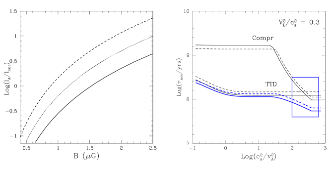
where $\langle\Gamma\rangle$ is the average collisionless TTD damping term given by Eqs.(29), (31) and (33). The value of the cut–off scale is reported in Fig. 5b as a function of the beta of the plasma for physical conditions in the ICM (see caption): we find that if turbulence is energetic enough (actually for the values used in the § 5.3–5.5) compressible modes are dissipated at $\approx$ sub–kpc scales. The cut–off scale slightly increases in the case of small $\beta_{pl}$ as the cascading of magnetosonic modes becomes less efficient (the cascading time–scale goes as $\tau_{kk}\propto\langle V_{\rm ph}\rangle$ and, fixed $c_{s}$, increases for small $\beta_{pl}$). Actually the cascading of compressible motions is likely to reach MHD scales before being dissipated, $l_{cut}\leq l_{A}$ (Fig. 6a), and in this case it is also worth to mention that an Alfvénic turbulence can be activated by the cascading of these compressible motions.

Eq.(41) is appropriate to describe the time evolution of the total spectrum of isotropic turbulent modes. On the other hand, formally in the collisionless regime the ratio between the energy of the fields ($E$ and $B$) and that associated with particles changes with the mode–propagation angle (Figs. 1–2, Appendix B). However the induced anisotropy is within a factor of 2–3 for a stationary $B_{o}$, and it should be efficiently smoothed out by the effect of the bending of the field lines (§ 4.3). Thus we shall adopt isotropy as a viable approximation, and define the energy associated with the magnetic field fluctuations as:

$${\cal W}_{B}(k,t)\sim{1\over{\beta_{pl}}}\langle{{\beta_{pl}|B_{k}|^{2}}\over{16\pi W(k)}}\rangle{\cal W}(k,t)$$ (46)

where for consistency $|B_{k}|^{2}/W$ is taken from Eq.(24) and $\langle\rangle$ indicates the average over the propagation angle of the modes.

The TTD diffusion coefficient in the particle–momentum space is then obtained from Eqs.(40), (43), and (46) in the form :

$$D_{pp}(p,t)={{\pi}\over{8}}\,{{p^{2}}\over{c}}\langle{{\beta_{pl}|B_{k}|^{2}}\over{16\pi W}}\rangle{{1}\over{c_{s}^{2}}}\left({{2I_{o}\langle V_{\rm ph}\rangle}\over{7\rho}}\right)^{{1\over 2}}{k_{cut}(t)}^{{1\over 2}}\int_{0}^{\pi/2}d\theta V_{\rm ph}^{2}{{\sin^{3}(\theta)}\over{|\cos(\theta)|}}{\cal H}\left(1-{{V_{\rm ph}/c}\over{\cos\theta}}\right)\left(1-({{V_{\rm ph}/c}\over{\cos\theta}})^{2}\right)^{2}$$ (47)

Eq.(47) allows a prompt estimate of the acceleration efficiency via TTD resonance, once the injection rate per unit mass of the compressible turbulence ($I_{o}/\rho$) and the injection scale, $k_{o}$ (or $L_{o}$), are fixed :

$${{I_{o}}\over{\rho}}\approx{\cal C}V_{L}^{3}\,k_{o}\left({{V_{L}}\over{\langle V_{\rm ph}\rangle}}\right)$$ (48)

where ${\cal C}\approx 5-6$ is a numerical factor which can be readily obtained by taking $I_{o}/\rho\approx V_{L}^{2}/\tau_{LL}$ and Eq.(44). The resulting systematic acceleration rate, $\tau_{acc}$, is given by :

$$\tau_{acc}=p^{3}\big{\{}{{\partial}\over{\partial p}}\left(p^{2}D_{pp}(p)\right)\big{\}}^{-1}$$ (49)

The systematic acceleration time from TTD resonance does not depend on particle momentum (see also Fig.7) and is reported in Fig.(6b) as a function of $c_{s}^{2}/v_{A}^{2}(=2\beta_{pl})$: for a given temperature (and $\beta_{pl}>1$) the acceleration efficiency scales approximatively with $\sqrt{T}$ and is found to be almost independent from the value of $\beta_{pl}$. The important point here is that the strength of the TTD–acceleration efficiency, powered by compressible turbulence with large–scale rms velocity $V_{L}^{2}/c_{s}^{2}\approx 0.3$, is found to give a systematic acceleration time of the order of $\sim 10^{8}$yrs which is sufficient to accelerate electrons up to energies of several GeV, and this may produce diffuse synchortron radio emission in $\mu$G–magnetized media (§ 6).

5.2 Nonresonant acceleration

5.2.1 Introduction

Resonant TTD acceleration is not the only process by which compressible turbulence may accelerate cosmic rays in the ICM. For instance, fast particles can be accelerated also by large scale compressible motions (e.g., Ptuskin 1988; Chandran 2003; Chandran & Maron 2004; Cho & Lazarian 2006). Compression changes the particle momentum according to :

$${{\partial p}\over{\partial t}}=-{1\over 3}p\,\,\nabla\cdot{\bf V}_{l}$$ (50)

If the medium is neither expanding nor contracting it is $\langle\nabla\cdot{\bf V}_{l}\rangle=0$ and thus particles will not experience regular changes in energy. On the other hand if ${\bf V}_{l}$ is a turbulent field a statistical acceleration effect (analogous to a classical second order Fermi process) may exist. This is essentially because particles would statistically experience more compression than expansion.

5.2.2 Diffusion Coefficient

Limiting to the case $V_{l}^{2}<<c_{s}^{2}$ and provided that the turbulent velocity of the medium has correlation scales much longer than the effective particle mean free path, the diffusion coefficient in the particle momentum space, $D_{pp}$, and the total (turbulent advection and diffusion) spatial diffusion coefficient, $D_{*}$, can be obtained by standard procedure in plasma physics in the quasi–linear approximation. These are (Ptuskin 1988):

$$D_{pp}={2\over 9}p^{2}D\int_{k}{{dyy^{2}{\cal V}(y)}\over{c_{s}^{2}+y^{2}D^{2}}}$$ (51)

and

$$D_{*}=D\left(1+{4\over 3}\int_{k}{{dy{\cal V}(y)}\over{c_{s}^{2}+y^{2}D^{2}}}\right)$$ (52)

where $D$ is the spatial particle–diffusion coefficient (without considering the effects induced by the nonresonant compressible coupling itself, Eq. 51), and ${\cal V}(y)$ is defined as :

$$\int{\cal V}(y)dy=V_{L}^{2}$$ (53)

In this regime slow and fast diffusion limit exist. In the slow limit the rate of particle diffusion out of compressible eddies is slower than the wave period, $\tau_{w}\sim l/c_{s}$, i.e. $\tau_{diff}\sim l^{2}/D>>\tau_{w}$ and $c_{s}^{2}>>k^{2}D^{2}$. Here the process is mainly contributed by the action of the smaller eddies in the spectrum of the modes and it becomes faster as this minimum scale gets smaller (e.g., Cho & Lazarian 2006). From Eq.(51) we find :

$$D_{pp}\sim{1\over 9}p^{2}\left({{V_{L}}\over{c_{s}}}\right)^{2}D\left({1\over{L_{o}l^{2}}}\right)^{2/3}_{l\sim l_{min}}$$ (54)

For small minimum–turbulent scales this process formally becomes extremely efficient, however the minimum scale of the bulk of compressible turbulent eddies in the ICM cannot be very small as these modes are strongly damped (§ 5.1.3, Fig. 5).

In the opposite case, in the fast diffusion limit, particles leave the eddies before they turnover, i.e. $\tau_{diff}<<\tau_{w}$ and $c_{s}^{2}<<k^{2}D^{2}$. Here the process is mainly contributed by the action of the largest eddies which contain the bulk of the turbulent energy, and from Eqs.(51) & (53) we find :

$$D_{pp}\sim{2\over 9}p^{2}{{V_{L}^{2}}\over{D}}$$ (55)

An important point discussed in § 3.2 is that particle–spatial diffusion itself is likely to be affected by the turbulent bending of the magnetic field lines which gets the effective ion mean free path $\sim l_{A}$. Compared to the Coulomb or gyroresonance scattering the diffusion with the characteristic scale $l_{A}$ does not involve any changes of the particle energy via scattering. Therefore the particle may diffuse slowly, but the only change in energy will be due to large scale compressions (cf. Cho & Lazarian 2006). We thus shall adopt a very simplified form of the spatial diffusion coefficient in Eqs.(51–55) :

$$D\sim{c\over 3}\beta\max\Big{\{}l_{cut}\,,\,\min\{l_{A}\,,\,l_{mfp}\}\Big{\}}$$ (56)

The combination between Eqs.(51) and a turbulent–driven spatial diffusion coefficient (e.g., Eq. 56) provides an important refinement of the evaluation of the cosmic–ray acceleration via compressible long wave turbulence, and may have important consequences in the case of the particle acceleration in the ICM (§ 5.3).

Finally, we want to remind that Eq.(51) is obtained by neglecting the effect of possible additional scattering processes due to resonant particle–wave interactions. The presence of instabilities in cosmic rays may create an additional slab-type Alfvénic component that would produce additional gyroresonance acceleration and reduce the effective mean free path (Lazarian & Beresnyak 2006). Conservatively we do not discuss this possibility in the present paper.

Figure 6: Panel a): The ratio $l_{A}/l_{cut}$ is reported as a function of $B$. Calculations are reported for $k_{B}T=$6 keV (dashed lines), 9 keV (dotted lines), and 12 keV (solid lines); $(V_{L}/c_{s})^{2}=0.3$, $n_{th}=10^{-3}$cm^-3, and $L_{o}=$ 300 kpc were assumed in the calculations. Panel b): The acceleration time (Eq. 49) is reported as a function of $c_{s}^{2}/v_{A}^{2}$ in the case of nonresonant compressive acceleration (Eqs. 51) and resonant TTD acceleration (Eq. 47). Calculations are reported for $k_{B}T=$7 keV (dashed lines) and $k_{B}T=$11 keV (solid lines); $(V_{L}/c_{s})^{2}=0.3$, $n_{th}=10^{-3}$cm^-3 , and $L_{o}=$ 300 kpc were assumed in the calculations. The acceleration time from the combined effect of the two mechanisms is also shown (tick lines). The box marks the relevant range of the values of $c_{s}^{2}/v_{A}^{2}(=\beta_{pl}/2)$ in the hot ICM, and the acceleration time necessary to boost relativistic electrons at several GeV (this accounts for both synchrotron and inverse Compton losses with redshift $\sim$0–0.3).

5.2.3 Acceleration efficiency in the ICM

In this Section we calculate the efficiency of the particle acceleration from large–scale nonresonant compression in the ICM.

Taking a Kraichnan scaling for the super–Alfvénic compressible turbulence, ${\cal V}(k)\approx V_{L}^{2}k^{-3/2}/L_{o}^{1/2}$, from Eq.(51) we have :

$$D_{pp}\simeq{2\over 9}D\,p^{2}{{V_{L}^{2}}\over{L_{o}^{1/2}}}\int_{1/L_{o}}^{1/l_{cut}}{{dy\,y^{1/2}}\over{c_{s}^{2}+D^{2}y^{2}}}$$ (57)

where the spatial–diffusion coefficient is given by Eq.(56).

The resulting systematic acceleration time is independent of particle momentum (at least in the ultra–relativistic case, see also Fig. 7) and is reported in Fig. 6b. For a given temperature of the plasma, $T$, in the case of small $\beta_{pl}$ the nonresonant compression is formally very inefficient because for large values of the magnetic field the particle spatial–diffusion coefficient is large (essentially $D\approx 1/3\,\beta\,c\,l_{mfp}$, $l_{mfp}$ from Eq. 1). On the other hand, in the case of large $\beta_{pl}$ the acceleration efficiency increases because turbulence bends the magnetic field lines at scales smaller than $l_{mfp}$ and the effective particle mean free path is $\approx l_{A}$ (which scales as $\beta_{pl}^{-3/2}$); saturation for large $\beta_{pl}$ is reached when $l_{cut}\geq l_{A}$ (Fig. 6).

The reference value of $\beta_{pl}$ in the ICM is in the range $\beta_{pl}\sim 200-1000$ (i.e. $B\sim 0.5-3\mu$G, with $n_{th}\sim 10^{-4}-10^{-3}$cm^-3 and $k_{B}T\sim 7-10$ keV), and formally under these conditions we find that the acceleration efficiency from nonresonant compression driven by relatively energetic turbulence (caption) is similar to that due to the TTD–resonance.

As already pointed out in § 5.2.2, in the derivation of Eq.(51) (or Eq.57) it was assumed that the effective particle mean free path is much smaller than the scale of the turbulent eddies. This condition is formally violated in the case of small $\beta_{pl}$ in Fig. 6b where the smaller turbulent eddies are $<l_{mfp}$ (mean free path $l_{mfp}\approx 10-50$ kpc). On the other hand, this does not happen for larger $\beta_{pl}$, since in this case the particle effective mean free path, $\approx l_{A}\approx l_{cut}$, is actually comparable to (or smaller than) the smallest turbulent eddies.

5.3 Overall effect of compressible turbulence

As discussed in § 5.1.1 the TTD resonance is expected to be an efficient mechanism in the ICM, provided that particle isotropy is preserved. Yet the TTD alone might not be efficient enough in maintaining such isotropy because both $D_{pp}(\mu,p)$ and $D_{\mu\mu}(\mu,p)$ are strongly maximized for particles moving at small angles with the direction of the seed magnetic field. However additional resonant processes acting on small scales might easily maintain particle isotropy. If these mechanisms are really at work in the ICM they should also affect the spatial diffusion, $D$, of the particles and thus the efficiency of the nonresonant compression mechanism. Formally with decreasing $D$ the nonresonant coupling with eddies in the fast diffusion limit becomes more efficient, and, at the same time, a larger range of scales of the eddies couples with particles in the slow diffusion regime which is very efficient; actually this is what happens with increasing the beta of the plasma in Fig. 6b. However, if the spatial diffusion is strongly suppressed, namely when $D<c_{s}l_{cut}$ in Eqs.(51) and (57), one gets into the slow diffusion limit at any turbulent scale, and a decrease of $D$ yields a corresponding decrease in the efficiency of the nonresonant compression (Eq. 54). Thus future studies using self–consistent spatial diffusion coefficients will be of great importance.

The turbulent bending of the field lines which happens in the super–Alfvénic case cannot change the pitch angle of particles which would preserve the adiabatic invariant, however in the high beta ICM turbulent bending is associated with turbulent compressions which indeed power the nonresonant acceleration mechanism and might provide a source of particle–pitch angle isotropization. The spatial diffusion coefficient is related to that in the pitch angle as (order of magnitude) $D\approx c^{2}/D_{\mu\mu}$, and the resulting time–scale of the pitch angle scattering, $\approx D_{\mu\mu}^{-1}$, is indeed much shorter than the acceleration time of fast particles (which is $\approx 10^{7}-10^{8}$yrs).

This is important since it implies that the action of large scale compressible turbulence in the ICM is twofold. On one hand particles diffusing through the compressible turbulent eddies experience substantial nonresonant stochastic acceleration. On the other hand, even without requiring additional processes at small scales, this might contribute to help in maintaining particle–momentum isotropization, so that the compressive component of the turbulent magnetic field (that along ${\bf B}_{o}$) may also couple efficiently with particles via TTD resonance without greatly change the particle spatial diffusion.

These two mechanisms, TTD resonance and nonresonant compression, are driven by the same turbulent modes and involve independent particle–mode couplings and thus, as a first approximation, the acceleration process may be thought as the combination of the two effects; the deriving particle acceleration time is also reported in Fig.(6b).

6 Compressive turbulence and particle re–acceleration model in galaxy clusters

As already anticipated in the Introduction direct evidence for relativistic electrons diffused on Mpc scales in the ICM comes from radio halos and relics (e.g., Feretti 2005), while the hard X–ray tails detected in a few clusters may result from inverse Compton scattering of the Cosmic Microwave Background photons by the same electrons (e.g., Fusco–Femiano et al. 2004; Rephaeli, Gruber & Arieli 2006).

The particle re–acceleration model is a promising possibility to explain the properties of the giant radio halos and possibly also the strength of the hard X–ray tails. This scenario assumes that turbulence is injected in a substantial fraction, Mpc³, of the cluster volume during cluster–cluster mergers, and that relativistic electrons already present in the ICM and accumulated at $\gamma\approx 100$ are re–accelerated for a typical time–scale of $\leq$Gyr (e.g., Brunetti et al. 2001,04; Petrosian 2001; Fujita et al. 2003). Alternatively these seeds electrons to be re–accelerated could be secondary products of hadronic interactions (Brunetti & Blasi 2005).

In this Section, after a brief review of the injection processes of cosmic rays in galaxy clusters and of the most relevant channels of energy losses (§ 6.1), we provide calculations in the context of the particle re–acceleration model which include the effect of TTD–resonance and nonresonant acceleration due to compressible turbulent modes injected at large scales.

6.1 Cosmic Ray injection in the ICM

There is a general consensus on the fact that several mechanisms of injection of cosmic rays may be at work in the ICM, and that once injected the bulk of these cosmic rays does not escape the cluster (e.g., Berezinsky, Blasi & Ptuskin 1997; Ensslin et al. 1998; Voelk & Atoyan 1999).

Collisionless shocks are generally recognized as efficient particle accelerators through the so-called diffusive shock acceleration (DSA) process (Drury, 1983; Blandford & Eichler 1987). This mechanism has been invoked several times as an efficient acceleration process in clusters of galaxies (Takizawa & Naito 2000; Blasi 2001; Miniati et al. 2001; Fujita & Sarazin 2001; Ryu et al. 2003). Present simulations confirm the analytical claim that shocks with Mach number larger than 2–3 are rare (Gabici & Blasi 2003), and claim that the energy content in the form of cosmic rays in massive clusters may be of the order of a few percent of the thermal energy (Pfrommer et al. 2006; Jubelgas et al. 2006). The bulk of the energy of these cosmic rays is injected in the cluster outskirts by shocks with a Mach number of the order of $\sim 3$, the real efficiency of these shocks is however uncertain and it is generally computed in the test particle limit and according to the so-called thermal leakage model (e.g., Kang & Jones, 1995).

A contribution to the injection of cosmic rays in clusters of galaxies may come from Active Galactic Nuclei which indeed might fill the ICM with relativistic particles and magnetic fields, extracted from the accretion power of their central black hole (Ensslin et al., 1997). Similarly to Active Galactic Nuclei, powerful Galactic Winds may also inject relativistic particles and magnetic fields in the ICM (Völk & Atoyan 1999). Although the present day level of starburst activity is low, it is expected that these winds were more powerful during starburst activity in early galaxies, as also suggested by the iron abundances in galaxy clusters (Völk et al. 1996).

6.2 Energy Losses

6.2.1 Electrons and Positrons

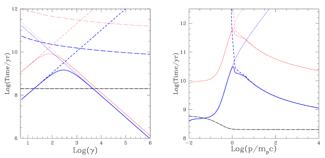
In the conditions typical of the ICM, ultra-relativistic electrons rapidly cool down through inverse Compton and synchrotron emission, and accumulate at Lorentz factors $\gamma\sim 100-500$ where they may survive for a few billion years before cooling further down in energy through Coulomb scattering and eventually thermalize. Energy losses and relevant time–scales of relativistic electrons in the ICM are discussed in several papers (e.g., Sarazin 1999; Petrosian 2001; Brunetti et al. 2004; Pfrommer & Ensslin 2004). In Fig. 7a we report the particle life–time as a function of the Lorentz factor: the life–time has a peak at $\gamma\approx 10^{2}-10^{3}$ where the cooling of electrons is slower and where particles may accumulate providing a seed populations to be re–accelerated in the context of the re–acceleration model. More specifically, Fig. 7a is obtained for typical physical conditions in cluster cores and in the cluster outskirts: in the external regions of clusters electrons survive since Coulomb losses are less severe and in principle these particles can be accumulated for cosmological time–scales at energies $\gamma\sim 100-1000$. On the other hand, in cluster cores the higher thermal density limits the maximum life–time of electrons at less than 1 Gyr.

6.2.2 Protons

Once injected the relativistic cosmic–ray protons do not suffer catastrophic radiative–energy losses. The only relevant channel of energy losses for these particles in the ICM is given by hadronic collisions which however get a typical particle life–time which is larger than a Hubble time for $\sim$ GeV particles. This, together with the long time necessary to the bulk of these cosmic rays to diffuse out of clusters, makes clusters themselves reservoir in which cosmic ray protons are confined and may accumulate over cosmological epochs (e.g., Völk et al. 1996; Berezinsky, Blasi & Ptuskin 1997).

On the other hand, mildly and sub- relativistic protons may be significantly affected by Coulomb energy losses, which in turn change the particle spectrum with respect to the injection spectrum. The rate of Coulomb losses is (e.g., Schlickeiser 2002) :

$${{dp}\over{dt}}_{i}(\beta_{p})\approx-{{6}\over{\sqrt{\pi}}}\times 10^{-29}n_{th}\left[\int_{0}^{\beta_{p}/\beta_{e}}dy\exp\{-y^{2}\}-{{\beta_{p}}\over{\beta_{e}}}\left(1+{{m_{e}}\over{m_{p}}}\right)\exp\big{\{}-({{\beta_{p}}\over{\beta_{e}}})^{2}\big{\}}\right]$$ (58)

where $\beta_{p}$ and $\beta_{e}\sim 0.18(T/10^{8}K)^{1/2}$ are the velocity in units of the light speed of thermal electrons in the ICM and of the cosmic ray protons, respectively.

As in the case of leptons, the details of the mechanisms of energy losses of cosmic ray hadrons in the ICM can be found in several papers (e.g., Blasi & Colafrancesco 1999; Pfrommer & Ensslin 2004; Brunetti & Blasi 2005). In Fig. 7b we report the particle life–time as a function of the particle momentum. Fig. 7b is obtained for typical physical conditions in cluster cores and in the cluster outskirts: it is clear that even in the cluster cores where losses are much severe, the bulk of relativistic protons has a life–time of the order of an Hubble time. Only protons with kinetic energy larger than about 200 GeV and smaller than about 30 MeV in the cluster cores have life–times smaller than a couple of Gyrs, while just out of the core regions the life–time of these particles grows (time $\propto n_{th}^{-1}$) and all these particles are expected to survive for cosmological time–scales.

Figure 7: Left panel: The life–time of relativistic electrons in the ICM at $z=0.2$ as a function of the Lorentz factor. Thick (blue) lines are for cluster cores and thin (red) lines are for cluster periphery. We report the total life–time (solid lines) and the life–times due to single processes: Coulomb losses (dashed lines), synchrotron and IC losses (dotted lines), and bremsstrahlung losses (long dashed lines). Right panel: The life–time of cosmic–ray protons in the ICM at $z=0.2$ as a function of the particle momentum. Thick (blue) lines are for cluster cores and thin (red) lines are for cluster periphery. We report the total life–time (solid lines) and the life–times due to single processes: Coulomb losses (dotted lines) and pp–collisions (dashed lines). In both panels calculations in the cores (thick–blue) are obtained for $B=3\mu$G and $n_{th}=2\times 10^{-3}$cm^-3, and in the periphery (thin–red) for $B=0.5\mu$G and $n_{th}=10^{-4}$cm^-3. For comparison, the dash–dotted lines in both panels give the acceleration time–scale which is used in Fig.8; note that the increase of this time–scale in the case of sub–relativistic protons is due to the decrease of the efficiency of the non–resonant compression at sub–relativistic energies.

Figure 8: Left Panel: Time–evolution of the spectrum of relativistic electrons as a function of the Lorentz factor. Right Panel: Time–evolution of the spectrum of cosmic ray protons as a function of the particle momentum. In both panels calculations are reported for: $t=0$, $4\times 10^{15}$, $8\times 10^{15}$, $10^{16}$, $1.2\times 10^{16}$sec from the start of the re–acceleration phase. Calculations are performed assuming $(V_{L}/c_{s})^{2}=0.18$, $L_{o}=300$ kpc, $n_{th}=10^{-3}$, $k_{B}T$=9 keV, $B=1\mu$G, and redshift z=0.1 (for IC losses).

6.3 Numerical Calculations

In this Section we calculate the time–evolution of the spectrum of the relativistic particles stochastically re–accelerated by turbulent modes in the ICM.

6.3.1 Formalism

As discussed in § 5 we shall assume isotropy of the particle momenta and of the modes, and in this case the time evolution of the spectrum of the turbulent modes and of the particles can be formally derived by a set of coupled kinetic equations. The time evolution of the spectrum of the leptonic component is given by :

$${{\partial N_{\pm}(p,t)}\over{\partial t}}={{\partial}\over{\partial p}}\left[N_{\pm}(p,t)\left({{dp}\over{dt}}_{\rm rad}+{{dp}\over{dt}}_{\rm i}-{2\over{p}}\big{\{}D^{r}_{\rm pp}+D^{c}_{\rm pp}\big{\}}\right)\right]+{{\partial}\over{\partial p}}\left[\big{\{}D^{r}_{\rm pp}+D^{c}_{\rm pp}\big{\}}{{\partial N_{\pm}(p,t)}\over{\partial p}}\right]+Q_{e^{\pm}}(N_{p}(p,t);p,t)\,,$$ (59)

where $N_{-}$ and $N_{+}$ stands for electrons and positrons ($N=4\pi p^{2}f$, $f$ is used in § 4), respectively, and where the terms $dp/dt_{rad}$ and $dp/dt_{i}$ account for radiative (synchrotron and IC) and Coulomb losses, while $D^{r}_{pp}$ and $D^{c}_{pp}$ are the resonant (TTD, Eq.47) and the non–resonant (from turbulent–compression, Eq. 57) particle momentum–diffusion coefficients. In Eq. 59 we also formally include an injection term, $Q_{e^{\pm}}(N_{p}(p,t);p,t)$, which depends on the spectrum of cosmic ray protons, and is necessary in the case that the re–accelerated electrons and positrons are injected by hadronic collisions in the ICM (see Brunetti & Blasi 2005).

The time evolution of the spectrum of cosmic ray protons is given by :

$${{\partial N_{p}(p,t)}\over{\partial t}}={{\partial}\over{\partial p}}\left[N_{p}(p,t)\left({{dp}\over{dt}}_{\rm i}-{2\over{p}}\big{\{}D^{r}_{\rm pp}+D^{c}_{\rm pp}\big{\}}\right)\right]+{{\partial}\over{\partial p}}\left[\big{\{}D^{r}_{\rm pp}+D^{c}_{\rm pp}\big{\}}{{\partial N_{p}(p,t)}\over{\partial p}}\right],$$ (60)

where the term $dp/dt_{i}$ accounts for Coulomb losses (Eq. 58), while the particle depletion due to proton–proton collisions can be neglected. Because the population of cosmic ray protons in the ICM essentially comes from the accumulation of these particles during cosmological time–scales, we do not consider the source term in Eq.(60) which would account for the contribution from freshly injected protons.

The evolution of the spectrum of the compressible turbulent modes is given by Eq.(41) described in § 5.1.3, where all the dampings are formally derived in combination with Eqs.(59–60). The effect of the non–resonant damping on the spectrum of the modes can be neglected since turbulent–compression acts efficiently only on relativistic particles in the ICM (§ 5.2), and this gets a net damping rate which is much smaller than that via TTD–resonance with the thermal ICM.

6.3.2 Assumptions

In this paper we adopt the particle re–acceleration model assuming that a seed population of relativistic electrons and protons in the ICM is re–accelerated by turbulence injected at large scales during a merger event. For simplicity we do not study the more complex issue of the re–acceleration of secondary electrons and positrons injected by proton collisions in the ICM (Brunetti & Blasi 2005).

The new of this paper is that compressible turbulence is used as the driving of particle re–acceleration, and accordingly the detailed diffusion coefficients obtained in § 5 and the scenario and properties of turbulence discussed in § 3-4 are used in the calculations. For seek of clarity the main assumptions and physical parameters used in the calculations are listed below :

• i) We consider physical parameters appropriate for massive galaxy clusters: $T\approx 10^{8}$K, $n_{th}\approx 10^{-3}$cm^-3, $B\approx 0.5-3\,\mu$G.

• ii) Turbulence is assumed to be sub–sonic, with $V_{L}^{2}<<c_{s}^{2}$, and injected at large scales $L_{0}\approx 300-500$ kpc for a typical cluster–cluster crossing time.

• iii) The initial spectrum of electrons, $N_{e}(p,t=0)$, is derived by assuming that electrons are injected in the ICM in a single event and then evolve passively for $\approx 1-3$ Gyr before being re–accelerated (see Brunetti et al. 2004).

• iv) The initial spectrum of protons, $N_{p}(p,t=0)$, is derived by assuming that protons are continuously injected in the ICM for a long period, $\approx 3-5$ Gyr, with a constant injection spectral rate $Q\propto p^{-2.2}$ before being re–accelerated (see Brunetti et al. 2004).

• v) Damping terms from relativistic species in Eq.(41) are neglected in the calculations as they become important only if the relativistic component gets a relevant fraction of the thermal energy of the ICM (§ 4.3).

• vi) The damping term due to thermal particles is taken stationary because, under the assumption (ii), the thermal properties of the ICM are not significantly modified with time.

Under conditions ii), v) and vi) the spectrum of the modes is also stationary and this is given by Eq.(43).

6.3.3 Main Results

Once large scale turbulence is injected in the ICM, magnetosonic modes take a relatively long time to cascade at collisionless scales :

$$\tau_{kk}({\rm Gyr})\approx 0.6\left({{L_{o}}\over{300\,{\rm kpc}}}\right)\left({{V_{L}}\over{10^{3}{\rm km/s}}}\right)^{-1}\left({{M_{s}}\over{0.5}}\right)^{-1}$$ (61)

In the re–acceleration scenario this is an unavoidable temporal gap, of a fraction of a Gyr, between the injection of the first turbulent eddies and the beginning of the particle re–acceleration process. When turbulence reaches collisionless scales the acceleration process starts and particles take a time, of the order of the re–acceleration time, to be significantly boosted in energy. A relevant example of the time evolution of the electron and proton spectrum during the re–acceleration period is reported in Fig. 8 assuming $V_{L}^{2}\sim 0.18\,c_{s}^{2}$ (see caption): the seed electrons initially accumulated at $\gamma\sim 10^{2}-10^{3}$ are efficiently re–accelerated up to $\gamma\approx 10^{4}-10^{5}$.

Radio (and hard X–rays) observations can be well explained in terms of a high energy tail of emitting relativistic electrons at energies of several GeV (e.g. Schlickeiser et al. 1987; Brunetti et al. 2001; Petrosian 2001). We calculate the evolution of the re–accelerated particles under the conditions given in § 6.3.2 and find that, quite independently from the initial electron and proton spectrum, an appreciable high energy tail of relativistic electrons at these energies is produced approximatively for $(V_{L}/c_{s})^{2}\geq 0.15(1+z/0.1)^{2}$. In this case compressible turbulence injected at large scales in galaxy clusters may actually trigger efficient particle re–acceleration, and potentially explain the diffuse Mpc radio sources observed in massive galaxy clusters and the hard X–rays in excess to the thermal X–ray emission.

A spectral break, at $\approx$GHz frequencies, is observed in the synchrotron spectrum of a few radio halos and this is interpreted in favour of the re–acceleration scenario (e.g., Brunetti 2004; Feretti 2005). Under the conditions i) in Sect. 6.3.2, such a break requires the presence of a corresponding break in the spectrum of the emitting electrons at energies $\approx$5–10 GeV, and we find that this is reproduced by our re–acceleration model in the case of moderate turbulence, typically $(V_{L}/c_{s})^{2}\sim 0.15-0.25$, while in the case of more energetic turbulence electrons can be re–accelerated at larger energies and the corresponding synchrotron break is shifted at several GHz.

Also protons are efficiently re–accelerated. Relativistic protons are not subject to radiative losses and since the re–acceleration efficiency scales with the energy of the particles (§ 5.1–5.2) the spectrum is simply shifted at higher energies and the slope of the injection spectrum is essentially preserved during the re–acceleration (Fig. 8).

Under our assumptions (v), § 6.3.2), it is $\Gamma_{th}>>\Gamma_{rel}$ and the spectrum of the turbulent fluctuations in terms of magnetic field, ${\cal W}_{B}$, does not depend on the presence of cosmic rays, thus protons cannot significantly affect the acceleration process of relativistic electrons. This marks an important difference with Alfvénic re–acceleration, in which case the dominant damping of the modes comes from the resonance with relativistic protons and thus these protons affect the electron acceleration (Wave–proton Boiler, Brunetti et al. 2004).

An additional point to stress here is that, because $\Gamma_{th}>>\Gamma_{rel}$, the fraction of the turbulent energy which goes into the cosmic rays via TTD–resonance is simply $\approx\Gamma_{rel}/\Gamma_{th}$ and is fixed by the fraction of the energy in the ICM which is in the form of cosmic rays. An additional contribution to the energy of the re–accelerated particles comes from the non–resonant compression. In our calculations (assuming that cosmic rays store a few percent of the thermal energy in the ICM) the total fraction of the turbulent energy which goes into non–thermal particles is of the order of $\approx 2-5\%$.

In case of long re–acceleration periods, actually $\geq 3-4$ times the re–acceleration time (Eq. 49), a non negligible fraction of the electron number is boosted toward the maximum energy. Here an equilibrium between acceleration and losses is reached and most of the energy flux from the damping of the turbulence with these particles is radiated away via synchrotron and IC by the same re–accelerated particles. Thus in principle for very long re–acceleration periods the total energy of the electron population should saturate and the spectrum is expected to slowly approach stationary conditions. On the other hand since cosmic ray protons are free from energy losses, the energy flux from the damping of the turbulence is totally stored in the form of particle energy and this gives an unbalance between electron and proton acceleration. In the re–acceleration scenario this unbalance is not expected to be large, indeed turbulence is injected during cluster mergers and the duration of a re–acceleration period is constrained by the cluster–cluster crossing time and by the turbulence cascading time, and these cannot significantly exceed about 1 Gyr (see Eq. 61). In addition, present studies of the number counts of giant radio halos in galaxy clusters limit the life–time of these sources at about $\approx 1$ Gyr (e.g., Hwang 2004) and this additionally constraints the duration of stochastic particle re–acceleration periods in galaxy clusters. Actually, given these limits, we find that assuming $(V_{L}/c_{s})^{2}\sim$ 0.15–0.25 (which is required to provide the necessary electron re–acceleration up to $\approx 5-10$ GeV) and a duration of the re–acceleration phase in the range 0.4–1 Gyr, the total energy of the cosmic ray protons and that of the relativistic electrons are both boosted by a factor 1.5–4, and the unbalance is not substantial.

7 Discussion

7.1 Major Results

The problem of proton and electron stochastic re–acceleration by compressible motions is a complex one. The efficiency of acceleration depends on the spectrum of compressible turbulent motions. The extend and the shape of this spectrum, in its turn depends on the processes of plasma damping. In the case of the hot ICM the corresponding issues have not yet been clarified sufficiently in the literature.

As a result, we had to address those issues one by one. Namely, we started with the problem of describing turbulence in ICM in § 3. First of all, we provided arguments suggesting that turbulence is expected to be present in the medium in hot (and massive) galaxy clusters. This is also because the ICM is magnetized and this implies a partial suppression of the plasma viscosity. The suppression of the viscosity in a magnetized medium is a well known effect and has been addressed at least for laminar flows (e.g., Simon 1955). In the case of the strongly super–Alfvénic turbulence in the ICM an additional effect comes due to the bending of the field lines. Field lines are bended on scales $<l_{mfp}$ and this affects the ion diffusion process and thus viscosity. An additional suppression of the viscosity might come from the effect of plasma instabilities which affect the ion–ion mean free path, but that are not considered in this paper. Then, as we are interested in the compressible motions we discussed their generation in super–Alfvénic and MHD turbulence along with providing the estimates for collisional and collisionless damping of such motions. The outcome of § 3 is a validation of a basic features of scenario according to which the energy can be injected due to cluster mergers on large scales and energize the particles in the ICM.

The quantitative treatment of the particle re–acceleration requires a much more rigorous treatment of mode spectrum and damping which was non trivial. In § 4 we make use of collisionless physics and quasi–linear theory and derive general formulae for the spectrum of the compressible modes, basically the ratio between the energy in magnetic fluctuations and the total energy in the mode, and for the damping rate in magnetized plasma, and re–obtained expressions known in the literature, as a particular cases of our approach. The importance of the derived formulae goes beyond our particular case of study, as a rigorous description of damping is important for many other astrophysical important situations, e.g. in galactic environments (see Yan & Lazarian 2004).

Having at hand a description of compressible super–Alfvénic and MHD turbulence with specified injection and damping scales we studied in § 5 proton and electron stochastic re–acceleration by compressible modes. We focus on particle acceleration from magnetosonic modes and neglect the contribution from slow modes and Alfvén modes. Slow modes are sub–dominant for particle re–acceleration as they have a phase velocity $<<$ than that of fast modes and sound waves, in addition both slow modes and Alfvén modes get anisotropic at small scales (if injected at large scales) and this reduces the efficiency of gyro–resonance acceleration. We showed that because of efficient damping of fast modes at small scales the acceleration by gyroresonance is suppressed, i.e. only extremely high energy protons with large gyroradius can find magnetic perturbations to resonate with. Thus we study stochastic re–acceleration by both non–resonant large scale compressions and resonant TTD, and clarified the regimes when the non–resonant large scale compressions is important. The acceleration picture that is drawn from this paper is complex. In the case of super–Alfvénic turbulence in the ICM the turbulent bending of magnetic field lines limits particle spatial diffusion. Because line bending is associated with turbulent compression fast particles diffusing through the compressible turbulent eddies may experience efficient stochastic acceleration via Fermi II nonresonant–turbulent compression. The same particles can also experience coupling with these compressible eddies via TTD resonance which is found to be efficient in the ICM provided that particle pitch–angle isotropization is maintained.

Finally, in § 7, we apply our results to the case of the particle re–acceleration scenario which is proposed to explain radio halos (and hard X–ray tails) in galaxy clusters. Our calculations showed that the acceleration of energetic particles in galaxy clusters may be efficient. Relativistic electrons in the ICM can be re–accelerated against radiative and Coulomb losses up to energies of several GeV (or more) assuming that compressible turbulence at large scales stores a non–negligible fraction of the thermal energy, namely $(V_{L}/c_{s})^{2}\geq 0.15$. These electrons would emit Mpc–scale synchrotron radiation up to GHz frequencies (or more) provided that the magnetic field in the ICM is at $\approx\mu$G level on these scales. In addition it also comes out that the re–acceleration of these electrons happens without transferring too much energy to protons, which might alleviate possible problems of earlier re–acceleration models that appealed to Alfvén modes.

7.2 Simplifying assumptions

In other words, the proposed re–acceleration scenario, which makes use of compressible modes, is a plausible one and deserves further studies. At the moment it includes several simplifications. In particular, plasma instabilities can decrease further mean free path of protons, which would decrease damping of turbulence. As a result, compressible modes could cascade to smaller scales, making, for instance, gyroresonance acceleration by fast modes more efficient. An effect related to the gyrokinetic instability in accelerated particles (Lazarian & Beresnyak 2006) may act in a different direction suppressing compressible motions at small scales, however on the other hand the Alfvénic component generated by this instability may also accelerate particles. Plasma instabilities might also affect the diffusion of fast particles and this might be important in the calculation of the efficiency of the acceleration from nonresonant compression.

In addition, reconnection processes taking place in the magnetized plasma should be able to accelerate particles on their own. Within small volume current sheets, the percentage of accelerated particles is small. However, stochastic reconnection model in Lazarian & Vishniac (1999) allows acceleration of a substantial part of particles at the expense of the magnetic energy in the turbulent plasmas (Gouveia Dal Pino & Lazarian 2005). Therefore we believe that our treatment would underestimate the actual acceleration; further research should clarify the actual picture.

Our derivations of the damping rates are valid when the ratio of the imaginary to the real part of the mode–frequency is much less than unity. This is generally true in the ICM and is a natural assumption for dealing with turbulence cascade, as in the opposite regime, no cascading is possible and the energy dissipates at the injection scale.

7.3 Relation to Earlier Works

Stochastic particle acceleration in galaxy clusters has been addressed by several papers (e.g., Schlickeiser et al. 1987; Brunetti et al. 2001; Petrosian 2001; Fujita et al. 2003). This work appeals to compressible motions to re–accelerate particles in the ICM. Earlier detailed time–dependent calculations of the problem of re–acceleration was addressed in Brunetti et al. (2004) and Brunetti & Blasi (2005), where Alfvén modes were used for the purpose. Such an approach is adequate if, for instance, Alfvén modes are injected by some mechanism at small scales. One possibility is that this might happen in the gyrokinetic instability scenario (Lazarian & Beresnyak 2006), and this provides an interesting possibility that we consider elsewhere. If, however, Alfvén modes are injected at large scales the Alfvénic component at the scale of energetic particle gyroradius gets very anisotropic and interacts very inefficiently with the particles (Chandran 2000; Yan & Lazarian 2002). Thus fast compressible modes should be considered. These modes are isotropic and may scatter particles efficiently as we have demonstrated above.

In some aspects the scenario suggested in the present paper for the ICM is similar to that adopted to calculate the scattering of galactic cosmic rays in Yan & Lazarian (2004), and to that adopted in the ICM by Cassano & Brunetti (2005).

The present paper is a theoretical extension of the work of Cassano & Brunetti (2005) where a more simplified treatment of the resonant TTD re–acceleration of electrons by fast modes was used to derive the statistical properties of non–thermal emission in galaxy clusters.

Yan & Lazarian (2004) discuss cosmic rays propagation in Milky Way thus focusing on MHD turbulence at scales $l<l_{A}$ and mostly low beta plasma. On the other hand, here we concentrated on the acceleration by motions at scales larger than $l_{A}$ and high beta plasma, the conditions which are relevant to the clusters of galaxies. This made our calculations of the particle–mode damping rates and of the particle–diffusion coefficients different from those in Yan & Lazarian (2004). In particular, we had to re–adopt many of the plasma results for high beta plasma and to treat differently magnetic field wandering.

Finally, an additional new of this paper is that we not only considered acceleration of electrons by the TTD resonance, but acceleration of fast protons and electrons subjected to both the TTD resonance and the large scale compressions.

8 Short Summary

The paper above explains the non-thermal emission observed in galaxy clusters as a consequence of electron re–acceleration by compressible turbulence. In this scenario turbulence is injected at the scale of galaxy mergers and cascades to small scales where the bulk of energetic particle acceleration happens. The turbulence is described by using the recent advances in understanding of MHD turbulence. The paper incorporates:
I. A model of compressible turbulence in galaxy clusters. In this model the energy is injected at the scale of galaxy mergers and cascades to small scales where the bulk of energetic particle acceleration happens.
II. Calculations of the plasma damping and energy of the mode for an arbitrary angle of wave propagation to magnetic field and a rather general model of plasma.
III. Calculations of acceleration of protons and electrons by compressible motions in ICM plasma and a detailed application to the particle re–acceleration scenario to explain radio halos and possibly hard X–ray tails.

Our results show that electrons obtain a substantial part of the energy transfered to the energetic particles, which fits well to the existing observational constraints.

9 Acknowledgments

We thank the referee V. Petrosian for very useful comments and discussions, and R. Cassano and V. Dogiel for comments on the manuscript. We acknowledge partial support from MIUR through grant Cofin2004. GB thanks partial support from MIUR through grant PRIN2005. AL acknowledges NASA NNG05GGF57G and the NSF Center for Magnetic Self–Organization in Laboratory and Astrophysical Plasmas.

Appendix A Dielectric Tensor in the long wavelength limit

A relevant case for many astrophysical situations is that of long–wavelength modes for which it is $|z_{\alpha}|\sim kp/m_{\alpha}\Omega_{o}^{\alpha}<<1$. This is also the case of the turbulent modes in the ICM of interest in the present paper. The dielectric tensor (Eq.16) is in the form :

$$K_{ij}=\delta_{ij}-\omega^{-2}\sum_{\alpha}R^{\alpha}_{ij}$$ (62)

Barnes & Scargle (1973) calculated the tensor $R_{ij}$ from Eqs.16–17 and under the conditions $z_{\alpha}=k_{\perp}p_{\perp}/m_{\alpha}\Omega^{\alpha}_{o}<<1$ and $X^{\alpha}_{1}\equiv(k_{\|}p_{\|}/m_{\alpha}-\omega\gamma)/\Omega^{\alpha}_{o}<<1$. In this case, by taking into account that $J_{n}(z_{\alpha})=(z_{\alpha}/2)^{n}\sum_{m}(-z_{\alpha}^{2}/4)^{m}/m!\Gamma(n+m+1)$, one finds (BS73) :

$$R_{ij}\simeq-2\pi\sum_{\alpha}\omega_{p,\alpha}^{2}\int_{o}^{\infty}dp_{\perp}\int_{-\infty}^{\infty}dp_{\|}\Big{\{}p_{\perp}^{2}\Lambda^{\alpha}_{ij}\Big{[}(\omega-k_{\|}v_{\|})\cdot{{\partial\hat{f}_{\alpha}(p)}\over{\partial p_{\perp}}}+k_{\|}v_{\perp}{{\partial\hat{f}_{\alpha}(p)}\over{\partial p_{\|}}}\Big{]}+m_{\alpha}p_{\|}\Big{(}v_{\perp}{{\partial\hat{f}_{\alpha}(p)}\over{\partial p_{\|}}}-v_{\|}{{\partial\hat{f}_{\alpha}(p)}\over{\partial p_{\perp}}}\Big{)}\delta_{i3}\delta_{j3}\Big{\}}$$ (63)

where

$$\Lambda^{\alpha}_{ij}={1\over{2\Omega_{o}^{\alpha}}}\pmatrix{X_{1}^{\alpha}&-{\it i}&-\Big{(}{{p_{\|}}\over{p_{\perp}}}\Big{)}z_{\alpha}\cr{\it i}&X_{1}^{\alpha}-{{z_{\alpha}^{2}}\over{2X_{1}^{\alpha}}}&-{\it i}\Big{(}{{p_{\|}}\over{p_{\perp}}}\Big{)}{{z_{\alpha}}\over{X_{1}^{\alpha}}}\cr-\Big{(}{{p_{\|}}\over{p_{\perp}}}\Big{)}z_{\alpha}&{\it i}\Big{(}{{p_{\|}}\over{p_{\perp}}}\Big{)}{{z_{\alpha}}\over{X^{\alpha}_{1}}}&{{z_{\alpha}^{2}-2}\over{X_{1}^{\alpha}}}\Big{(}{{p_{\|}}\over{p_{\perp}}}\Big{)}^{2}\cr}+{\cal O}(z_{\alpha}^{2})$$ (64)

and where the term ${\cal O}(z_{\alpha}^{2})$ comes from the contribution from the $n\geq 2$ resonances in Eq.(16).

In an isotropic plasma, Eqs.(63–64) can be further simplified by introducing the total energy of species $\alpha$ :

$${\cal E}_{\alpha}=2\pi N_{\alpha}\int\int dp_{\perp}p_{\perp}dp_{\|}\hat{f}_{\alpha}(p)m_{\alpha}c^{2}\gamma\,,$$ (65)

and the pressure of species $\alpha$ :

$${P}_{\alpha}={P}_{\perp}^{\alpha}=\pi N_{\alpha}\int\int dp_{\perp}p_{\perp}dp_{\|}\hat{f}_{\alpha}(p)p_{\perp}v_{\perp}={P}_{\|}^{\alpha}=2\pi N_{\alpha}\int\int dp_{\perp}p_{\perp}dp_{\|}\hat{f}_{\alpha}(p)p_{\|}v_{\|}\,.$$ (66)

which is $P_{\alpha}=N_{\alpha}k_{B}T$ for a Maxwellian distribution of $\alpha$ particles.

By integrating Eqs. 63–64, introducing Eqs.(65–66), and requiring no net charge in the plasma (i.e., $\sum_{\alpha}N_{\alpha}e_{\alpha}=0$), the components of the tensor are given by :

$$R_{11}=-{{4\pi k_{\|}^{2}c^{2}}\over{B_{o}^{2}}}\left({{\omega}\over{k_{\|}c}}\right)^{2}\sum_{\alpha}\left({\cal E}_{\alpha}+{P}_{\alpha}\right)$$ (67)

$$R_{12}=R_{21}=0$$ (68)

$$R_{13}=R_{31}=0$$ (69)

$$R_{22}=R_{11}+{{8\pi k_{\perp}^{2}c^{2}}\over{B_{o}^{2}}}\sum_{\alpha}{P}_{\alpha}-\sum_{\alpha}{{\pi k_{\perp}^{2}N_{\alpha}}\over{B_{o}^{2}}}\langle p_{\perp}v_{\perp}^{3}\rangle_{\alpha}-{{2\pi^{2}k_{\|}k_{\perp}^{2}c^{2}}\over{B_{o}^{2}}}\sum_{\alpha}N_{\alpha}\int\int p_{\perp}dp_{\perp}dp_{\|}{{p_{\perp}^{2}v_{\perp}^{2}}\over{\omega-k_{\|}v_{\|}}}{{\partial\hat{f}_{\alpha}(p)}\over{\partial p_{\|}}}$$ (70)

$$R_{23}=-R_{32}=-{{4\pi^{2}{\it i}k_{\perp}c}\over{B_{o}}}\sum_{\alpha}N_{\alpha}e_{\alpha}\omega\int\int p_{\perp}dp_{\perp}dp_{\|}{{p_{\perp}v_{\perp}}\over{\omega-k_{\|}v_{\|}}}{{\partial\hat{f}_{\alpha}(p)}\over{\partial p_{\|}}}$$ (71)

$$R_{33}=-{{8\pi^{2}\omega^{2}}\over{k_{\|}}}\sum_{\alpha}N_{\alpha}e_{\alpha}^{2}\int\int p_{\perp}dp_{\perp}dp_{\|}{{1}\over{\omega-k_{\|}v_{\|}}}{{\partial\hat{f}_{\alpha}(p)}\over{\partial p_{\|}}}$$ (72)

which give all the components of the dielectric tensor when inserted in Eq.(62).

As usual, the integrals in Eqs.(70–72) can be calculated using the Sokhotskii–Plamelj formula by taking into account the causal condition (e.g., Melrose 1968) :

$${1\over{\omega-k_{\|}v_{\|}+{\it i}0}}={\cal P}{1\over{\omega-k_{\|}v_{\|}}}-{\it i}\pi\delta\Big{(}\omega-k_{\|}v_{\|}\Big{)}$$ (73)

where ${\cal P}$ is the Cauchy principal value, and ${\it i}0$ is an infinitesimal imaginary term.

Appendix B Energy of the Mode

The energy of the mode in a collisionless plasma is given by (e.g., Melrose 1968; Barnes 1968):

$$W(k,\omega)={1\over{16\pi}}\Big{[}{B^{*}_{k}}_{i}{B_{k}}_{i}+{E_{k}}_{i}^{*}{{\partial}\over{\partial\omega}}\Big{(}\omega K_{ij}^{h}\Big{)}{E_{k}}_{j}\Big{]}_{\omega_{i}=0}$$ (74)

where $K_{ij}^{h}$ stands for the Hermitian part of the dielectric tensor (62). In the weak damping limit (i.e. ${\it Im}(\omega)<<1$) the Hermitian part of the dielectric tensor (Eq. 62) can be expressed as :

$$K^{h}_{ij}\simeq\delta_{ij}-\sum_{\alpha}\Big{(}{\cal M}_{ij,\alpha}^{h}(\omega_{r})+{\it Im}(\omega){{\partial{\cal M}_{ij,\alpha}^{h}(\omega_{r})}\over{\partial\omega}}\Big{)}$$ (75)

Figure 9: The function $F$ is reported, as a function of the mode–propagation angle $\theta$, for electrons (left panel) and for protons (right panel). Results are shown for different values of $c_{s}^{2}/v_{A}^{2}(=\beta_{pl}/2)$: 100 (solid lines), 3 (dotted lines), 1 (dashed lines), 0.1 (long–dashed lines). In the calculations $k_{B}T=8.6$ keV is assumed.

Figure 10: The function ${\cal P}({\ldots})/k_{\|}$ is reported, as a function of the mode–propagation angle $\theta$, for electrons (left panel) and protons (right panel). Assumptions and line–styles are the same as in Fig.9.

where the components of the tensor ${\cal M}_{ij,\alpha}=(R_{ij}^{\alpha}+R_{ji}^{\alpha})/2\omega^{2}$ are given by Eqs.(67–72). We note that the x–component of the electric field associated with the mode (and its spatial Fourier transform) is =0 (Eq.13), and thus only the components $K^{h}_{22}$, $K^{h}_{23}$, $K^{h}_{32}$, and $K^{h}_{33}$ contribute to Eq.(74). The Hermitian part of the relevant components of the tensor ${\cal M}_{ij}$ are obtained from Eqs.(70–72, & 73) and Eq.(75) :

$${\cal M}_{22,\alpha}^{h}=-{{4\pi}\over{B_{o}^{2}}}\Big{(}{\cal E}_{\alpha}+P_{\alpha}\Big{)}+\Big{(}{{k_{\perp}c}\over{\omega_{r}}}\Big{)}^{2}\Big{(}{{8\pi P_{\alpha}}\over{B_{o}^{2}}}-{{\pi N_{\alpha}\langle p_{\perp}v_{\perp}^{3}\rangle}\over{B_{o}^{2}c^{2}}}\Big{)}-2\pi^{2}{{k_{\|}k_{\perp}^{2}N_{\alpha}c^{2}}\over{B_{o}^{2}\omega_{r}^{2}}}\int_{0}^{\infty}dp_{\perp}p_{\perp}^{3}v_{\perp}^{2}\left({\cal P}\int{{dp_{\|}}\over{\omega_{r}-k_{\|}v_{\|}}}{{\partial\hat{f}(p)}\over{\partial p_{\|}}}\right)_{\alpha}\,,$$ (76)

$${\cal M}_{23,\alpha}^{h}=-{\cal M}_{32,\alpha}^{h}=-4\pi^{2}{{k_{\perp}N_{\alpha}ce_{\alpha}}\over{B_{o}\omega_{r}}}{\it i}\int_{0}^{\infty}dp_{\perp}p_{\perp}^{2}v_{\perp}\left({\cal P}\int{{dp_{\|}}\over{\omega_{r}-k_{\|}v_{\|}}}{{\partial\hat{f}(p)}\over{\partial p_{\|}}}\right)_{\alpha}\,,$$ (77)

$${\cal M}_{33,\alpha}^{h}=-{{8\pi^{2}N_{\alpha}e_{\alpha}^{2}}\over{k_{\|}}}\int_{0}^{\infty}dp_{\perp}p_{\perp}\left({\cal P}\int{{dp_{\|}}\over{\omega_{r}-k_{\|}v_{\|}}}{{\partial\hat{f}(p)}\over{\partial p_{\|}}}\right)_{\alpha}$$ (78)

The energy spectrum of the mode (Eq.74) is thus given by :

$$W(k,\omega)={1\over{16\pi}}\Big{\{}|B_{k}|^{2}+|E_{k}|^{2}-|E_{\perp}|^{2}{{\partial}\over{\partial\omega}}\Big{(}\omega\sum_{\alpha}{\cal M}_{22,\alpha}^{h}\Big{)}-|E_{\|}|^{2}{{\partial}\over{\partial\omega}}\Big{(}\omega\sum_{\alpha}{\cal M}_{33,\alpha}^{h}\Big{)}-\Big{[}E_{\perp}^{*}E_{\|}-E_{\perp}E_{\|}^{*}\Big{]}{{\partial}\over{\partial\omega}}\Big{(}\omega\sum_{\alpha}{\cal M}_{23,\alpha}^{h}\Big{)}\Big{\}}$$ (79)

Here it is necessary to evaluate the ratio between the parallel and perpendicular fluctuations of the electric field in Eq.(79). In the low amplitude regime the Fourier–Laplace transform of the mode electric field satisfies ${\bf\Psi}\cdot{\bf E}({\bf k},\omega)=0$, where $\Psi_{ij}=R_{ij}+c^{2}k_{i}k_{j}-(k^{2}c^{2}-\omega^{2})\delta_{ij}$ is the Maxwell operator (e.g., Melrose 1968; BS73; Schlickeiser 2002). Thus since it is ${E_{k}}_{1}=0$, one has :

$${{E_{\|}}\over{{E_{\perp}}}}=-{{\Psi_{12}+\Psi_{22}+\Psi_{32}}\over{\Psi_{13}+\Psi_{23}+\Psi_{33}}}$$ (80)

A dimensional analysis of Maxwell operator in case of the long–wavelength modes gets $\Psi_{32}>>\Psi_{22}>>\Psi_{12}$ and $\Psi_{33}>>\Psi_{23}>>\Psi_{13}$ (BS73), and thus the ratio between the perpendicular and parallel component of the mode electric field is :

$$E_{\perp}\simeq-E_{\|}{{R_{33}}\over{R_{32}}}$$ (81)

which can be used in Eq.(79) in combination with Eqs.(71) and (72). Here it should be noticed that it is $|E_{\perp}|^{2}/|E_{\|}|^{2}\approx|R_{33}|^{2}/|R_{32}|^{2}>>1$ and thus that the fluctuations of the electric field are perpendicular to $B_{o}$, and to the fluctuations of the magnetic field (see Eqs.12–14). On the other hand, this does not immediately imply that the contribution from $|E_{\perp}|^{2}$ in Eq.(79) dominate on that from $|E_{\|}|^{2}$: a dimensional analysis of the elements of the tensor $R_{ij}$ indeed shows that $|E_{\perp}|^{2}{\cal M}_{22}$ is of the same order of $|E_{\|}|^{2}{\cal M}_{33}$.

The most important contribution of particles to the spectrum of the mode in the ICM (as in many other astrophysical cases) is provided by thermal electrons and protons which dominates the energy budget of the plasma. In this case the particle distribution function of electrons and protons is Maxwellian :

$$f_{\alpha}(p)=N_{\alpha}\hat{f}_{\alpha}(p)={{N_{\alpha}}\over{(2\pi)^{3/2}}}{{\exp\{-p^{2}/(2m_{\alpha}k_{B}T)\}}\over{(m_{\alpha}k_{B}T)^{3/2}}}$$ (82)

and, from Eqs.76–78, the components of the Hermitian part of the dielectric tensor become :

$${\cal M}_{22,\alpha}^{h}=-{{4\pi}\over{B_{o}^{2}}}\Big{(}{\cal E}+P\Big{)}_{\alpha}+\Big{(}{{k_{\perp}c}\over{\omega_{r}}}\Big{)}^{2}\Big{(}{{8\pi P_{\alpha}}\over{B_{o}^{2}}}-{{\pi N_{\alpha}\langle p_{\perp}v_{\perp}^{3}\rangle}\over{B_{o}^{2}c^{2}}}\Big{)}+{{A^{\alpha}_{22}}\over{\omega^{2}}}{\cal I}_{\alpha}M^{\alpha}_{22}+{{A^{\alpha}_{22}}\over{\omega_{r}^{2}}}{\cal I}_{\alpha}$$ (83)

$${\cal M}_{23,\alpha}^{h}={{A_{23}^{\alpha}}\over{\omega}}{\it i}{\cal I}_{\alpha}$$ (84)

$${\cal M}_{33,\alpha}^{h}=A_{33}^{\alpha}{\cal I}_{\alpha}$$ (85)

where ${\cal I}_{\alpha}$ stands for the Cauchy principal value in Eqs.(76–78), and we put :

$$A^{\alpha}_{22}={{16\pi^{2}}\over{(2\pi)^{3/2}}}{{k_{\|}k_{\perp}^{2}c^{2}N_{\alpha}}\over{B_{o}^{2}m_{\alpha}^{2}}}\sqrt{m_{\alpha}k_{B}T}\,,$$ (86)

$$A^{\alpha}_{23}={{8\pi^{2}}\over{(2\pi)^{3/2}}}{{N_{\alpha}e_{\alpha}k_{\perp}c}\over{B_{o}m_{\alpha}^{3/2}k_{B}^{1/2}T^{1/2}}}\,,$$ (87)

and

$$A^{\alpha}_{33}={{8\pi^{2}}\over{(2\pi)^{3/2}}}{{N_{\alpha}e_{\alpha}^{2}}\over{(m_{\alpha}k_{B}T)^{3/2}k_{\|}}}\,.$$ (88)

In the case of Maxwellian distributions the Cauchy principal value in Eqs.(83–85) reads :

Figure 11: Left Panel: The expressions ${\cal A}_{1}/$ (bottom) and ${\cal A}_{2}$ (top) are reported as a function of the mode–propagation angle $\theta$. Right Panel: The function ${\cal L}$ is reported, as a function of the mode–propagation angle $\theta$, for electrons (thin lines) and for protons (thick lines). In both panels, assumptions and line–styles are the same as in Fig.9.

$${\cal I}_{\alpha}=\Big{(}{\cal P}\int_{-\infty}^{\infty}{{dp_{\|}p_{\|}}\over{\omega_{r}-k_{\|}v_{\|}}}\exp\{-{{p_{\|}^{2}}\over{2m_{\alpha}k_{B}T}}\}\Big{)}_{\alpha}=-\sqrt{2\pi}\left(m_{\alpha}k_{B}T\right)^{1\over 2}{{m_{\alpha}}\over{k_{\|}}}\Big{\{}1-\tilde{\omega}_{\alpha}F(\tilde{\omega}_{\alpha})\Big{\}}$$ (89)

where we define

$$F(\tilde{\omega})\equiv 2\exp\{-\tilde{\omega}_{\alpha}^{2}\}\int_{0}^{\tilde{\omega}_{\alpha}}dx\exp\{x^{2}\}\rightarrow\cases{2\tilde{\omega}_{\alpha}-{4\over 3}\tilde{\omega}_{\alpha}^{3}+{8\over{15}}\tilde{\omega}_{\alpha}^{5}\,\,\,\,\,{\rm for}\,\,\,\tilde{\omega}>>1\cr\cr{1\over{\tilde{\omega}_{\alpha}}}+{1\over{2\tilde{\omega}_{\alpha}^{3}}}+{3\over{4\tilde{\omega}_{\alpha}^{5}}}\,\,\,\,\,\,\,\,\,\,\,{\rm for}\,\,\,\tilde{\omega}<<1\cr}$$ (90)

which for real argument is $F(x)=-{\cal R}Z(x)$, and

$$Z(x)={1\over{\sqrt{\pi}}}\int_{-\infty}^{\infty}{{dt\exp\{-{t}^{2}\}}\over{t-x}}$$ (91)

is the well known plasma dispersion function (Fried & Conte 1961; Melrose 1968; Percival & Robinson 1998). The adimensional frequency, $\tilde{\omega}$, in Eq. 90 is defined (from Eq4) as :

$$\tilde{\omega}_{\alpha}(\beta_{pl},\theta)=\omega{{m_{\alpha}}\over{k_{\|}}}{1\over{\sqrt{2m_{\alpha}K_{B}T}}}=\sqrt{5\over 3}\left({{k}\over{k_{\|}}}\right)\left({{m_{\alpha}}\over{m_{p}}}\right)^{1/2}\left({{\beta_{pl}/2+1}\over{\beta_{pl}}}\right)^{1/2}\left\{1+\sqrt{1-4\left({{k}\over{k_{\|}}}\right)^{2}{{\beta_{pl}/2}\over{(1+\beta_{pl}/2)^{2}}}}\right\}^{1/2}\,.$$ (92)

Figure 12: Left Panel: The expression $k_{\perp}^{2}{\cal S}(..)$ is reported as a function of the mode–propagation angle $\theta$, for electrons (thin lines) and for protons (thick lines). Right Panel: The expression $k_{\perp}^{2}(2-{\cal S})$ is reported as a function of the mode–propagation angle $\theta$, for electrons (thin lines) and for protons (thick lines). In both panels, assumptions and line–styles are the same as in Fig.9.

For $\tilde{\omega}_{\alpha}\sim 1$ the bulk of thermal particles of species $\alpha$ undergoes $n=0$–resonance with the mode. The value of $\tilde{\omega}_{\alpha}$ increases with increasing $\theta$ and goes to infinity with $\theta\rightarrow\pi/2$. For a given ($\theta$, $\beta_{pl}$) the value of the adimensional frequency of electrons is about 40 times smaller than that of protons, thus electrons experience $n=0$–resonance with the mode at larger angles than protons. The value of the adimensional frequency also depends on the $\beta_{pl}$: $\tilde{\omega}_{\alpha}$ increases with decreasing $\beta_{pl}$, while $\tilde{\omega}_{\alpha}\rightarrow\sqrt{5/3}\sqrt{m_{\alpha}/m_{p}}/\cos(\theta)$ for large $\beta_{pl}$.

The behavior of the Cauchy principal value (Eq. 89) and of $F(\tilde{\omega}_{\alpha})$ is driven by the value of $\tilde{\omega}_{\alpha}$. In Fig. 9 we report $F(\tilde{\omega})$ for electrons and protons for different values of $\beta_{pl}$. $F$ peaks at $\tilde{\omega}\sim 1$ and for electrons this happens at larger $\theta$ than for protons. With decreasing $\beta_{pl}$ the phase velocity of the mode increases and becomes significantly larger than the sound speed. This causes a shift of the peak of $F$ toward smaller $\theta$ in Fig. 9, and also prevents the $n=0$–resonance of the bulk of the protons in the case of small $\beta_{pl}$. In Fig. 10 we report the Cauchy principal value (Eq. 89) of thermal electrons and protons. The principal value goes to zero for $\theta\rightarrow\pi/2$ which essentially means that in this limit there is no particle–mode coupling via the $n=0$–resonance, and this is because formally infinite particle’s velocity is requested to resonate at these angles. Also in this case the features of the curves are shifted at smaller angles with decreasing $\beta_{pl}$.

Given these results, the spectrum of the mode (Eq. 79) in a magnetized–collisionless plasma can thus be obtained in explicit form. After some tedious algebra, from Eq.(79), Eqs.(83–90), and Eq.(81) we find:

$$W(k,\omega)={{|B_{k}|^{2}}\over{16\pi}}\Big{\{}1+{{\left(\omega/kc\right)^{2}}\over{1-\left({{k_{\|}}\over k}\right)^{2}{1\over{1+\omega^{2}\langle{{A_{33}^{2}}\over{A_{23}^{2}}}\rangle}}}}\Big{[}1+{{\omega^{2}\langle{{A_{33}^{2}}\over{A_{23}^{2}}}\rangle}\over{1+\omega^{2}\langle{{A_{33}^{2}}\over{A_{23}^{2}}}\rangle}}\sum_{\alpha}\Big{\{}{{N_{\alpha}m_{\alpha}c^{2}+P_{\alpha}}\over{B_{o}^{2}/4\pi}}+{{P_{\alpha}}\over{B_{o}^{2}/8\pi}}\Big{(}{{k_{\perp}c}\over{\omega}}\Big{)}^{2}\times$$

$$\Big{[}1-{\cal L}_{\alpha}\left(1-{{\Delta_{\alpha}^{{\cal L}}}\over{2{\cal A}_{2}(\beta_{pl},\theta)}}\right)-{{N_{\alpha}\langle p_{\perp}v_{\perp}^{3}\rangle_{\alpha}}\over{8P_{\alpha}c^{2}}}\Big{]}\Big{\}}\Big{]}\Big{\}}$$ (93)

where we put

$${\cal A}_{2}(\beta_{pl},\theta)={{(1-\tilde{\omega}_{p}F_{\tilde{\omega}_{p}})^{2}\left(1+{{1-\tilde{\omega}_{e}F_{\tilde{\omega}_{e}}}\over{1-\tilde{\omega}_{p}F_{\tilde{\omega}_{p}}}}\right)^{2}+{{5\pi}\over{3}}{{V_{\rm ph}^{2}}\over{c_{s}^{2}}}\big{(}{{k}\over{k_{\|}}}\big{)}^{2}\exp\{-2\tilde{\omega}_{p}^{2}\}\left(1-({{m_{e}}\over{m_{p}}})\exp\{2\Delta\tilde{\omega}_{p-e}^{2}\}\right)}\over{(1-\tilde{\omega}_{p}F_{\tilde{\omega}_{p}})^{2}\left[1-{{1-\tilde{\omega}_{e}F_{\tilde{\omega}_{e}}}\over{1-\tilde{\omega}_{p}F_{\tilde{\omega}_{p}}}}\right]^{2}+{{5\pi}\over{3}}{{V_{\rm ph}^{2}}\over{c_{s}^{2}}}\big{(}{{k}\over{k_{\|}}}\big{)}^{2}\exp\{-2\tilde{\omega}_{p}^{2}\}\left(1-({{m_{e}}\over{m_{p}}})^{1\over 2}\exp\{\Delta\tilde{\omega}_{p-e}^{2}\}\right)^{2}}}$$ (94)

where $\Delta\tilde{\omega}_{p-e}^{2}=\tilde{\omega}_{p}^{2}-\tilde{\omega}_{e}^{2}$, and

$$\langle{{A_{33}^{2}}\over{A_{23}^{2}}}\rangle={{e_{p}^{2}B_{o}^{2}}\over{(k_{\perp}c)^{2}(k_{B}T)^{2}k_{\|}^{2}}}{\cal A}_{2}(\beta_{pl},\theta)\,,$$ (95)

and where

$$\Delta_{\alpha}^{{\cal L}}(\beta_{pl},\theta)={{1-\tilde{\omega}_{\alpha}F_{\tilde{\omega}_{\alpha}}(1-a_{\alpha})+2a_{\alpha}\tilde{\omega}_{\alpha}^{2}(1-\tilde{\omega}_{\alpha}F_{\tilde{\omega}_{\alpha}})}\over{{\cal L}_{\alpha}(\beta_{pl},\theta)}}\,,$$ (96)

with $a_{\alpha}$ defined as :

$$a_{e}=-1-2{\cal A}_{1}$$ (97)

and

$$a_{p}=-1+2{\cal A}_{1}$$ (98)

in the case of electrons and protons, respectively,

$${\cal A}_{1}(\beta_{pl},\theta)={{(1-\tilde{\omega}_{p}F_{\tilde{\omega}_{p}})^{2}\left[1-\left({{1-\tilde{\omega}_{e}F_{\tilde{\omega}_{e}}}\over{1-\tilde{\omega}_{p}F_{\tilde{\omega}_{p}}}}\right)^{2}\right]+{{5\pi}\over{3}}{{V_{\rm ph}^{2}}\over{c_{s}^{2}}}\big{(}{{k}\over{k_{\|}}}\big{)}^{2}\exp\{-2\tilde{\omega}_{p}^{2}\}\left(1-({{m_{e}}\over{m_{p}}})\exp\{2\Delta\tilde{\omega}_{p-e}^{2}\}\right)}\over{(1-\tilde{\omega}_{p}F_{\tilde{\omega}_{p}})^{2}\left[1-{{1-\tilde{\omega}_{e}F_{\tilde{\omega}_{e}}}\over{1-\tilde{\omega}_{p}F_{\tilde{\omega}_{p}}}}\right]^{2}+{{5\pi}\over{3}}{{V_{\rm ph}^{2}}\over{c_{s}^{2}}}\big{(}{{k}\over{k_{\|}}}\big{)}^{2}\exp\{-2\tilde{\omega}_{p}^{2}\}\left(1-({{m_{e}}\over{m_{p}}})^{1\over 2}\exp\{\Delta\tilde{\omega}_{p-e}^{2}\}\right)^{2}}}$$ (99)

and where

$${\cal L}_{\alpha}(\beta_{pl},\theta)=1+2\tilde{\omega}_{\alpha}^{2}\Big{(}1-\tilde{\omega}_{\alpha}F(\tilde{\omega}_{\alpha})\Big{)}\,.$$ (100)

The terms ${\cal A}_{1}$, ${\cal A}_{2}$, and ${\cal L}_{\alpha}$ are reported in Fig. 11 for different values of $\beta_{pl}$.

From Eq.(93) with $(\omega^{2}\langle A_{33}^{2}/A_{22}^{2}\rangle)>>1$, and $\omega=V_{\rm ph}k$, one gets the expression for the ratio between energy density in the magnetic field fluctuations and total energy density of the mode which is used in this paper :

$${{|B_{k}|^{2}}\over{W(k,\theta)}}\simeq 16\pi\Big{\{}1+{{\beta_{pl}}\over{2}}\big{[}\left({{V_{\rm ph}}\over{c_{s}}}\right)^{2}+{3\over 5}\Big{(}{{k_{\perp}}\over{k}}\Big{)}^{2}\Big{(}2-{\cal S}(\beta_{pl},\theta)\Big{)}+{1\over{\beta_{pl}}}\left({{V_{\rm ph}}\over{c}}\right)^{2}\left({3\over 5}\beta_{pl}+2\right)\big{]}\Big{\}}^{-1}$$ (101)

where

$${\cal S}(\beta_{pl},\theta;\{f_{rel}(p),T\})=\sum_{\alpha=e,p}{\cal L}_{\alpha}(\beta_{pl},\theta)\left(1-{{\Delta_{\alpha}^{{\cal L}}}\over{2{\cal A}_{2}(\beta_{pl},\theta)}}\right)-{{N_{\alpha}\langle p_{\perp}v_{\perp}^{3}\rangle_{\alpha}}\over{8P_{\alpha}c^{2}}}$$ (102)

is reported in Fig. 12 for different values of $\beta_{pl}$; the expression for $|B_{k}|^{2}/W$ (Eqs. 101–102) is important in our calculations since it allows to obtain the value of the TTD–damping rate and of the TTD–acceleration efficiency (§. 4.3–5.1).

Both ${\cal L}$ and ${\cal S}$ goes to zero for $\theta\rightarrow\pi/2$ (Figs. 11 & 12) which means that there is no contribution to the energy of the mode via $n=0$–resonance. Also at small $\theta$ the contribution to the energy of the mode due to particle–mode coupling via $n=0$–resonance goes to zero (Fig.12), and this is because in case of parallel propagation of the mode the compressible part (parallel) of the magnetic field fluctuations which drives the $n=0$–resonance goes to zero, $B_{3}=ck_{\perp}E_{\perp}/\omega$ (Eq. 14). Finally, the same arguments used to comment Figs. 9 & 10 can be used here to explain the evolution of the behavior of ${\cal L}$ and ${\cal S}$ with $\beta_{pl}$.

Appendix C Damping coefficients

The damping coefficient of the modes can be obtained by the standard formula for the linear growth rate of the modes in the weak damping approximation (e.g., Melrose 1968; BS73):

$$\Gamma=-{\it i}\Big{(}{{E_{i}^{*}K^{a}_{ij}E_{j}}\over{16\pi W}}\Big{)}_{\omega_{i}=0}\omega_{r}$$ (103)

where $K^{a}_{ij}$ stands for the anti–Hermitian part of the dielectric tensor which can be directly obtained from Eqs.(16–17); here we closely follow the approach in BS73. From the Sokhotskii–Plamelj formula (Eq.73), from Eq.(17) one has (e.g., BS73):

$$E_{i}^{*}\left({{V_{i}V_{j}^{*}}\over{\omega-n\Omega-k_{\|}v_{\|}}}\right)^{a}_{\alpha}E_{j}\,\,\,\rightarrow\,\,-{\it i}\pi{{\gamma}\over{k_{\|}}}\delta\Big{(}\omega_{r}{{\gamma}\over{k_{\|}}}-n\Omega_{o,\alpha}k_{\|}^{-1}-{{p_{\|}}\over{m_{\alpha}}}\Big{)}\Big{\{}v_{\|}^{2}J_{n}(z_{\alpha})^{2}|E_{\|}|^{2}+{\it i}v_{\perp}v_{\|}J_{n}(z_{\alpha})J^{\prime}_{n}(z_{\alpha})\left(E_{\perp}E_{\|}^{*}-E_{\perp}^{*}E_{\|}\right)$$

$$+v_{\perp}^{2}(J^{\prime}_{n}(z_{\alpha}))^{2}|E_{\perp}|^{2}\Big{\}}=-{\it i}\pi v_{\perp}^{2}{{\gamma}\over{k_{\|}}}\delta\Big{(}\omega_{r}{{\gamma}\over{k_{\|}}}-n\Omega_{o,\alpha}k_{\|}^{-1}-{{p_{\|}}\over{m_{\alpha}}}\Big{)}\left|{\it i}J^{\prime}_{n}(z_{\alpha})E_{\perp}+{{p_{\|}}\over{p_{\perp}}}J_{n}(z_{\alpha})E_{\|}\right|^{2}$$ (104)

By making use of the properties of the $\delta$–functions, from Eq.(103), Eq.(16), and Eq.(104) one has :

$$\Gamma=-{{\pi}\over{{16}\omega_{r}W}}{{k_{\|}}\over{|k_{\|}|}}\sum_{\alpha,n}\omega_{p,\alpha}^{2}\int_{0}^{\infty}dp_{\perp}\int_{-\infty}^{\infty}dp_{\|}p_{\perp}^{2}\Psi_{n}^{\alpha}\Big{\{}\left({{\omega}\over{k_{\|}}}-v_{\|}\right){{\partial\hat{f}_{\alpha}(p)}\over{\partial p_{\perp}}}+v_{\perp}{{\partial\hat{f}_{\alpha}(p)}\over{\partial p_{\|}}}\Big{\}}\,\,\,\delta\left({{p_{\|}}\over{m_{\alpha}}}+{{n\Omega_{o,\alpha}-\omega_{r}\gamma}\over{k_{\|}}}\right)$$ (105)

where we define

$$\Psi_{n}^{\alpha}=2\Big{|}{\it i}J^{\prime}_{n}(z_{\alpha})E_{\perp}+{{p_{\|}}\over{p_{\perp}}}J_{n}(z_{\alpha})E_{\|}\Big{|}^{2}$$ (106)

Here we focus on the TTD case, $n=0$, which is the most important resonance of long wavelength ($z_{\alpha}<<1$) fast modes and magnetosonic waves. In this case it is :

$$\Psi_{o}^{\alpha}\buildrel{z_{\alpha}<<1}\over{\longrightarrow}2\Big{|}{{p_{\|}}\over{p_{\perp}}}E_{\|}-{\it i}{{k_{\perp}v_{\perp}\gamma}\over{2\Omega_{o}}}E_{\perp}\Big{|}^{2}$$ (107)

and by using the properties of the $\delta$–functions in Eq.(105) we obtained a general formula for the damping rate (TTD) with particles of $\alpha$–species :

$$\Gamma_{\alpha}(k)=-{{\pi}\over{32}}{{|E_{\perp}|^{2}}\over{W}}{{k_{\|}k_{\perp}^{2}}\over{|k_{\|}|}}{{\omega_{p,\alpha}^{2}}\over{\omega}}{\cal H}\left(1-|{{\omega}\over{k_{\|}c}}|\right){{\sqrt{1-({{\omega}\over{k_{\|}c}})^{2}}}\over{m_{\alpha}^{2}\Omega^{2}_{o,\alpha}}}\int_{0}^{\infty}{{dp_{\perp}\,p_{\perp}^{3}}\over{\sqrt{1+\left({{p_{\perp}}\over{m_{\alpha}c}}\right)^{2}}}}\Big{|}{{p_{\perp}}\over{\sqrt{1-(\omega/(k_{\|}c))^{2}}}}+m_{\alpha}c\sigma_{\alpha}\Big{|}^{2}\left({{\partial\hat{f}_{\alpha}(p)}\over{\partial p_{\|}}}\right)_{p_{\|}({\rm res})}$$ (108)

where ${\cal H}(x)$ is the Heaviside step function (1 for $x>0$, and 0 otherwise), the derivative of the particle distribution function should be evaluated at :

$$p_{\|}({\rm res})=m_{\alpha}c\left({{\omega_{r}}\over{k_{\|}c}}\right)\Big{(}{{1+\left({{p_{\perp}}\over{m_{\alpha}c}}\right)^{2}}\over{1-\left({{\omega}\over{k_{\|}c}}\right)^{2}}}\Big{)}^{1/2}$$ (109)

and $\sigma_{\alpha}$ is given by :

$$\sigma_{\alpha}=2{\it i}\left({{\omega}\over{k_{\|}c}}\right)\left({{\Omega_{o}}\over{k_{\perp}c}}\right)_{\alpha}{{E_{\|}/E_{\perp}}\over{1-(\omega/(k_{\|}c))^{2}}}\sqrt{1-({{m_{\alpha}c}\over{p_{\perp}}})^{2}}$$ (110)

Since the fluctuations of the electric field are essentially perpendicular to $B_{o}$ (Appendix B), it is $E_{\|}\rightarrow 0$ and $\sigma_{\alpha}\rightarrow 0$ and thus from the Faraday low (Eq. 14) the expression for the damping rate gets simplified :

$$\Gamma_{\alpha}(k)=-{{\pi^{2}}\over{8}}{{|B_{k}|^{2}}\over{B_{o}^{2}}}{{\omega}\over{W}}\left({{k_{\perp}}\over{k}}\right)^{2}{{k_{\|}}\over{|k_{\|}|}}{{{\cal H}\left(1-\left|{{\omega}\over{k_{\|}c}}\right|\right)N_{\alpha}/m_{\alpha}}\over{\sqrt{1-(\omega/(k_{\|}c))^{2}}}}\int_{0}^{\infty}dp_{\perp}{{p_{\perp}^{5}}\over{\sqrt{1+\left({{p_{\perp}}\over{m_{\alpha}c}}\right)^{2}}}}\left({{\partial\hat{f}_{\alpha}(p)}\over{\partial p_{\|}}}\right)_{p_{\|}({\rm res})}$$ (111)

Thus from Eq.(111) one obtains formulae appropriate for the case of the ICM:

$$\Gamma_{e/p}(k,\theta)=\sqrt{{{\pi}\over 8}}{{|B_{k}|^{2}}\over{W(k,\theta)}}{\cal H}\Big{(}1-{{V_{\rm ph}}\over{c}}{{k}\over{|k_{\|}|}}\Big{)}{{V_{\rm ph}^{2}}\over{B_{o}^{2}}}\left({{k}\over{|k_{\|}|}}\right)\left({{k_{\perp}}\over{k}}\right)^{2}{{\left(m_{e/p}k_{B}T\right)^{1/2}}\over{1-({{V_{\rm ph}k}\over{ck_{\|}}})^{2}}}N_{e/p}\exp\Big{\{}-{{m_{e/p}V_{\rm ph}^{2}}\over{2k_{B}T}}{{\left({{k/k_{\|}}}\right)^{2}}\over{1-({{V_{\rm ph}k}\over{ck_{\|}}})^{2}}}\Big{\}}k$$ (112)

in the case of thermal particles, and

$$\Gamma_{e/p}(k,\theta)=-{{\pi^{2}}\over{8}}{{|B_{k}|^{2}}\over{W(k,\theta)}}\left({{k_{\perp}}\over{k}}\right)^{2}\left({{k}\over{|k_{\|}|}}\right){\cal H}\Big{(}1-{{V_{\rm ph}}\over{c}}{{k}\over{|k_{\|}|}}\Big{)}{{N_{e^{\pm}/p}\,\,V_{\rm ph}^{2}}\over{B_{o}^{2}}}\,\,k\big{(}1-({{V_{\rm ph}k}\over{ck_{\|}}})^{2}\big{)}^{2}\int_{0}^{\infty}p^{4}dp\left({{\partial\hat{f}_{\alpha}(p)}\over{\partial p}}\right)_{e/p}$$ (113)

in the case of relativistic particles (see also BS73), where in obtaining Eq.(113) from Eq.(111), one takes :

$$p_{\|}(res)\rightarrow\left({{\omega}\over{k_{\|}c}}\right){{p_{\perp}}\over{\sqrt{1-({{\omega}\over{k_{\|}c}})^{2}}}}$$ (114)

which implies $p_{\perp}=p\sqrt{1-(\omega/k_{\|}c)^{2}}$, and the derivative of the distribution function is taken :

$$\left({{\partial\hat{f}_{\alpha}(p)}\over{\partial p_{\|}}}\right)_{p_{\|}({\rm res})}=\left({{\partial\hat{f}_{\alpha}(p)}\over{\partial p}}{{p_{\|}}\over{p}}\right)_{p_{\|}({\rm res})}=\left({{\omega}\over{k_{\|}c}}\right){{\partial\hat{f}_{\alpha}(p)}\over{\partial p}}$$ (115)

References

- [1] Achterberg A., 1981, A&A 97, 259
- [2] Akhiezer A.I., Akhiezer I.A., Polovin R.V., Sitenko A.G., Stepanov K.N., Plasma Electrodynamics (Pergamon, Oxford, 1975)
- [3] Barnes A., 1968, Phys. of Fluids 11, 2644
- [4] Barnes A., Scargle J.D., 1973, ApJ 184, 251
- [5] Baldwin D.E., Bernstein I.B., Weenink M.P.H., Advances in Plasma Phys. 3, 1
- [6] Becker P.A., Le T., Dermer C.D., 2006, ApJ 647, 539
- [7] Berezinsky V.S., Blasi P., Ptuskin V.S., 1997, ApJ 487, 529
- [8] Bertoglio J.P., Bataille F., Marion J.D.: 2001, Phys. Fluids 13, 290
- [9] Blandford R., Eichler D., 1987, PhR 154, 1B
- [10] Blasi P., 2001, APh 15, 223
- [11] Blasi P.: 2004, JKAS 37, 483
- [12] Blasi P., Colafrancesco S., 1999, APh 12, 169
- [13] Blasi P., Gabici S., Brunetti G., 2007, Int. Journal of Mod. Phys. A 22, 681; astro-ph/0701545
- [14] Braginskii S.I., 1965, Rev. Plasma Phys. 1, 205
- [15] Brunetti G., 2003, in Matter and Energy in Clusters of Galaxies, Vol. 301, eds. S.Bowyer & C.-Y.Hwang, San Francisco: Astronomical Society of the Pacific, p.349
- [16] Brunetti G., 2004, JKAS 37, 493
- [17] Brunetti G., 2006, Astron. Nachr. 327, 615
- [18] Brunetti G., Setti G., Feretti L., Giovannini G., 2001, MNRAS 320, 365
- [19] Brunetti G., Blasi P., Cassano R., Gabici S., 2004, MNRAS 350, 1174
- [20] Brunetti G., Blasi P.: 2005, MNRAS 363, 1173
- [21] Buote D.A., 2001, ApJ 553, L15
- [22] Cassano R., Brunetti G., 2005, MNRAS 357, 1313
- [23] Chandran B.D.G., 2000, Phys. Rev. Lett., 85, 4656
- [24] Chandran B.D.G., 2003, ApJ 599, 1426
- [25] Chandran B.D.G., Maron J.L., 2004, ApJ 603, 23
- [26] Cho J., Lazarian A., 2002, ApJ 575, L63
- [27] Cho J., Lazarian A., Vishniac E.T., 2002, ApJ 564, 291
- [28] Cho J., Lazarian A., 2003, MNRAS 345, 325
- [29] Cho J., Lazarian A., 2004, ApJ 615, L41
- [30] Cho J., Lazarian A., Honein A., Knaepen B., Kassinos S., Moin P., 2003, ApJ 589, L77
- [31] Cho J., Lazarian A., 2006, ApJ 638, 811
- [32] Churazov E., Forman W., Jones C., Sunyaev R., Böhringer H., 2004, MNRAS 347, 29
- [33] Crawford C.S., Hatch N.A., Fabian A.C., Sanders J.S., 2005, MNRAS 363, 216
- [34] De Gouveia dal Pino E.M., Lazarian A., 2005, A&A 441, 845
- [35] Denisse J.F., Delcroix J.L., Plasma Waves (Interscience, New York, 1963).
- [36] Dennison B.: 1980, ApJ 239, L93
- [37] Dogiel V.A., Colafrancesco S., Ko C.M., Kuo P.H., Hwang C.Y., Ip W.H., Birkinshaw M., Prokhorov D.A., 2007, A&A 461, 433
- [38] Dolag K., Bartelmann M., Lesch H., 2002, A&A 387, 383
- [39] Dolag K., Vazza F., Brunetti G., Tormen G., 2005, MNRAS 364, 753
- [40] Drury L., 1983, SSRv 36, 57
- [41] Eilek J.A., 1979, ApJ 230, 373
- [42] Eilek J.A., Henriksen R.N., 1984, ApJ 277, 820
- [43] Ensslin T.A., Biermann P.L., Kronberg P.P., Wu X.-P., 1997, ApJ 477, 560
- [44] Ensslin T.A., Wang Y., Nath B.B., Biermann P.L., 1998, A&A 333, L47
- [45] Ensslin T.A., Vogt C., Pfrommer C., 2005, in The Magnetized Plasma in Galaxy Evolution, eds. K.T. Chyzy, K. Otminowska–Mazur, M. Soida, R.-J. Derrmar, Jagielonian University, Kracow, p. 231.
- [46] Fabian A.C., Sanders J.S., Crawford C.S., Conselice C.J., Gallagher J.S., Wyse R.F.G., 2003, MNRAS 344, L48
- [47] Farmer A.J., Goldreich P., 2004, ApJ 604, 671
- [48] Feretti L., 2005, Adv. Space Res. 36, 729
- [49] Fermi E., 1949, Phys. Rev. 75, 1169
- [50] Fisk L.A., 1976, Journal of Geophys. Research 81, 4633
- [51] Foote E.A., Kulsrud R.M., 1979, ApJ 233, 302
- [52] Fried B.D., Conte S.D., The Plasma Dispersion Function (Academic, New York, 1961).
- [53] Fujita Y., Sarazin C.L., 2001, ApJ 563, 660
- [54] Fujita Y., Takizawa M., Sarazin C.L., 2003, ApJ 584, 190
- [55] Fusco-Femiano R., Orlandini M., Brunetti G., Feretti L., Giovannini G., Grandi P., Setti G., 2004, ApJ 602, L73
- [56] Gabici S., Blasi P., 2003, ApJ 583, 695
- [57] Gary S.P., McKean M.E., Winske D., Anderson B.J., Denton R.E., Fuselier S.A., 1994, Journal of Geoph. Research 99, 5903
- [58] Gastaldello F., Molendi S., 2004, ApJ 600, 670
- [59] Ginzburg V.L., Propagation of Electromagnetic Waves in Plasma (New York: Gordon & Breach, 1961).
- [60] Goldreich P., Sridhar S.: 1995, ApJ 438, 763
- [61] Govoni F., Feretti L., 2004, Int. Journal of Mod Phys. 13, 1549
- [62] Higdon J.C., 1984, ApJ 285, 109
- [63] Hwang C-Y., 2004, JKAS 37, 461
- [64] Jaffe W.J., 1977, ApJ 212, 1
- [65] Jokipii J.R., 1966, ApJ 146, 480
- [66] Jubelgas M., et al., 2006, MNRAS in press.
- [67] Kang H., Jones T.W., 1995, ApJ 447, 944
- [68] Kato S., 1968, PASJ 20, 59
- [69] Kowal G., Lazarian A., 2006, astro-ph/0611396
- [70] Krall N.A., Trivelpiece A.N., Principles of Plasma Physics (McGraw–Hill, New York, 1973).
- [71] Lazarian A., 2006a, Astron. Nachr. 327, 609
- [72] Lazarian A., 2006b, ApJ 645, L25
- [73] Lazarian A., Vishniac E.T., 1999, ApJ 517, 700
- [74] Lazarian A., Beresnyak A., 2006, MNRAS, 373, 1195
- [75] Lithwick Y., Goldreich P., 2001, ApJ 562, 279
- [76] Liu C.S., Mok Y., 1977, Phys. Rev. Letters 38, 162
- [77] Melrose D.B., 1968, ApSS 2, 171
- [78] Miller J.A., 1991, ApJ 376, 342
- [79] Miller J.A., La Rosa T.N., Moore R.L., 1996, ApJ 461, 445
- [80] Miniati F., Jones T.W., Kang H., Ryu D., 2001, ApJ 562, 233
- [81] Moghaddam-Taaheri E., Vlahos L., Rowland H.L., Papadopoulos K., 1985, Phys. of Fluids 28, 3356
- [82] Montgomery D., Brown M.R., Matthaeus W.H., 1987, Journal of Geophys. Research 92, 282
- [83] Narayan R., Medvedev M.V., 2001, ApJ 562, L129
- [84] Paesold G., Benz A.O., 1999, A&A 351, 741
- [85] Percival D.J., Robinson P.A., 1998, Journal of Math. Phys. 39, 3678
- [86] Petrosian V., 2001, ApJ 557, 560
- [87] Petrosian V., 2003, in Matter and Energy in Clusters of Galaxies, Vol. 301, eds. S.Bowyer & C.-Y.Hwang, San Francisco: Astronomical Society of the Pacific, p.337
- [88] Petrosian V., Liu S., 2004, ApJ 610, 550
- [89] Petrosian V., Yan H., Lazarian A., 2006, ApJ 644, 603
- [90] Pfrommer C., Ensslin T.A., 2004, MNRAS 352, 76
- [91] Pfrommer C., Springel V., Ensslin T.A., Jubelgas M., 2006, MNRAS 367, 113
- [92] Pilipp W., Völk H.J., 1971, Journal of Plasma Phys. 6, 1
- [93] Ptuskin V.S., 1988, Sov. Astr. Lett. 14, 255
- [94] Reimer A., Reimer O., Schlickeiser R., Iyudin A., 2004, A&A 424, 773
- [95] Reimer O., 2004, JKAS 37, 307
- [96] Rephaeli Y., Gruber D., Arieli Y., 2006, ApJ 649, 673
- [97] Ricker P.M., Sarazin C.L., 2001, ApJ 561, 621
- [98] Roettiger K., Burns J.O., Loken C., 1996, ApJ 473, 651
- [99] Roettiger K., Loken C., Burns J.O., 1997, ApJS 109, 307
- [100] Ryu D., Kang H., Hallman E., Jones T.W., 2003, ApJ 593, 599
- [101] Sarazin C.L., 1999, ApJ 520, 529
- [102] Schlickeiser R., 2002, Cosmic Ray Astrophysics, Springer-Verlag, Berlin Heidelberg
- [103] Schlickeiser R., Miller J.A., 1998, ApJ 492, 352
- [104] Schlickeiser R., Sievers A., Thiemann H.: 1987, A&A 182, 21
- [105] Schuecker P., Finoguenov A., Miniati F., Boehringer H., Briel U.G., 2004, A&A 426, 387
- [106] Schekochihin A.A., Cowley S.C., Kulsrud R.M., Hammett G.W., Sharma P., 2005, ApJ 629, 139
- [107] Schekochihin A.A., Cowley S.C., 2006, PhPl 13, 56501
- [108] Shafranov V.D., Reviews of Plasma Physics Vol. 3 (New York: Consultants Bureau, 1967).
- [109] Shebalin J.V., Matthaeus W.H., Montgomery D., 1983, Journal of Plasma Phys. 29, 525
- [110] Shebalin J.V., Montgomery D., 1988, Journal of Plasma Phys. 39, 339
- [111] Simon A., 1955, Phys. Rev. 100, 1557
- [112] Subramanian K., Shukurov A., Haugen N.E.L.: 2006, MNRAS 366, 1437
- [113] Sun M., Jones C., Forman W., Nulsen P.E.J., Donahue M., Voit G.M., 2006, ApJ 637, L81
- [114] Sunyaev R.A., Norman M.L., Bryan G.L., 2003, Astron. Lett. 29, 783
- [115] Tsytovich V.N., An Introduction to the Theory of Plasma Turbulence (Pergamon Press, Oxford, 1972).
- [116] Tsytovich V.N., Theory of Turbulent Plasma (Consultant Bureau, New York, 1977).
- [117] Yan H., Lazarian A., 2002, Phys. Rev. Lett. 89, 1102
- [118] Yan H., Lazarian A., 2004, ApJ 614, 757
- [119] Vazza F., Tormen G., Cassano R., Brunetti G., Dolag K., 2006, MNRAS 369, L14
- [120] Vogt C., Ensslin T.A., 2005, A&A 434, 67
- [121] Voigt L.M., Fabian A.C., 2004, MNRAS 347, 1130
- [122] Völk H.J., Aharonian F.A., Breitschwerdt D., 1996, SSRv 75, 279
- [123] Völk H.J., Atoyan A.M., 1999, APh 11, 73
- [124] Zank G.P., Matthaeus W.H., 1992, Journal of Geoph. Research 97, 189
- [125] Zank G.P., Matthaeus W.H., 1993, Physics of Fluids A 5, 257
- [126] Zhou Y., Matthaeus W.H., 1990, Journal of Geoph. Research 95, 14881