Computation of inflationary cosmological perturbations in the power-law inflationary model using the phase-integral method

Abstract

The phase-integral approximation devised by Fröman and Fröman, is used for computing cosmological perturbations in the power-law inflationary model. The phase-integral formulas for the scalar and tensor power spectra are explicitly obtained up to ninth-order of the phase-integral approximation. We show that, the phase-integral approximation exactly reproduces the shape of the power spectra for scalar and tensor perturbations as well as the spectral indices. We compare the accuracy of the phase-integral approximation with the results for the power spectrum obtained with the slow-roll and uniform approximation methods.

I Introduction

The results reported by WMAP favor inflation [1] over other cosmological scenarios. The data is consistent with a flat universe and with an almost scale invariant spectrum for the primordial perturbations. The spectrum of the perturbations generated during inflation depends on the model, therefore it is important to predict the power spectrum of the cosmological perturbations for a variety of inflationary scenarios. In general, most of the inflationary models are not analytically solvable and approximate or numerical methods are mandatory. Traditionally, the method of approximation applied in inflationary cosmology is the slow-roll approximation [2]. Recently, some authors have applied semiclassical methods, such as the WKB method with the Langer modification [4, 3, 5], and the method of uniform approximation [7, 6, 8]. In the present article we propose an alternative method of approximation for the study of cosmological perturbations during inflation, this method is based on the phase integral approximation [9, 10, 11], which has been successfully applied in different problems in quantum mechanics [9], and in the study of quasinormal modes in black hole physics [12, 13].

The Friedmann-Robertson-Walker line element for a spatially flat universe can be written as

$$ds^{2}=-dt^{2}+a^{2}(t)\left[dr^{2}+r^{2}(d\theta^{2}+\sin^{2}\theta d\phi^{2})\right],$$ (1)

where $a$ is the scale factor. In order to study cosmological perturbations we consider perturbations of the spatially-flat Friedmann-Robertson-Walker universe (1).

Using a gauge invariant treatment of linearized fluctuations in the metric and field equations [14],we have that the power spectra involves the computation of the two-point function

$$\langle 0|u(\eta,x),u(\eta,x+r)|0\rangle=\int_{0}^{\infty}\frac{dk}{k}\frac{sinkr}{kr}P_{u}(\eta,k).$$ (2)

The scalar density perturbations are described by the function $u_{k}=a\Phi/\phi^{\prime}$, where $\Phi$ is a gauge-invariant variable corresponding to the Newtonian potential, and $\phi$ is the scalar field. The equations of motion for the perturbation $u_{k}$ in a universe dominated by a scalar field $\phi$ are given by

$$u_{k}^{\prime\prime}+\left(k^{2}-\frac{z_{S}^{\prime\prime}}{z_{S}}\right)u_{k}=0,$$ (3)

where $z_{S}=a\phi^{\prime}/\mathcal{H}$, $\mathcal{H}=a^{\prime}/a$, and the prime indicates derivative with respect to the conformal time $\eta=\int dt/a$.

For the tensor perturbations (gravitational waves) we introduce a function $v_{k}=ah$, where $h$ is the amplitude of the gravitational wave. The tensor perturbations obey a second order differential equation analogous to Eq. (3)

$$v_{k}^{\prime\prime}+\left(k^{2}-\frac{a^{\prime\prime}}{a}\right)v_{k}=0.$$ (4)

Considering the limits $k^{2}\gg|z_{S}^{\prime\prime}/z_{S}|$ (short wavelength) and $k^{2}\ll|z_{S}^{\prime\prime}/z_{S}|$ (long wavelength), we have that the solutions to Eq. (3) exhibit the following asymptotic behavior

$$u_{k}\rightarrow\frac{e^{-ik\eta}}{\sqrt{2k}}\quad\left(k^{2}\gg|z_{S}^{\prime\prime}/z_{S}|,-k\eta\rightarrow\infty\right),$$ (5)

$$u_{k}\rightarrow A_{k}z_{S}\quad\left(k^{2}\ll|z_{S}^{\prime\prime}/z_{S}|,-k\eta\rightarrow 0\right),$$ (6)

the same asymptotic boundary conditions also hold for tensor perturbations

Once the mode equations for scalar and tensor perturbations are solved for different momenta $k$, the power spectra for scalar and tensor modes are given by the expression

$$P_{S}(k) = \lim_{-k\eta\rightarrow 0}\frac{k^{3}}{2\pi^{2}}\left|\frac{u_{k}(\eta)}{z_{S}(\eta)}\right|^{2},$$ (7)

$$P_{T}(k) = \lim_{-k\eta\rightarrow 0}\frac{k^{3}}{2\pi^{2}}\left|\frac{v_{k}(\eta)}{a(\eta)}\right|^{2}.$$ (8)

The spectral indices are defined as [15]

$$n_{S}(k)=1+\frac{d\ln P_{S}(k)}{d\ln k},$$ (9)

$$n_{T}(k)=\frac{d\ln P_{T}(k)}{d\ln k}.$$ (10)

Running of the spectral indices is given by the second logarithmic derivative of the power spectra

$$\alpha_{S}(k)=\frac{d\ln n_{S}(k)}{d\ln k},$$ (11)

$$\alpha_{T}(k)=\frac{d\ln n_{T}(k)}{d\ln k}.$$ (12)

The power spectrum is usually fitted using the ansatz

$$P(k)=A_{fit}\left(\frac{k}{k_{*}}\right)^{n_{fit}+(1/2)\alpha_{fit}\ln(k/k_{*})},$$ (13)

where the parameters $A_{fit}$, $n_{fit}$, and $\alpha_{fit}$ are fitted with the observational data. The spectral index is evaluated at the value $k_{*}$ [16]

$$n_{S}(k_{*})=1+n_{fit}.$$ (14)

The running is parametrized by $\alpha_{fit}$. It is not possible to have a constant $n$ and nonzero $\alpha$ given the definitions for $P(k)$ and $n_{S}$. This inconsistency gives as a result a uncontrolled growth of errors away from the parameter $k_{*}$. It is purpose of the present paper to show how to compute approximate solutions for the scalar and tensor power spectra with the help of the phase-integral approximation method. The article is structured as follows: In section II we give an introductory review of the phase-integral method and the connection formulas. In Sec. III we apply the phase-integral approximation to the power-law inflationary model. In Sec. IV we compare the results for the power-spectra obtained using the phase-integral approach with those computed with the slow-roll and uniform-approximation methods.

II The phase-integral method

Let us consider the differential equation

$$\frac{d^{2}u_{k}}{dz^{2}}+R(z)u_{k}=0,$$ (15)

where $R(z)$ is an analytic function of $z$. In order to obtain an approximate solution to Eq. (15), we are going to use the phase integral method developed by Fröman [9, 17]. The phase integral approximation, generated using a non specified base solution $Q(z)$, is a linear combination of the phase integral functions [18, 10], which exhibit the following form

$$u_{k}=q^{-1/2}(z)\exp\left[\pm i\,\omega(z)\right],$$ (16)

where

$$\omega(z)=\int^{z}q(z)dz.$$ (17)

Substituting (16) into (15) we obtain that the exact phase integrand $q(z)$ must be a solution of the differential equation

$$q^{-3/2}(z)\frac{d^{2}}{dz^{2}}q^{-1/2}(z)+\frac{R(z)}{q^{2}(z)}-1=0.$$ (18)

For any solution of Eq. (18) the functions (16), are linearly independent, the linear combination of the functions $u_{k}$ represents a local solution. In order to solve the global problem we choose a linear combination of phase integral solutions representing the same solution in different regions of the complex plane. This is known as the Stokes phenomenon [9].

If we have a function $Q(z)$ which is an approximate solution of Eq. (18), the quantity $\epsilon_{0}$, obtained after substituting $Q(z)$ into Eq. (18)

$$\epsilon_{0}=Q^{-3/2}(z)\frac{d^{2}}{dz^{2}}Q^{-1/2}(z)+\frac{R(z)-Q^{2}(z)}{Q^{2}(z)},$$ (19)

is small compared to unity. We take into account the relative small size of $\epsilon_{0}$ by considering it proportional to $\lambda^{2}$, where $\lambda$ is a small parameter. The parameter $\epsilon_{0}$ is small when $Q(z)$ is proportional to $1/\lambda$ and $R(z)-Q^{2}(z)$ is independent of $\lambda$, i.e. if $R(z)$ is replaced by $Q^{2}(z)/\lambda^{2}+\left[R(z)-Q^{2}(z)\right]$ in Eq. (15). Therefore, instead of considering Eq. (15), we deal with the auxiliary differential equation

$$\frac{d^{2}u_{k}}{dz^{2}}+\left\{\frac{Q^{2}(z)}{\lambda^{2}}+\left[R(z)-Q^{2}(z)\right]\right\}u_{k}=0,$$ (20)

which reduces to Eq. (15) when $\lambda=1$.

Inserting the solutions (16) into the auxiliary differential equation (20), we obtain the following equation for $q(z)$

$$q^{1/2}\frac{d^{2}}{dz^{2}}q^{-1/2}-q^{2}+\frac{Q^{2}(z)}{\lambda^{2}}+R(z)-Q^{2}(z)=0,$$ (21)

which is called the auxiliary $q$ equation. After introducing the new variable $\xi$,

$$\xi=\int^{z}Q(z)dz,$$ (22)

we obtain

$$1-\left[\frac{q\lambda}{Q(z)}\right]^{2}+\epsilon_{0}\lambda^{2}+\left[\frac{q\lambda}{Q(z)}\right]^{1/2}\frac{d^{2}}{d\xi^{2}}\left[\frac{q\lambda}{Q(z)}\right]^{-1/2}\lambda^{2}=0,$$ (23)

where $\epsilon_{0}$ is defined by Eq. (19). A formal solution of Eq. (23) is obtained after the identification

$$\frac{q\lambda}{Q}=\sum^{\infty}_{n=0}Y_{2n}\lambda^{2n}.$$ (24)

Substituting Eq. (24) into Eq. (23), we obtain

$$1-\left(\sum_{n}Y_{2n}\lambda^{2n}\right)^{2}+\epsilon_{0}\lambda^{2}+\left(\sum_{n}Y_{2n}\lambda^{2n}\right)^{1/2}\frac{d^{2}}{d\xi^{2}}\left(\sum_{n}Y_{2n}\lambda^{2n}\right)^{-1/2}=0.$$ (25)

Using computer manipulation algebra it is straightforward to obtain the coefficients $Y_{2n}$. The first values are [17, 19]

$$Y_{0} = 1,$$ (26)

$$Y_{2} = \frac{1}{2}\epsilon_{0},$$ (27)

$$Y_{4} = -\frac{1}{8}\left(\epsilon_{0}^{2}+\epsilon_{2}\right),$$ (28)

$$Y_{6} = \frac{1}{32}\left(2\epsilon_{0}^{2}+6\epsilon_{0}\epsilon_{2}+5\epsilon_{1}^{2}+\epsilon_{4}\right),$$ (29)

$$Y_{8} = -\frac{1}{128}\left(5\epsilon_{0}^{4}+30\epsilon_{0}^{2}\epsilon_{2}+50\epsilon_{0}\epsilon_{1}^{2}+10\epsilon_{0}\epsilon_{4}+28\epsilon_{1}\epsilon_{3}+19\epsilon_{2}^{2}+\epsilon_{6}\right),$$ (30)

where $\epsilon_{\nu}$ is defined as

$$\epsilon_{\nu}=\frac{1}{Q(z)}\frac{d\epsilon_{\nu-1}}{dz},\quad\nu\geq 1.$$ (31)

Truncating the series (24) at $n=N$ with $\lambda=1$ we obtain

$$q(z)=Q(z)\sum^{N}_{n=0}Y_{2n},$$ (32)

Substituting (32) in (17) we have that

$$\omega(z)=\sum_{n=0}^{N}\omega_{2n}(z),$$ (33)

where

$$\omega_{2n}(z)=\int^{z}Y_{2n}Q(z)dz.$$ (34)

From (32), (33) and (16) we obtain a phase integral approximation of order $2N+1$ generated with the help of the base function $Q(z)$.

The base function $Q(z)$ is not specified and its selection depends on the problem in question. In many cases, it is enough to choose $Q^{2}(z)=R(z)$, and the first-order phase integral approximation reduces to the WKB approximation. In the first-order approximation it is convenient to choose a root of $Q^{2}(z)$ as the lower integration limit in expression (34). However, for higher orders, i.e. for $2N+1>1$, this is not possible because the function $q(z)$ is singular at the zeros of $Q^{2}(z)$. In this case, it is convenient to express $\omega_{2n}(z)$ as a contour integral over a two-sheet Riemann surface where $q(z)$ is single valued [17]. We define

$$\omega_{2n}(z)=\frac{1}{2}\int_{\Gamma_{t}}Y_{2n}(z)Q(z)dz,$$ (35)

where $t$ is a zero of $Q^{2}(z)$ and $\Gamma_{t}$ is an integration contour starting at the point corresponding to $z$ over a Riemann sheet adjacent to the complex plane, and that encloses the point $t$, in the positive or negative sense and ends at the point $z$.

If the function $Q(z)$ is chosen conveniently, the quantity $\mu$ defined by

$$\mu=\mu(z,z_{0})=\left|\int_{z_{0}}^{z}\left|\epsilon(z)q(z)dz\right|\right|,$$ (36)

is much smaller than 1. The function $\epsilon(z)$ is given by the left side of Eq. (18)

$$\epsilon(z)=q^{-3/2}(z)\frac{d^{2}}{dz^{2}}q^{-1/2}(z)+\frac{R(z)}{q^{2}(z)}-1,$$ (37)

where the integral $\mu$ measures the accuracy of the phase-integral approximation [11].

We assume that the function $Q^{2}(z)$ is real over the real axis. Taking into account this restriction, we shall call turning point, the zero of $Q^{2}(z)$. We want to know the connection formulas at both sides of an isolated turning point $z_{ret}$, i.e., a turning point which is located far from other turning points. We will adopt the terms “classically permitted region” and “classically forbidden region” in order to denote those ranges over the real axis where $Q^{2}(z)>0$ and $Q^{2}(z)<0$, respectively.

The connection formula for an approximate solution that crosses the turning point $z_{ret}$ from a classically permitted region to a classically forbidden region is [20]

$$\left|q^{-1/2}(z)\right|\cos\left(\left|\omega(z)\right|+\frac{\pi}{4}\right)\rightarrow\left|q^{-1/2}(z)\right|\exp\left[\left|\omega(z)\right|\right].$$ (38)

The connection formula for an approximate solution that crosses the turning point $z_{ret}$ from a classically forbidden region to a classically permitted region is [20]

$$\left|q^{-1/2}(z)\right|\exp\left[-\left|\omega(z)\right|\right]\rightarrow 2\left|q^{-1/2}(z)\right|\cos\left(\left|\omega(z)\right|-\frac{\pi}{4}\right).$$ (39)

It is important to emphasize the one-directional character of the connection formulas (38) and (39), this means that the trace of the solution should be done in the direction indicated by the arrows in Eq. (38) and Eq. (39).

II.1 The phase-integral power spectra

We proceed to apply the phase integral approximation to Eq. (3) and Eq. (4). Since the the square of the base function $Q_{S,T}^{2}(k,\eta)$ possesses only one turning point $\eta_{{}_{S,T}}$ that can be obtained after solving the equation $Q_{S,T}^{2}(k,\eta)=0$, we can divide the axis $\eta$ into two regions:

$$\quad\eta_{{}_{S,T}}<-\eta<0 Q_{S,T}^{2}<0,$$ (40)

$$\quad-\eta<\eta_{{}_{S,T}}, Q_{S,T}^{2}>0.$$ (41)

The corresponding phase-integral solutions are:

For $\eta_{{}_{S,T}}<-\eta<0$

$$u_{k}^{phi}(k,\eta) = \frac{c_{1}}{2}\left|q_{S}^{-1/2}(k,\eta)\right|\exp\left(-\left|w_{S}(k,\eta)\right|\right)$$

$$+ c_{2}\left|q_{S}^{-1/2}(k,\eta)\right|\exp\left(\left|w_{S}(k,\eta)\right|\right),$$

$$v_{k}^{phi}(k,\eta) = \frac{d_{1}}{2}\left|q_{T}^{-1/2}(k,\eta)\right|\exp\left(-\left|w_{T}(k,\eta)\right|\right)$$

$$+ d_{2}\left|q_{T}^{-1/2}(k,\eta)\right|\exp\left(\left|w_{T}(k,\eta)\right|\right).$$

For $-\eta<\eta_{{}_{S,T}}$

$$u_{k}^{phi}(k,\eta) = c_{1}\left|q_{S}^{-1/2}(k,\eta)\right|\cos\left(\left|w_{S}(k,\eta)\right|-\frac{\pi}{4}\right)$$

$$+ c_{2}\left|q_{S}^{-1/2}(k,\eta)\right|\cos\left(\left|w_{S}(k,\eta)\right|+\frac{\pi}{4}\right),$$

$$v_{k}^{phi}(k,\eta) = d_{1}\left|q_{T}^{-1/2}(k,\eta)\right|\cos\left(\left|w_{T}(k,\eta)\right|-\frac{\pi}{4}\right)$$

$$+ d_{2}\left|q_{T}^{-1/2}(k,\eta)\right|\cos\left(\left|w_{T}(k,\eta)\right|+\frac{\pi}{4}\right).$$

where $c_{1}$, $c_{2}$ and $d_{1}$, $d_{2}$ are obtained after comparing the asymptotic behavior of Eq. (II.1) and Eq. (II.1) with the asymptotic limit given by Eq. (5). In order to calculate the power spectra we substitute the growing part of the solutions (II.1) and (II.1) into Eq. (7) and Eq. (8). We obtain the following expressions

$$P_{S}^{phi}(k) = \lim_{-k\eta\rightarrow 0}\frac{k^{3}}{2\pi^{2}}\frac{\left|c_{2}\right|^{2}}{\left|z_{S}(\eta)\right|^{2}}\left|q_{S}^{-1}(k,\eta)\right|\exp\left(2\left|w_{S}(k,\eta)\right|\right),$$ (46)

$$P_{T}^{phi}(k) = \lim_{-k\eta\rightarrow 0}\frac{k^{3}}{2\pi^{2}}\frac{\left|d_{2}\right|^{2}}{\left|a(\eta)\right|^{2}}\left|q_{T}^{-1}(k,\eta)\right|\exp\left(2\left|w_{T}(k,\eta)\right|\right).$$ (47)

The spectral indices $n_{S}$ and $n_{T}$ in the phase-integral approximation can be obtained respectively from Eq.(9) and (10) and are given by

$$n_{S}^{phi}(k) = 4+\lim_{-k\eta\rightarrow 0}\left[\frac{d\ln\left|q_{S}^{-1}(k,\eta)\right|}{d\ln k}+2\frac{d\left|w_{S}(k,\eta)\right|}{d\ln k}\right],$$ (48)

$$n_{T}^{phi}(k) = 3+\lim_{-k\eta\rightarrow 0}\left[\frac{d\ln\left|q_{T}^{-1}(k,\eta)\right|}{d\ln k}+2\frac{d\left|w_{T}(k,\eta)\right|}{d\ln k}\right],$$ (49)

III Application to power-law inflation

The power-law inflationary model is a very simple model that allows one to solve the horizon and flatness problem. Since this model does not have a natural way of terminating the inflationary epoch, it is not physically acceptable, nevertheless its advantage lies in the possibility of analytically computing the solutions to the perturbation equations and the corresponding power spectra [21, 22]. The power-law model allows testing approximations that are necessary in other inflationary models that do not exhibit analytic solutions. In this model, the scale factor is given by

$$a(\eta)=l_{0}\eta^{\frac{1}{2}-\nu},$$ (50)

where $\nu=\frac{3}{2}+\frac{1}{p-1}$. We have to impose the condition $p>1$ in order that Eq. (50) satisfies the inflationary condition $\ddot{a}>0$.

Using the power-law scale factor (50) we find that $z_{S}=l_{0}M_{Pl}\sqrt{\frac{2}{p}}\eta^{\frac{1}{2}-\nu}$. Since, for this model, the differential equations governing the scalar and tensor perturbations are identical, we make the identification $u_{k}=v_{k}$ with

$$\frac{d^{2}u_{k}}{d\eta^{2}}+\left[k^{2}-\frac{\left(\nu^{2}-\frac{1}{4}\right)}{\eta^{2}}\right]u_{k}=0,$$ (51)

where the function $u_{k}$ in Eq. (51) satisfies the boundary conditions (5) and (6).

Eq. (51) can be exactly solved. The exact solution, satisfying the boundary conditions (5) and (6) can be expressed in terms of a fractionary Hankel function [15]

$$u_{k}^{ex}(\eta)=\frac{\sqrt{\pi}}{2}\exp\left[i\left(\nu+\frac{1}{2}\right)\frac{\pi}{2}\right]\sqrt{-\eta}H_{\nu}^{(1)}(-k\eta).$$ (52)

The exact power energy spectra are given by

$$P_{S}^{ex}(k) = \frac{1}{l_{0}^{2}M_{Pl}^{2}}\mathrm{g^{ex}}(\nu)k^{3-2\nu},$$ (53)

$$P_{T}^{ex}(k) = \frac{1}{l_{0}^{2}}h^{ex}(\nu)k^{3-2\nu},$$ (54)

where

$$g^{ex}(\nu) = \left(\frac{1-2\nu}{3-2\nu}\right)\left[\frac{2^{\nu-2}\Gamma(\nu)}{2\pi\Gamma(\frac{3}{2})}\right]^{2},$$ (55)

$$h^{ex}(\nu) = \left[\frac{2^{\nu-3/2}\Gamma(\nu)}{2\pi\Gamma(\frac{3}{2})}\right]^{2},$$ (56)

the corresponding spectral indices are

$$n_{S}^{ex}(k)=3-\frac{2p}{p-1},$$ (57)

$$n_{T}^{ex}(k)=2-\frac{2p}{p-1}.$$ (58)

In order to apply the phase-integral method it is useful to introduce the variable $z=k\eta$. The function $R(z)$ has the form

$$R(z)=a_{0}+\frac{a_{-2}}{z^{2}},$$ (59)

where $a_{0}=1$ and $a_{-2}=\frac{1}{4}-\nu^{2}$ are constants. In order to solve Eq. (51) with the help of the phase integral approximation we need to choose the base function $Q(z)$. If we choose the square of the base function as $Q^{2}(z)=R(z)$ one obtains that the quantity $\mu(z,z_{0})$ given by (36) is singular at the origin, which is the place where the boundary condition (6) has to be imposed. We can circumvent this problem making the following choice for the square of $Q(z)$ [11]

$$Q^{2}(z)=b_{0}+\frac{b_{-2}}{z^{2}},$$ (60)

where $b_{0}$ and $b_{-2}$ are constants. The coefficients in Eq. (60) are chosen in a way that makes the phase integral approximation valid to any order as $-z\rightarrow 0$. To verify the validity of the approximation at any order in a vicinity of zero, we require that the integral $\mu(z,z_{0})$ defined by Eq. (36) be finite as $-z\rightarrow 0$. For the problem we are discussing, it is enough to verify that the integral $\mu(z,z_{0})$ particularized to first order be valid in a vicinity of the origin. This condition guarantees that, at any order of approximation, the integral $\mu(z,z_{0})$ be defined in the vicinity of the origin. To first order, we have that $q(z)=Q(z)$, and $\epsilon=\epsilon_{0}$, then $\mu(z,z_{0})$ can be written as

$$\mu(z,z_{0})=\left|\int_{z_{0}}^{z}\left|\epsilon_{0}(z)Q(z)dz\right|\right|.$$ (61)

Making the corresponding computations we obtain

$$\epsilon_{0}=\frac{4a_{-2}-4b_{-2}-1}{4b_{-2}}+\left[\frac{\left(4b_{-2}-4a_{-2}-3\right)b_{0}}{4b_{-2}^{2}}+\frac{a_{0}-b_{0}}{b_{-2}}\right]z^{2}+{\mathcal{O}}(z^{4}),$$ (62)

with

$$\epsilon_{0}Q=\frac{4a_{-2}-4b_{-2}-1}{4b_{-2}^{1/2}}z^{-1}+\left[\frac{\left(4b_{-2}-4a_{-2}-7\right)b_{0}}{8b_{-2}^{3/2}}+\frac{a_{0}-b_{0}}{b_{-2}^{1/2}}\right]z+{\mathcal{O}}(z^{3}).$$ (63)

With the help of Eq. (63) and the expression (61) we get that the condition of validity of the first order approximation, as $-z\rightarrow 0$, implies that

$$b_{-2}=a_{-2}-\frac{1}{4}.$$ (64)

Using Eq. (59)-(60) and Eq. (64) we have that

$$\lim_{-z\rightarrow 0}z^{2}\left[Q^{2}(z)-R(z)\right]=-\frac{1}{4}.$$ (65)

The following election for $Q^{2}(z)$ is convergent as $-z\rightarrow 0$, and it is valid to any order of approximation

$$Q^{2}(z)=R(z)-\frac{1}{4z^{2}}.$$ (66)

The equation governing the modes $k$ for the scalar and tensor is

$$\frac{d^{2}u_{k}}{dz^{2}}+Q^{2}(z)u_{k}=0,$$ (67)

where

$$Q^{2}(z)=1-\frac{\nu^{2}}{z^{2}},$$ (68)

therefore, the phase-integral approximation is valid as $-z\rightarrow 0$, where the boundary condition (6) should be imposed.

The square of the base function $Q^{2}(z)$ exhibits two turning points $z_{ret}=\pm\nu$. Since we are interested in the limit $-z\rightarrow 0$, we choose to work with the negative turning point. This turning point corresponds to the horizon $k=aH$ ($z=-\nu$). The solution is defined in two ranges: On the left of the turning point, corresponding to scales lower than the horizon, we have the classically permitted region $Q^{2}(z)>0$ where the solution oscillates. On the right of the turning point $-\nu<-z<0$, corresponding to scales larger than the horizon, we have the classically forbidden region $Q^{2}(z)<0$, where the solution grows or decays exponentially. Fig. 1 (a) shows the two ranges where the solution is defined. In the phase-integral approximation, for $-\nu<-z<0$, the solutions associated with the modes $k$ for the scalar and tensor perturbations are given by (II.1) and (II.1) respectively. For $-z<-\nu$, the solutions are (II.1) and (II.1).

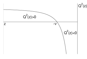
Figure 1: (a) Behavior of the function $Q^{2}(z)$ for $\nu<0$ (b) Contour of integration $\Gamma_{-\nu}(z)$ for $-z<-\nu$. (c) Contour of integration $\Gamma_{-\nu}(z)$ for $-\nu<-z<0$. The dashed line indicates the path of integration on the second Riemann sheet.

Using Eq. (32) we have that the ninth-order approximation ($2N+1=9\rightarrow N=4$) of the function $q(z)$ has the form

$$q(z)=\sum_{n=0}^{4}Y_{2n}Q(z)=\left(Y_{0}+Y_{2}+Y_{4}+Y_{6}+Y_{8}\right)Q(z).$$ (69)

In order to compute $q(z)$ in Eq. (69), we need to compute the coefficients $Y_{2n}$ (26)-(30). The calculation of $Y_{2n}$ requires the knowledge of the coefficients $\epsilon_{\nu}$. Using Eq. (19) and Eq. (31) we obtain

$$\epsilon_{0} =\frac{z^{2}}{\left(z^{2}-\nu^{2}\right)^{3}}\left(\frac{z^{2}}{4}+\nu^{2}\right),$$ (70)

$$\epsilon_{1} =-\frac{z^{2}}{\left(z^{2}-\nu^{2}\right)^{\frac{9}{2}}}\left(\frac{z^{4}}{2}+5\nu^{2}z^{2}+2\nu^{4}\right),$$ (71)

$$\epsilon_{2} =\frac{z^{2}}{\left(z^{2}-\nu^{2}\right)^{6}}\left(\frac{3z^{6}}{2}+28\nu^{2}z^{4}+34\nu^{4}z^{2}+4\nu^{6}\right),$$ (72)

$$\epsilon_{3} =-\frac{z^{2}}{\left(z^{2}-\nu^{2}\right)^{\frac{15}{2}}}\left(6z^{8}+180\nu^{2}z^{6}+440\nu^{4}z^{4}+176\nu^{6}z^{2}+8\nu^{8}\right),$$ (73)

$$\epsilon_{4} =\frac{z^{2}}{\left(z^{2}-\nu^{2}\right)^{9}}\left(30z^{10}+1320\nu^{2}z^{8}+5400\nu^{4}z^{6}+4576\nu^{6}z^{4}+808\nu^{8}z^{2}+16\nu^{10}\right),$$ (74)

$$\epsilon_{5} =-\frac{z^{2}}{\left(z^{2}-\nu^{2}\right)^{\frac{21}{2}}}\left(180z^{12}+10920\nu^{2}z^{10}+67200\nu^{4}z^{8}+98112\nu^{6}z^{6}+38768\nu^{8}z^{4}+\right.$$ (75)

$$\left.+3488\nu^{10}z^{2}+32\nu^{12}\right),$$

$$\epsilon_{6} =\frac{z^{2}}{\left(z^{2}-\nu^{2}\right)^{12}}\left(1260z^{14}+100800\nu^{2}z^{12}+870240\nu^{4}z^{10}+1947456\nu^{6}z^{8}+\right.$$ (76)

$$+\left.1366416\nu^{8}z^{6}+291904\nu^{10}z^{4}+14560\nu^{12}z^{2}+64\nu^{14}\right).$$

Inserting Eq (70)-(76) into Eq. (27)-(30) we obtain that the first four $Y_{2n}$ are

$$Y_{2} =\frac{z^{2}}{\left(z^{2}-\nu^{2}\right)^{3}}\left(\frac{z^{2}}{8}+\frac{\nu^{2}}{2}\right),$$ (77)

$$Y_{4} =-\frac{z^{2}}{\left(z^{2}-\nu^{2}\right)^{6}}\left(\frac{25z^{6}}{128}+\frac{57\nu^{2}z^{4}}{16}+\frac{35\nu^{4}z^{2}}{8}+\frac{\nu^{6}}{2}\right),$$ (78)

$$Y_{6} =\frac{z^{2}}{\left(z^{2}-\nu^{2}\right)^{9}}\left(\frac{1073z^{10}}{1024}+\frac{11171\nu^{2}z^{8}}{256}+\frac{11511\nu^{4}z^{6}}{64}+\frac{611\nu^{6}z^{4}}{4}+\frac{213\nu^{8}z^{2}}{8}+\frac{\nu^{10}}{2}\right),$$ (79)

$$Y_{8} =-\frac{z^{2}}{\left(z^{2}-\nu^{2}\right)^{12}}\left(\frac{375733z^{14}}{32768}+\frac{1752101\nu^{2}z^{12}}{2048}+\frac{7572705\nu^{4}z^{10}}{1024}+\frac{4252813\nu^{6}z^{8}}{256}+\right.$$ (80)

$$\left.+\frac{1491943\nu^{8}z^{6}}{128}+\frac{39561\nu^{10}z^{4}}{16}+\frac{967\nu^{12}z^{2}}{8}+\frac{\nu^{14}}{2}\right).$$

After computing the coefficients $Y_{2n}$ up to $N=4$ we obtain a ninth-order approximation for $q(z)$. The next step is to compute $\omega(z)$. Fig. 1 (b)-(c) show the contours of integration used for computing the integral $\omega(z)$ beginning with the second-order of approximation. Thus we have

$$\omega(z) = w_{0}(z)+\sum_{n=1}^{4}w_{2n}(z),$$ (81)

$$= \int_{-\nu}^{-z}Q(z)dz+\frac{1}{2}\sum_{n=1}^{4}\int_{\Gamma_{-\nu}}Y_{2n}Q(z)dz.$$ (82)

The expressions for $\omega_{2n}(z)$, written in the variable $\eta$, up to $N=4$, are:

$$\omega_{0} =\sqrt{(-k\eta)^{2}-\nu^{2}}-\nu\arccos\frac{\nu}{-k\eta},\quad-k\eta<-\nu,$$ (83)

$$i\omega_{0} =-\sqrt{\nu^{2}-(-k\eta)^{2}}+\nu\ln\left|\frac{\nu+\sqrt{\nu^{2}-(-k\eta)^{2}}}{-k\eta}\right|,\quad-\nu<-k\eta<0,$$ (84)

$$\left.\begin{array}[]{cc}\omega_{2}\\ i\omega_{2}&\end{array}\right\} =\mp\frac{1}{24\left[\pm(-k\eta)^{2}\mp\nu^{2}\right]^{3/2}}\left[2\nu^{2}+3(-k\eta)^{2}\right],$$ (87)

$$\left.\begin{array}[]{cc}\omega_{4}\\ i\omega_{4}&\end{array}\right\} =\frac{1}{5760\left[\pm(-k\eta)^{2}\mp\nu^{2}\right]^{9/2}}\left[375(-k\eta)^{6}+3654\nu^{2}(-k\eta)^{4}+1512\nu^{4}(-k\eta)^{2}-16\nu^{6}\right],$$ (90)

$$\left.\begin{array}[]{cc}\omega_{6}\\ i\omega_{6}&\end{array}\right\} =\mp\frac{1}{322560\left[\pm(-k\eta)^{2}\mp\nu^{2}\right]^{15/2}}\left[67599(-k\eta)^{10}+1914210\nu^{2}(-k\eta)^{8}+\right.$$ (93)

$$\left.+4744640\nu^{4}(-k\eta)^{6}+1891200\nu^{6}(-k\eta)^{4}+78720\nu^{8}(-k\eta)^{2}+256\nu^{10}\right],$$

$$\left.\begin{array}[]{cc}\omega_{8}\\ i\omega_{8}&\end{array}\right\} =\frac{1}{3440640\left[\pm(-k\eta)^{2}\mp\nu^{2}\right]^{21/2}}\left[5635995(-k\eta)^{14}+318291750\nu^{2}(-k\eta)^{12}+\right.$$ (96)

$$+1965889800\nu^{4}(-k\eta)^{10}+2884531440\nu^{6}(-k\eta)^{8}+1135145088\nu^{8}(-k\eta)^{6}+$$

$$\left.+99783936\nu^{10}(-k\eta)^{4}+881664\nu^{12}(-k\eta)^{2}-2048\nu^{14}\right],$$

where the upper and lower expressions on the left side and the upper and lower signs on the right side in (87)-(96) correspond to $-k\eta<-\nu$ and $-\nu<-k\eta<0$ respectively. After computing $\omega(z)$, using the relations (II.1) and (II.1) we obtain a ninth-order phase integral approximation to the solution of the equation for scalar and tensor perturbations (51). The constants $c_{1}$ and $c_{2}$ are computed using the asymptotic behavior of $u_{k}$. We calculate the limit $-k\eta\rightarrow\infty$ of the solution (51) on the left of the turning point (II.1). Choosing $c_{2}=-ic_{1}$ with $c_{1}=e^{i\left(\nu+\frac{1}{2}\right)\frac{\pi}{2}}/\sqrt{2}$ and $c_{2}=e^{i\left(\nu-\frac{1}{2}\right)\frac{\pi}{2}}/\sqrt{2}$, we obtain the asymptotic boundary condition given by Eq. (5). In order to compute the power spectrum we need to evaluate the limit $-k\eta\rightarrow 0$ for the growing part of the solution (II.1). In this limit we have

$$u_{k}^{phi}(\eta)\rightarrow\exp\left[i\left(\nu-\frac{1}{2}\right)\frac{\pi}{2}\right]f^{pi}_{\nu}\frac{1}{\sqrt{k}}\left(-k\eta\right)^{\frac{1}{2}-\nu},$$ (97)

where

$$f^{phi}_{\nu}=\left(2\nu\right)^{\nu-\frac{1}{2}}\exp\left(-\nu+\frac{1}{12\nu}-\frac{1}{360\nu^{3}}+\frac{1}{1260\nu^{5}}-\frac{1}{1680\nu^{7}}\right).$$ (98)

Using Eq. (97), we have that the scalar and tensor spectra, given by Eq. (46) and Eq. (47) are

$$P_{S}^{phi}(k) = \frac{1}{l_{0}^{2}M_{Pl}^{2}}\mathrm{g}^{phi}_{\nu}k^{3-2\nu},$$ (99)

$$P_{T}^{phi}(k) = \frac{1}{l_{0}^{2}}h^{phi}_{\nu}k^{3-2\nu},$$ (100)

where

$$g^{phi}_{\nu} = \left(\frac{1-2\nu}{3-2\nu}\right)\left[\frac{f^{phi}_{\nu}}{2\pi}\right]^{2},$$ (101)

$$h^{phi}_{\nu} = \left[\frac{2^{1/2}f^{phi}_{\nu}}{2\pi}\right]^{2}.$$ (102)

The spectral indices, given by Eq. (48) and Eq. (49) coincide with the exact ones given in Eq. (57) and Eq. (58) respectively. If we only keep the first term, $-\nu$, in the exponential $f^{phi}_{\nu}$ (98), we obtain the first-order phase-integral approximation which coincides with the WKB method after using the Langer modification [4, 3, 5]. If we keep the two first terms in the exponential (98), we obtain the third-order phase integral approximation. It is worth mentioning that, for the power-law model, the tensor and scalar spectral indices do not depend on the order of approximation.

IV Results

In this section we proceed to compare the analytic solutions for the wave function $u_{k}$ and the scalar and power spectra with the results obtained using the phase integral approximation. Fig. 2 compares the real part of the analytic solution of $u_{k}$ with the ninth-order phase integral approximation. The plot is made using the number of e-folds, $N=\ln\ a$, as the independent variable. As expected, the phase integral approximation solution diverges at the root of $q(\eta)$

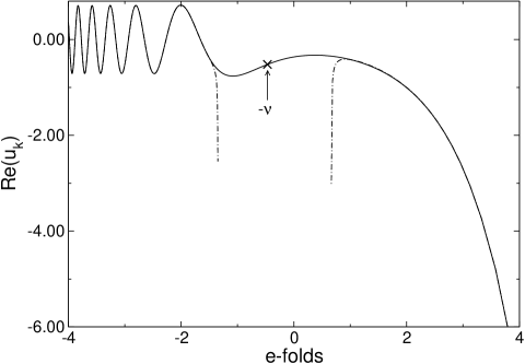
Figure 2: $\Re(u_{k})$ for the power-law inflationary model with $p=10$ with $k=1.389h\mathrm{Mpc}^{-1}$. Solid line: analytic solution; dot-dashed line: ninth-order phase integral approximation.

Now, we compare the scalar and tensor power spectra calculated using the phase-integral approximation with the results obtained with the slow-roll and uniform approximation methods. From Ref. [8] (Eq. (63) and Eq. (64)) we obtain that the scalar and tensor power spectra in the slow-roll approximation are

$$P_{S}^{sr}(k)=\frac{1}{l_{0}^{2}M_{Pl}^{2}}g^{sr}_{\nu}k^{3-2\nu},$$ (103)

$$P_{T}^{sr}(k)=\frac{1}{l_{0}^{2}}h^{sr}_{\nu}k^{3-2\nu},$$ (104)

with

$$g^{sr}_{\nu}=\left[1+2(2-\ln 2+b)(2\epsilon+\delta)-2\epsilon\right]\left(\frac{1-2\nu}{3-2\nu}\right)\left[\frac{2^{-\nu}\left|1-2\nu\right|^{\nu-1/2}}{2\pi}\right]^{2},$$ (105)

$$h^{sr}_{\nu}=\left[1-2(\ln 2+b-1)\epsilon\right]\left[\frac{2^{1/2-\nu}\left|1-2\nu\right|^{\nu-1/2}}{2\pi}\right]^{2},$$ (106)

where b is the Euler constant, $2-\ln 2-b\simeq 0.7296$, $\ln 2+b-1\simeq 0.2704$, and $\epsilon=-\delta=\frac{1}{p}$. In the slow-roll approximation $\epsilon\ll 1$, therefore, for the power-law model, the slow-roll approximation is better suited for large values of the parameter $p$.

Using the result obtained in Ref. [6] (Eq. (109)), we obtain an expression for the second-order uniform approximation for the power spectrum associated with the scalar and tensor perturbations. They have the form:

$$P_{S}^{ua}(k)=\frac{1}{l_{0}^{2}M_{Pl}^{2}}g^{ua}_{\nu}k^{3-2\nu},$$ (107)

$$P_{T}^{ua}(k)=\frac{1}{l_{0}^{2}}h^{ua}_{\nu}k^{3-2\nu},$$ (108)

with

$$g^{ua}_{\nu}=\left(1+\frac{1}{6\nu}\right)\left(\frac{1-2\nu}{3-2\nu}\right)\left[\frac{(2\nu)^{\nu-1/2}e^{-\nu}}{2\pi}\right]^{2},$$ (109)

$$h^{ua}_{\nu}=\left(1+\frac{1}{6\nu}\right)\left[\frac{2^{1/2}(2\nu)^{\nu-1/2}e^{-\nu}}{2\pi}\right]^{2}.$$

Omitting the factor $1/{6\nu}$ in Eq. (109) we obtain the first-order uniform approximation, result that coincides with the first-order phase-integral approximation and the WKB method with the Langer modification [3]. Keeping the second term of the expressions in Eq. (109) one gets the second-order uniform approximation.

We want to compare the analytic expression for the scalar and tensor power spectra for different values of $k$ with the ninth-order phase integral approximation, the slow-roll approximation and the first and second-order uniform approximation. Fig. 3 and Fig. 4 show the power spectra $P_{S}(k)$ and $P_{T}(k)$ calculated analytically as well as with different approximation methods. The inset in each figure represents an enlargement that permits one to compare the accuracy of the different methods. We stop the computation of $P_{S}(k)$ and $P_{T}(k)$ when the quotient $u_{k}/z$ (scalar perturbations) or $u_{k}/a$ (tensor perturbations) becomes constant, i.e., when the function $u_{k}$ leaves the horizon.

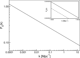
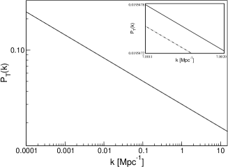
Figure 3: (a) Scalar power spectrum $P_{S}(k)$ and (b) tensor power spectrum $P_{T}(k)$ for the power-law inflationary model with $p=10$. The solid line indicates the analytic solution. The dot-dashed line: ninth-order phase integral approximation. The inset in each figure represents an enlargement that permits one to compare the accuracy of each method.

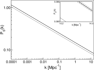
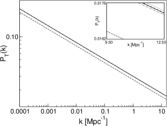
Figure 4: (a) Scalar power spectrum $P_{S}(k)$ and (b) tensor power spectrum $P_{T}(k)$ for the power-law inflationary model with $p=10$. Solid line: Analytic solution; dotted line: slow-roll approximation; dashed line: first-order phase-integral approximation, WKB and first-order uniform approximation; dot-dashed line: third-order phase integral approximation; dot-dot-dashed line: second-order uniform approximation. The inset in each figure represents an enlargement that permits one to compare the accuracy of each method.

Fig. 5 shows the quotient between the exact analytic result and the result obtained using different methods of approximation $g^{\mathrm{j}}_{p}/g^{\mathrm{ex}}_{p}$ for different values of $p$. Using the ninth-order phase integral approximation we obtain a horizontal line equal to unity. We observe analogous behavior when we consider the quotient $h^{\mathrm{j}}_{p}/h^{\mathrm{ex}}_{p}$. As it was already mentioned, the slow-roll approximation is better suited for large values of $p$ because $\epsilon=1/p$. The WKB method gives a better approximation for small values of $p$ because the condition $\mu\ll 1$ is valid in this case. It should be noticed that the first-order phase-integral approximation, the WKB method with the Langer modification and the first-order uniform approximation give the same result.

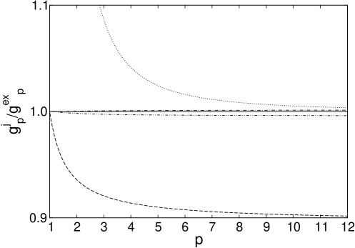
Figure 5: Evolution of the ratio $g^{j}(p)/g^{ex}(p)$ versus $p$. Solid line: ninth-order phase integral approximation; dotted line: slow-roll approximation; dashed line: first-order phase integral, WKB and first-order uniform approximations; dot-dashed line: third-order phase-integral approximation; dot-dot-dashed line: second-order uniform approximation.

Fig.6 and Fig.6 show, the relative error of $P_{\mathrm{S}}(k)$ and $P_{\mathrm{T}}(k)$ respectively for different approximation methods. The relative error is computed using the following expression:

$$\text{rel. error}\,\,P_{{\mathrm{S}},{\mathrm{T}}}(k)=\frac{\left[P_{{\mathrm{S}},{\mathrm{T}}}^{\text{\text{approx}}}(k)-P_{{\mathrm{S}},{\mathrm{T}}}^{\mathrm{ex}}(k)\right]}{P_{{\mathrm{S}},{\mathrm{T}}}^{\mathrm{ex}}(k)}\times 100.$$ (110)

Approximation	$\left|\text{rel. error}\,\,P_{\mathrm{S}}(k)\right|$	$\left|\text{rel. error}\,\,P_{\mathrm{T}}(k)\right|$
phi9${}^{\text{\tiny{a}}}$	$0.0015\%$	$0.0015\%$
phi3${}^{\text{\tiny{b}}}$	$0.1\%$	$0.1\%$
ua2${}^{\text{\tiny{c}}}$	$0.4\%$	$0.4\%$
sr${}^{\text{\tiny{d}}}$	$0.5\%$	$0.5\%$
phi1${}^{\text{\tiny{e}}}$, $\textnormal{WKB}_{\mathrm{LM}}^{\text{\tiny{f}}}$, ua1${}^{\text{\tiny{g}}}$	$10\%$	$10\%$

Table 1: Relative error obtained using different methods of approximation for the power-law inflationary model with $p=10$ for the mode $k=1.369\,h\,{\mathrm{Mpc}}^{-1}$.

${}^{\text{\tiny{a}}}$Ninth-order phase integral approximation.

${}^{\text{\tiny{b}}}$Third-order phase integral approximation.

${}^{\text{\tiny{c}}}$Second-order uniform approximation.

${}^{\text{\tiny{d}}}$Slow-roll approximation.

${}^{\text{\tiny{e}}}$First-order phase integral approximation.

${}^{\text{\tiny{f}}}$ WKB approximation with the Langer modification.

${}^{\text{\tiny{g}}}$First-order uniform approximation.

Table 1 shows that the ninth-order phase integral approximation gives the smallest relative error for $P_{\mathrm{S}}(k)$ and $P_{\mathrm{T}}(k)$. The third-order phase integral approximation gives a relative error smaller than the one obtained using the second-order uniform approximation.

Finally, some words about the accuracy of the phase-integral approximation are in order: The smallness of the integral $\mu(z,z_{0})$ given by Eq. (36) is a measure of the accuracy of the phase-integral approximation. Fig. 2 shows that the phase-integral method fails in the vicinity of the turning point $-\nu$, range where the $\mu$-integral diverges. The selection of the base function $Q(z)$ given by Eq. (66) guarantees that $\mu\ll 1$ far from the turning point at any order of approximation. Since the scalar and tensor power spectra as well as the spectral indices are evaluated as $-k\eta\rightarrow 0$, the limit is taken far from the horizon (turning point), therefore their computation is not affected by the presence of the turning point. For $p=10$ and $k=1.369hMpc^{-1}$ the turning point is $\nu=-1.61M_{Pl}^{-1}$, and the power spectrum is evaluated at $k\eta=-10^{-8}M_{Pl}^{-1}$, a point in the limit where the function $u_{k}$ exhibits the asymptotic behavior (6). Fig.3, Fig. 4 and Table 1 show the accuracy of the phase-integral approximation.

In the present paper we have shown that, in comparison with other approximation methods, the phase integral approach gives very good results for the scalar and tensor spectra in the power-law inflationary model. We have also seen that the phase integral approach reproduces the exact spectral indices in the power-law model. Since the WKB method can be regarded as a first-order approximation of the phase-integral approximation with $Q^{2}(z)=R(z)$, it should be expected that the phase-integral method works in those cases where the WKB methods gives good estimates and slow-roll fails, that is the case where inflation is generated by a chaotic potential with a step [23]. The good agreement between the analytic results and the phase-integral approximation shows that the phase integral method is a very useful tool for computing the scalar and tensor power spectra in more realistic inflationary scenarios, in a forthcoming work we will implement the phase integral method to quadratic and quartic chaotic models.

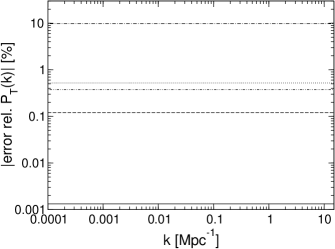
Figure 6: (a) Relative error of $P_{\mathrm{S}}(k)$ and (b) relative error of $P_{\mathrm{T}}(k)$ for the power-law inflationary model with $p=10$. Solid line: ninth-order phase integral approximation, dashed line: third-order phase integral approximation; dot-dot-dashed line: second-order uniform approximation; dotted line : slow roll approximation; dot-dashed line: first-order phase integral approximation, WKB, and first-order uniform approximation

References

[1] D. N. Spergel, R. Bean, O. Doré, M. R. Nolta, C. L. Bennett,
G. Hinshaw, N. Jarosik, E. Komatsu, L. Page, H. V. Peiris, L. Verde,
C. Barnes, M. Halpern, R. S. Hill, A. Kogut, M. Limon, S. S. Meyer,
N. Odegard, G. S. Tucker, J. L. Weiland, E. Wollack, and E. L.
Wright Wilkinson Microwave Anisotropy Probe (WMAP) Three
Year Results: Implications for Cosmology,
http://arxiv.org/abs/astro-ph/0603449
[2]
E. D. Stewart and D. H. Lyth, Phys. Lett. B 302, 171
(1993).
[3]
J. Martin and D. J. Schwarz, Phys. Rev. D 67, 083512
(2003).
[4]
R. Langer, Phys. Rev. 51, 669 (1937).
[5] R. Casadio, F. Finelli, M. Luzzi, and G.
Venturi, Phys. Rev. D 71, 043517 (2005).
[6]
S. Habib, A. Heinen, K. Heitmann, G. Jungman, and C. Molina-París,
Phys. Rev. D, 70 083507, (2004).
[7]
S. Habib, K. Heitmann, G. Jungman, and C. Molina-París, Phys.
Rev. Lett. 89, 281301 (2002).
[8]
S. Habib, A. Heinen, K. Heitmann, and G. Jungman, Phys. Rev. D.
71, 043518 (2005).
[9]
N. Fröman and P. O. Fröman, JWKB Approximation.
Contribution to the Theory (North-Holland, Amsterdam, 1965).
[10] N. Fröman and P.O. Fröman,
Phase-Integral Method. Allowing Nearlying Transition Points,
volume 40. (Springer Tracts in Natural Philosophy, 1996).
[11]
N. Fröman and P. O. Fröman. Physical Problems Solved by the
Phase-Integral Method (Cambridge University Press, 2002).
[12] N. Anderson, M. E. Araujo, and B. F. Schutz, Class.
Quantum Grav. 10, 735 (1993)
[13]K. K Kokkotas and B. Schmidt, Living. Rev.
Relativity http://www.livingreviews.org/lrr-1999-2 (1999).
[14] V. F. Mukhanov, H. A. Feldman, and R. H.
Brandenberger, Phys. Rep. 215, 203 (1992).
[15]
A. R. Liddle and D. H. Lyth. Cosmological Inflation and
Large-Scale Structure. (Cambridge University Press, 2000).
[16] E. Lidsey, A. R. Liddle, E. W. Kolb, E. J.
Copeland, T. Barreiro, and M. Abney Rev. Mod. Phys. 69, 373
(1997).
[17]
N. Fröman, Ark. Fys. 32, 541 (1966).
[18]
N. Fröman and P.O. Fröman, Ann. Phys. 83, 103 (1974).
[19]
J. A. Campbell, J. Comp. Phys. 10, 308 (1972).
[20]
N. Fröman, Ann. Phys. 61, 451 (1970).
[21] L. F. Abbott, Nuc. Phys. B 244, 541 (1984).
[22]
F. Lucchin and S. Matarrese, Phys. Rev. D 32, 1316 (1985).
[23] P. Hunt and S. Sarkar, Phys. Rev. D. 70 103518
(2004).