Light Propagation and Large-Scale Inhomogeneities

Abstract

We consider the effect on the propagation of light of inhomogeneities with sizes of order 10 Mpc or larger. The Universe is approximated through a variation of the Swiss-cheese model. The spherical inhomogeneities are void-like, with central underdensities surrounded by compensating overdense shells. We study the propagation of light in this background, assuming that the source and the observer occupy random positions, so that each beam travels through several inhomogeneities at random angles. The distribution of luminosity distances for sources with the same redshift is asymmetric, with a peak at a value larger than the average one. The width of the distribution and the location of the maximum increase with increasing redshift and length scale of the inhomogeneities. We compute the induced dispersion and bias on cosmological parameters derived from the supernova data. They are too small to explain the perceived acceleration without dark energy, even when the length scale of the inhomogeneities is comparable to the horizon distance. Moreover, the dispersion and bias induced by gravitational lensing at the scales of galaxies or clusters of galaxies are larger by at least an order of magnitude.

1 Introduction

The observed deviation from homogeneity of the structure of the Universe at small length scales poses the question of whether the use of the Friedmann-Robertson-Walker (FRW) metric is adequate for the discussion of the cosmological expansion. The argument for the applicability of a homogeneous solution is based on the observation that the matter distribution is homogeneous when averaged over length scales of ${\cal O}(100)\,h^{-1}$ Mpc. On the other hand, the conclusion drawn from observations of distant supernova [1, 2], or the perturbations of the cosmic microwave background (CMB) [3], that the recent cosmological expansion is accelerating has placed the effect of structure formation on the overall expansion under scrutiny.

We are interested in the influence of inhomogeneities with sub-horizon characteristic scales on the perceived expansion [4, 5, 6]. The observed inhomogeneities in the matter distribution with length scales of ${\cal O}(10)\,h^{-1}$ Mpc or smaller are large, so that the Universe cannot be approximated as homogeneous at these scales. It is important to have a quantitative estimate of the influence of these inhomogeneities on the data used for the determination of the expansion rate. As all the observations involve the detection of light signals, it is crucial to understand the effect of the inhomogeneous background on light propagation.

The transmission of a light beam in a general gravitational background can be studied through the Sachs optical equations [7]. These describe the expansion and shear of the beam along its null trajectory. Apart from the case of a FRW background, the optical equations have been derived by Kantowski for a Scharzschild background [8]. He used them for the study of light transmission within the Swiss-cheese model of the Universe [9]. In this model the light propagates essentially in empty space with a beam expansion larger than the average. In rare instances it passes near a very dense clump of matter, which produces significant shear and focusing of the beam [10]. Because of the randomness of such events, sources with the same intrinsic luminosity and redshift may have different luminosity distances. The distribution is peaked at a value of the luminosity distance larger than the one in a homogeneous background [11, 12], even though the mean value remains unaffected. If the sample of observed sources is small, it unlikely that a clump of matter will be encountered during the beam propagation. The beams essentially propagate in empty space, while the expansion is induced by the average energy density. A phenomenological equation has been proposed by Dyer and Roeder in order to describe the case in which a fraction of the energy density is homogeneously distributed while the remaining is in clumps that do not affect the light propagation [13].

The picture of the Universe we described above is applicable to length scales of ${\cal O}(1)\,h^{-1}$ Mpc or smaller, for which the dominant structures are galaxies or clusters of galaxies. At larger distances the averaged matter distribution has a smaller density contrast. The use of the Schwarzschild geometry for the description of the inhomogeneities is not appropriate. The Lemaitre-Tolman-Bondi (LTB) metric [14] has been employed often for the modelling of the Universe at scales of ${\cal O}(10)\,h^{-1}$ Mpc or larger [15]–[24]. Its use demonstrates that inhomogeneities can induce deviations of the luminosity distance from its value in a homogeneous background. For example, it has been observed that any form of the luminosity distance as a function of redshift can be reproduced with the LTB metric [15]. This means that the supernova data can be explained through an inhomogeneous matter distribution in the context of this metric. However, reproducing the data requires a variation of the density or the expansion rate over distances of ${\cal O}(100)\,h^{-1}$ Mpc or even larger [20]–[24]. In order to avoid a conflict with the isotropy of the CMB the location of the observer must be within a distance of ${\cal O}(10)\,h^{-1}$ Mpc from the center of the spherical configuration described by the LTB metric. In this sense, the explanation of the perceived acceleration relies on the position of the observer. On the other hand, there are indications for the presence of a very large void in our vicinity [25, 26].

Our work is based on the fundamental assumption that we do not occupy a special position in the Universe. We are interested in determining the maximum effect that large-scale inhomogeneities can have on the luminosity distance. The density contrast of inhomogeneities with characteristics lengths of ${\cal O}(10)\,h^{-1}$ Mpc or larger is at most of ${\cal O}(1)$. For this reason it seems unlikely that they can affect the propagation of light more strongly than the inhomogeneities with lengths of ${\cal O}(1)\,h^{-1}$ Mpc or smaller, whose density contrast can be larger than 1 by several orders of magnitude. On the other hand, the validity of the FRW metric is questionable if inhomogeneities with lengths comparable to the horizon distance $\sim 3\times 10^{3}\,h^{-1}$ Mpc develop a density contrast of ${\cal O}(1)$. We shall allow for such a possibility in order to obtain a quantitative estimate of the effect on the luminosity distance.

In a previous publication [27] we derived the optical equations for a general LTB background [14]. We used them in order to study light propagation in a variant of the Swiss-cheese model. The inhomogeneities are modelled as spherical regions within which the geometry is described by the LTB metric. At the boundary of these regions the LTB metric is matched with the FRW metric that describes the evolution in the region between the inhomogeneities. The Universe consists of collapsing or expanding inhomogeneous regions, while a common scale factor exists that describes the expansion of the homogeneous intermediate regions. This model is similar to the standard Swiss-cheese model [9], with the replacement of the Schwarzschild metric with the LTB one. For this reason we refer to it as the LTB Swiss-cheese model.

We focus on the effect of inhomogeneities on the luminosity distance if the source and the observer do not occupy special positions in the Universe. This is achieved by placing both the source and the observer within the homogeneous region of the LTB Swiss-cheese model. During its path the light signal crosses several inhomogeneous regions before reaching the observer. As we have mentioned, similar studies [11, 12] have discussed the influence of structures such as galaxies or clusters of galaxies on light propagation. The beam shear plays an important role in this effect, characterized as gravitational lensing [28]. We focus on inhomogeneities of much larger length scale, of ${\cal O}(10)\,h^{-1}$ Mpc or larger. The matter distribution, even though inhomogeneous, is more evenly distributed than in the previous case. In particular, we assume that each spherical region has a central underdensity surrounded by an overdense shell. The densities in the two regions are comparable at early times and differ by a factor ${\cal O}(1)$ during the later stages of the evolution. The LTB Swiss-cheese model we construct in this way describes a Universe dominated by spherical voids with the compensating matter concentrated in shells surrounding them. The beam shear is negligible in our calculations, and the main effect arises from the variations of the beam expansion because of the inhomogeneities.

In ref. [27] we estimated the deviations of the luminosity distance from its value in a homogeneous Universe by considering the extreme case in which the light passes through the centers of all the inhomogeneities it encounters. In this work we perform a more detailed statistical analysis, by considering light beams with random impact parameters relative to the centers. We check that the resulting luminosity distance as a function of the impact parameter is consistent with flux conservation. For a given redshift we estimate the width of the distribution of luminosity distances. We also determine the deviation of the maximum of the distribution from the value in a homogeneous background. For a central underdensity this value is positive and sets the scale for the perceived increase in the expansion rate relative to a homogeneous Universe. An analytical study with similarities with our work is described in ref. [29]. It focuses, however, on the study of the redshift, which determines only partially the luminosity distance. No statistical analysis, which is the central point of our work, is performed either.

In the following section we summarize the geodesic and optical equations in a LTB background. In section 3 we describe the cosmological evolution of the inhomogeneous regions. In section 4 we study, both numerically and analytically, the effect of the inhomogeneity on the properties (redshift,beam area) of a light beam that travels through it. In section 5 we study the luminosity distance as a function of the angle at which the beam crosses the inhomogeneity. We verify that the results are consistent with flux conservation. In section 6 we consider multiple crossings of inhomogeneities by the light beam and the effect on the luminosity distance. We calculate the distribution of the deviations of the luminosity distance from its value in a homogeneous background. In section 7 we estimate the effect on the determination of cosmological parameters from supernova data.

2 Luminosity distance in a Lemaitre-Tolman-Bondi (LTB) background

Under the assumption of spherical symmetry, the most general metric for a pressureless, inhomogeneous fluid is the LTB metric [14]. It can be written in the form

$$ds^{2}=-dt^{2}+b^{2}(t,r)dr^{2}+R^{2}(t,r)d\Omega^{2},$$ (2.1)

where $d\Omega^{2}$ is the metric on a two-sphere. The function $b(t,r)$ is given by

$$b^{2}(t,r)=\frac{R^{\prime 2}(t,r)}{1+f(r)},$$ (2.2)

where the prime denotes differentiation with respect to $r$, and $f(r)$ is an arbitrary function. The bulk energy momentum tensor has the form

$$T^{A}_{~{}B}={\rm diag}\left(-\rho(t,r),\,0,\,0,\,0\right).$$ (2.3)

The fluid consists of successive shells marked by $r$, whose local density $\rho$ is time-dependent. The function $R(t,r)$ describes the location of the shell marked by $r$ at the time $t$. Through an appropriate rescaling it can be chosen to satisfy $R(0,r)=r$.

The Einstein equations reduce to

$$\dot{R}^{2}(t,r) = \frac{1}{8\pi M^{2}}\frac{{\cal M}(r)}{R}+f(r)$$ (2.4)

$${\cal M}^{\prime}(r) = 4\pi R^{2}\rho\,R^{\prime},$$ (2.5)

where the dot denotes differentiation with respect to $t$, and $G=\left(16\pi M^{2}\right)^{-1}$. The generalized mass function ${\cal M}(r)$ of the fluid can be chosen arbitrarily. Because of energy conservation ${\cal M}(r)$ is independent of $t$, while $\rho$ and $R$ depend on both $t$ and $r$.

Without loss of generality we consider geodesic null curves on the plane with $\theta=\pi/2$. The first geodesic equation is

$$\frac{dk^{0}}{d\lambda}+\frac{\dot{R}^{\prime}R^{\prime}}{1+f}\left(k^{1}\right)^{2}+\dot{R}R\left(k^{3}\right)^{2}=0,$$ (2.6)

with $k^{i}={dx^{i}}/{d\lambda}$ and $\lambda$ an affine parameter along the null beam trajectory. The second geodesic equation can be replaced by the null condition

$$-\left(k^{0}\right)^{2}+\frac{R^{\prime 2}}{1+f}\left(k^{1}\right)^{2}+R^{2}\left(k^{3}\right)^{2}=0,$$ (2.7)

while the third one can be integrated to obtain

$$k^{3}=\frac{c_{\phi}}{R^{2}}.$$ (2.8)

The equation for the beam area can be written as [27]

$$\frac{1}{\sqrt{A}}\frac{d^{2}\sqrt{A}}{d\lambda^{2}}=-\frac{1}{4M^{2}}\rho\left(k^{0}\right)^{2}-\sigma^{2}.$$ (2.9)

The shear $\sigma$ is generated by inhomogeneities, for which the local energy density is different from the average one [27]. It describes the deformations of the cross-section of the beam, induced by the propagation within an inhomogeneous medium. The shear is important when the beam passes near regions in which the density exceeds the average one by several orders of magnitude. Within our modelling of large-scale structure, applicable for scales above ${\cal O}(10)\,h^{-1}$ Mpc, the average density contrast is not sufficiently large for the shear to become important. (We have verified this conclusion numerically.) For this reason we neglect it in our study.

The Friedmann-Robertson-Walker (FRW) metric is a special case of the LTB metric with

$$R(t,r)=a(t)r~{}~{}~{}~{}~{}~{}~{}~{}~{}~{}~{}~{}~{}~{}~{}f(r)=cr^{2},~{}~{}~{}c=0,\pm 1$$ (2.10)

$$\rho=\frac{c_{\rho}}{a^{3}(t)}~{}~{}~{}~{}~{}~{}~{}~{}~{}~{}~{}~{}~{}~{}~{}~{}~{}~{}~{}~{}~{}~{}~{}{\cal M}(r)=\frac{4\pi}{3}c_{\rho}r^{3}.$$ (2.11)

The geodesic equation (2.6) has the solution

$$k^{0}=\frac{c_{t}}{a(t)}.$$ (2.12)

The solution of eq. (2.9) for an outgoing beam is

$$A(\lambda)=r^{2}(\lambda)\,a^{2}(t(\lambda))\,\Omega_{s}.$$ (2.13)

If we normalize the scale factor so that $a(t_{s})=1$ at the time of the beam emission, we recover the standard expression $A=r^{2}\Omega_{s}$ in flat space-time. The constant $\Omega_{s}$ can be identified with the solid angle spanned by a certain beam when the light is emitted by a point-like isotropic source. We are interested in light propagation in more general backgrounds. We assume that the light emission near the source is not affected by the large-scale geometry. By choosing an affine parameter that is locally $\lambda=t$ in the vicinity of the source, we can set

$$\left.\frac{d\sqrt{A}}{d\lambda}\right|_{\lambda=0}=\sqrt{\Omega_{s}}.$$ (2.14)

This expression, along with

$$\left.\sqrt{A}\right|_{\lambda=0}=0,$$ (2.15)

provide the initial conditions for the solution of eq. (2.9).

In order to define the luminosity distance, we consider photons emitted within a solid angle $\Omega_{s}$ by an isotropic source with luminosity $L$. These photons are detected by an observer for whom the light beam has a cross-section $A_{o}$. The redshift factor is

$$1+z=\frac{\omega_{s}}{\omega_{o}}=\frac{k^{0}_{s}}{k^{0}_{o}},$$ (2.16)

because the frequencies measured at the source and at the observation point are proportional to the values of $k^{0}$ at these points. The energy flux $f_{o}$ measured by the observer is

$$f_{o}=\frac{L}{4\pi D_{L}^{2}}=\frac{L}{4\pi}\frac{\Omega_{s}}{(1+z)^{2}A_{o}}.$$ (2.17)

The above expression allows the determination of the luminosity distance $D_{L}$ as a function of the redshift $z$. The beam area can be calculated by solving eq. (2.9), with initial conditions given by eqs. (2.14), (2.15), while the redshift is given by eq. (2.16).

3 Modelling the inhomogeneities

We study the effect of inhomogeneities on the luminosity distance without assuming a preferred location of the observer. We model the inhomogeneities as spherical regions within which the geometry is described by the LTB metric. At the boundary of these regions, the LTB metric is matched with the FRW metric that describes the expansion of the homogeneous intermediate regions. Our model is similar to the standard Swiss-cheese model [9], with the replacement of the Schwarzschild metric with the LTB one. For this reason we refer to it as the LTB Swiss-cheese model.

The choice of the two arbitrary functions ${\cal M}(r)$ and $f(r)$ in eq. (2.1) can lead to different physical situations. The mass function ${\cal M}(r)$ is related to the initial matter distribution. The function $f(r)$ defines an effective curvature term in eq. (2.4). We work in a gauge in which $R(0,r)=r$. We parametrize the initial energy density as $\rho_{i}(r)=\left(1+\epsilon(r)\right)\rho_{0,i}$, with $\rho_{i}(r)=\rho(0,r)$ and $|\epsilon(r)|<1$. The initial energy density of the homogeneous background is $\rho_{0,i}$. If the size of the inhomogeneity is $r_{0}$, a consistent solution requires $4\pi\int_{0}^{r_{0}}r^{2}\epsilon(r)dr=0$, so that

$${\cal M}(r_{0})=4\pi\int_{0}^{r_{0}}r^{2}\rho(r)\,dr=\frac{4\pi}{3}r^{3}_{0}\rho_{0,i}.$$ (3.1)

This is obvious if we apply eqs. (2.4), (2.5) to the homogeneous part at $r>r_{0}$. The FRW metric is a special case of the LTB metric, described by eqs. (2.10), (2.11). Consistency of the equations as the shell with $r=r_{0}$ is approached from both sides imposes the condition (3.1). Moreover, the absence of singularities requires the continuity of $f(r)$ and $f^{\prime}(r)$. As we assume that the homogeneous part is flat, this means that $f(r_{0})=f^{\prime}(r_{0})=0$. Alternatively, one may consider the matching of the two metrics at the surface with $r=r_{0}$ employing junction conditions [30]. If this surface does not contain a singular energy density, the above constraints must be imposed [29, 31].

We assume that at the initial time $t_{i}=0$ the expansion rate $H_{i}=\dot{R}/R=\dot{R}^{\prime}/R^{\prime}$ is given for all $r$ by the standard expression in homogeneous cosmology: $H_{i}^{2}=\rho_{0,i}/(6M^{2})$. Then, eq. (2.4) with $R(0,r)=r$ implies that

$$f(r)=\frac{\rho_{0,i}}{6M^{2}}r^{2}\left(1-\frac{3{\cal M}(r)}{4\pi r^{3}\rho_{0,i}}\right).$$ (3.2)

The spatial curvature of the LTB geometry is

$${}^{(3)}R(r,t)=-2\frac{(fR)^{\prime}}{R^{2}R^{\prime}}.$$ (3.3)

For our choice of $f(r)$ we find that at the initial time

$${}^{(3)}R(r,0)=-6H^{2}_{i}\left(1-\frac{{\cal M}^{\prime}}{4\pi r^{2}\rho_{0,i}}\right)=-6H^{2}_{i}\left(1-\frac{\rho_{i}(r)}{\rho_{0,i}}\right).$$ (3.4)

Overdense regions have positive spatial curvature, while underdense ones negative curvature. This is very similar to the initial condition considered in the model of spherical collapse [32].

When the inhomogeneity is denser near the center, we have $f(r)<0$ for $r<r_{0}$ and $f(r)=0$ for $r\geq r_{0}$. It is then clear from eq. (2.4) that, in an expanding Universe, the central region will have $\dot{R}=0$ at some point in its evolution and will stop expanding. Subsequently, it will reverse its motion and start collapsing. The opposite happens if the inhomogeneity has a central underdensity. In this case, the central region expands faster than the surrounding denser spherical shell. The width of the shell decreases, while its density increases. It is the latter configuration that is relevant if we want to model the Universe as being composed mainly of voids separated by thin dense regions.

Our expressions simplify if we switch to dimensionless variables. We define ${\bar{t}}=tH_{i}$, ${\bar{r}}=r/r_{0}$, ${\bar{R}}=R/r_{0}$, where $H^{2}_{i}=\rho_{0,i}/(6M^{2})$ is the initial homogeneous expansion rate and $r_{0}$ gives the size of the inhomogeneity in comoving coordinates. The evolution equation becomes

$$\frac{\dot{{\bar{R}}}^{2}}{{\bar{R}}^{2}}=\frac{3{\bar{\cal M}}({\bar{r}})}{4\pi{\bar{R}}^{3}}+\frac{{\bar{f}}({\bar{r}})}{{\bar{R}}^{2}},$$ (3.5)

with $\bar{{\cal M}}={\cal M}/(\rho_{0,i}r^{3}_{0})$ and ${\bar{f}}=6M^{2}f/(\rho_{0,i}r_{0}^{2})=f/{\bar{H}}^{2}_{i}$, ${\bar{H}}_{i}=H_{i}r_{0}$. The dot now denotes a derivative with respect to ${\bar{t}}$.

We take the affine parameter $\lambda$ to have the dimension of time and we define the dimensionless variables ${\bar{\lambda}}=H_{i}\lambda$, $\bar{k}^{0}=k^{0}$, $\bar{k}^{1}=k^{1}/{\bar{H}}_{i}$, $\bar{k}^{3}=r_{0}k^{3}$. The geodesic equations (2.6)–(2.8) maintain their form, with the various quantities replaced by barred ones, and the combination $1+f$ replaced by ${\bar{H}}_{i}^{-2}+{\bar{f}}$. For geodesics going through subhorizon perturbations with ${\bar{H}}_{i}\ll 1$ the effective curvature term ${\bar{f}}$ plays a minor role. However, this term is always important for the evolution of the perturbations, as can be seen from eq. (3.5). The optical equation takes the form

$$\frac{1}{\sqrt{{\bar{A}}}}\frac{d^{2}\sqrt{{\bar{A}}}}{d{\bar{\lambda}}^{2}}=-\frac{3}{2}\bar{\rho}\left(\bar{k}^{0}\right)^{2},$$ (3.6)

with $\bar{\rho}=\rho/\rho_{0,i}$. We omitted the shear, as it gives a negligible contribution to our results. The initial conditions (2.14), (2.15) become

$$\left.\frac{d\sqrt{{\bar{A}}}}{d{\bar{\lambda}}}\right|_{{\bar{\lambda}}=0}=\frac{1}{{\bar{H}}_{i}}\sqrt{{\bar{\Omega}}_{s}}=\sqrt{\Omega_{s}}.$$ (3.7)

$$\left.\sqrt{{\bar{A}}}\right|_{\lambda=0}=0,$$ (3.8)

with ${\bar{A}}=H_{i}^{2}A$ and ${\bar{\Omega}}={\bar{H}}_{i}^{2}\Omega$.

Figure 1: The evolution of the density profile for a central underdensity surrounded by an overdensity.

4 Single crossing

The typical cosmological evolution is displayed in fig. 1 for a central underdensity that is surrounded by an overdense region. The initial density $\bar{\rho}_{i}(r)=\rho_{i}(r)/\rho_{0,i}=1+\epsilon(r)$ is constant $\bar{\rho}_{i}=1+\epsilon_{1}$ in the region ${\bar{r}}\leq 0.8$, constant $\bar{\rho}_{i}=1+\epsilon_{2}$ in the region $0.9\leq{\bar{r}}\leq 0.95$, and $\bar{\rho}_{i}=1$ for ${\bar{r}}\geq 1$. In the intervals $0.8\leq{\bar{r}}\leq 0.9$ and $0.95\leq{\bar{r}}\leq 1$ it interpolates linearly between the values at the boundaries. This guarantees that the conditions ${\bar{f}}(1)={\bar{f}}^{\prime}(1)=0$, imposed by the matching of the FRW and LTB metrics, are satisfied. We use $\epsilon_{1}=-0.01$. The value of $\epsilon_{2}$ is fixed by the requirement that $\int_{0}^{1}\epsilon({\bar{r}}){\bar{r}}^{2}d{\bar{r}}=0$. In a previous publication [27], we studied in detail the evolution of such inhomogeneities. We showed analytically that their growth is consistent with the standard theory of structure formation and the spherical collapse model [32]. Inhomogeneities that are initially of horizon size (${\bar{H}}_{i}\sim 1$) with $|\epsilon_{1}|\sim 10^{-5}$ and have a characteristic scale ${\cal O}(10)\,h^{-1}$ Mpc today also have a density contrast of ${\cal O}(1)$. In our numerical solutions we do not follow the very early evolution of the inhomogeneities. The perturbations we consider are already of subhorizon size and have a density contrast of ${\cal O}(10^{-2})$. They evolve to form present-day structures with size ${\cal O}(10)\,h^{-1}$ Mpc or larger and density contrast of ${\cal O}(1)$. The profile of the perturbations that we assume in this work differs slightly from the one in ref. [27] with respect to the width of the shell. In ref. [27] the widths of the underdense and overdense regions were taken equal. In this work we assume that the initial shells are narrower and denser than in ref. [27]. Clearly, our modelling of the Universe cannot reproduce all the details of the statistical nature of the inhomogeneities, especially during their evolution in the non-linear regime. Our choice results in a model of the Universe dominated by voids, in rough agreement with observations. It is possible, however, that the effect of underdensities is overestimated, as they occupy a slightly larger fraction of the total volume than the overdense regions already in the initial small perturbations.

In fig. 1 we display the density profile at times ${\bar{t}}$=10, 100, 200, 250. We follow the evolution at later times as well, even though we do not depict it in fig. 1. We normalize the energy density to that of a homogenous FRW background (given by $\bar{\rho}_{FRW}({\bar{t}})=\bar{\rho}({\bar{t}},1)$). The earliest time corresponds to the curve with the smallest deviation from 1, while the latest to the curve with the largest deviation. We observe that the density contrast grows and eventually becomes of ${\cal O}(1)$. The central energy density drops relative to the homogeneous background, while the surrounding region becomes denser. The radius of the central underdensity grows relative to the total size of the inhomogeneity, as this region expands faster than the average. The surrounding shell becomes thinner and denser.

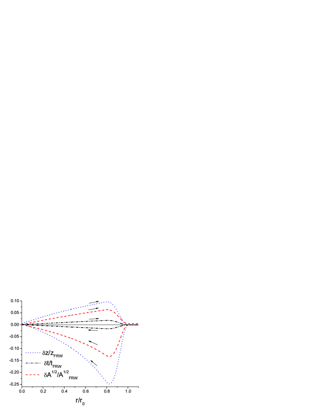
Figure 2: The relative difference in redshift, coordinate time, and beam area, between the propagation in the background of fig. 1 and in a homogeneous background, as a function of the radial coordinate.

The effect of the spherical inhomogeneity on the characteristics of a light beam is depicted in figs. 2, 3. (Fig. 3 is a magnification of fig. 2 around ${\bar{r}}=0$.) We assume a perturbation with ${\bar{H}}_{i}=1$ at the initial time ${\bar{t}}_{i}=0$, so that the effects on the light beam are clearly visible. We use this perturbation for the numerical analysis both in this section and in section 5. Such a perturbation leads to an inhomogeneity at the present time with size that would be in conflict with observations (approximately $350\,h^{-1}$ Mpc). We consider realistic perturbations in section 6. We consider a beam with $c_{\phi}=0$ that is emitted from a point with ${\bar{r}}_{s}=1.5$ and passes through the center of symmetry. The emission time is ${\bar{t}}_{s}=250$ and the signal reaches ${\bar{r}}=1.5$ again at a time ${\bar{t}}\simeq 441$. The redshift for the exiting beam at ${\bar{r}}=1.5$ is $z\simeq 0.46$. We plot the relative difference in redshift $(z-z_{FRW})/z_{FRW}$, coordinate time $({\bar{t}}-{\bar{t}}_{FRW})/{\bar{t}}_{FRW}$, and beam area $\left(\sqrt{{\bar{A}}}-\sqrt{{\bar{A}}_{FRW}}\right)/\sqrt{{\bar{A}}_{FRW}}$, between the propagation in the background of fig. 1 and in a homogeneous background, as a function of the radial coordinate ${\bar{r}}$. The arrows indicate the evolution of various quantities as the beam enters the inhomogeneity from one side and exits from the other. In the region $0.1\mathrel{\vbox{\hbox{$<$}\nointerlineskip\hbox{$\sim$}}}{\bar{r}}\mathrel{\vbox{\hbox{$<$}\nointerlineskip\hbox{$\sim$}}}0.9$ we observe a significant deviation of all quantities from their values in a homogeneous background. However, the deviation becomes small in the region near the origin. When the beam moves out of the inhomogeneous region only the beam area deviates from the value in a homogeneous background. The coordinate time and the redshift are not affected significantly.

We can obtain an understanding of the evolution depicted in figs. 2, 3 through an analytical treatment. The effect of the inhomogeneity on the characteristics of the light beam can be estimated analytically for perturbations with size much smaller than the distance to the horizon. These have ${\bar{H}}_{i}\ll 1$. Let us consider a beam with $c_{\phi}=0$ that passes through the center of the spherical inhomogeneity. The null condition (2.7) can be written as

$$\frac{d{\bar{t}}}{d{\bar{r}}}=\mp{\bar{H}}_{i}\frac{{\bar{R}}^{\prime}}{\sqrt{1+{\bar{H}}^{2}_{i}{\bar{f}}}}\simeq\mp{\bar{H}}_{i}{\bar{R}}^{\prime}\pm\frac{{\bar{H}}^{3}_{i}}{2}{\bar{R}}^{\prime}{\bar{f}},$$ (4.1)

for incoming and outgoing beams respectively. If we keep terms up to ${\cal O}({\bar{H}}^{2}_{i})$ we can neglect the second term in the above expression. This indicates that the spatial curvature does not play a role if the inhomogeneities are much smaller than the horizon. We can also employ the approximation ${\bar{R}}^{\prime}({\bar{t}},{\bar{r}})\simeq{\bar{R}}^{\prime}({\bar{t}}_{s},{\bar{r}})+\dot{{\bar{R}}}^{\prime}({\bar{t}}_{s},{\bar{r}})({\bar{t}}-{\bar{t}}_{s})$, as the time it takes for the light to cross the inhomogeneity is much shorter than the Hubble time. In fact, ${\bar{t}}-{\bar{t}}_{s}={\cal O}({\bar{H}}_{i})$ (see eqs. (4.2), (4.3) below). We denote by ${\bar{r}}_{s}$ the location of the source and by ${\bar{t}}_{s}$ the emission time of the beam. The solution of eq. (4.1) is

$${\bar{t}}-{\bar{t}}_{s}= {\bar{H}}_{i}\left({\bar{R}}({\bar{t}}_{s},{\bar{r}}_{s})-{\bar{R}}({\bar{t}}_{s},{\bar{r}})\right)+{\bar{H}}_{i}^{2}\int^{{\bar{r}}_{s}}_{\bar{r}}{\bar{R}}^{\prime}({\bar{t}}_{s},{\bar{r}})\dot{{\bar{R}}}({\bar{t}}_{s},{\bar{r}})d{\bar{r}}$$ (4.2)

$$-{\bar{H}}_{i}^{2}\left({\bar{R}}({\bar{t}}_{s},{\bar{r}}_{s})-{\bar{R}}({\bar{t}}_{s},{\bar{r}})\right)\dot{{\bar{R}}}({\bar{t}}_{s},{\bar{r}})+{\cal O}({\bar{H}}_{i}^{3})$$

for an incoming beam, and

$${\bar{t}}-{\bar{t}}_{s}= {\bar{H}}_{i}\left({\bar{R}}({\bar{t}}_{s},{\bar{r}})-{\bar{R}}({\bar{t}}_{s},{\bar{r}}_{s})\right)-{\bar{H}}_{i}^{2}\int_{{\bar{r}}_{s}}^{\bar{r}}{\bar{R}}^{\prime}({\bar{t}}_{s},{\bar{r}})\dot{{\bar{R}}}({\bar{t}}_{s},{\bar{r}})d{\bar{r}}$$ (4.3)

$$+{\bar{H}}_{i}^{2}\left({\bar{R}}({\bar{t}}_{s},{\bar{r}})-{\bar{R}}({\bar{t}}_{s},{\bar{r}}_{s})\right)\dot{{\bar{R}}}({\bar{t}}_{s},{\bar{r}})+{\cal O}({\bar{H}}_{i}^{3})$$

for an outgoing one. These expressions are confirmed by numerical solutions.

We can also make a comparison with the propagation of light in a FRW background. In this case we have ${\bar{R}}({\bar{t}},{\bar{r}})=a({\bar{t}}){\bar{r}}={\bar{R}}({\bar{t}},1){\bar{r}}$. We have expressed the scale factor in terms of the value of the function ${\bar{R}}({\bar{t}},{\bar{r}})$ at the boundary of the inhomogeneous region ${\bar{r}}=1$. Let us consider light signals emitted at ${\bar{r}}_{s}=1$ and observed at the center (${\bar{r}}_{o}=0$) of the inhomogeneity. The difference in propagation time within the LTB and FRW backgrounds is

$${\bar{t}}_{o}-\left({\bar{t}}_{o}\right)_{FRW}={\bar{H}}_{i}^{2}\int_{0}^{1}{\bar{R}}^{\prime}({\bar{t}}_{s},{\bar{r}})\dot{{\bar{R}}}({\bar{t}}_{s},{\bar{r}})d{\bar{r}}-\frac{{\bar{H}}_{i}^{2}}{2}{\bar{R}}({\bar{t}}_{s},1)\dot{{\bar{R}}}({\bar{t}}_{s},1)+{\cal O}({\bar{H}}^{3}_{i}).$$ (4.4)

For signals originating at ${\bar{r}}_{s}=0$ and detected at ${\bar{r}}_{o}=1$ the time difference has the opposite sign. As a result, the time difference for signals that cross the inhomogeneity is of ${\cal O}({\bar{H}}^{3}_{i})$. This is in agreement with figs. 2, 3.

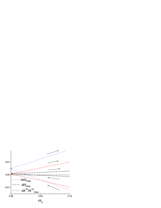
Figure 3: The relative difference in redshift, coordinate time, and beam area, between the propagation in the background of fig. 1 and in a homogeneous background, as a function of the radial coordinate.

We can derive similar expressions for the redshift of a light beam that passes through the center of the inhomogeneity. The geodesic equation (2.6) can be written as

$$\frac{1}{k^{0}}\frac{dk^{0}}{d{\bar{r}}}=-\frac{d\,\ln(1+z)}{d{\bar{r}}}==\pm{\bar{H}}_{i}\frac{\dot{{\bar{R}}}^{\prime}}{1+{\bar{H}}^{2}_{i}{\bar{f}}}\simeq\pm{\bar{H}}_{i}\dot{{\bar{R}}}^{\prime},$$ (4.5)

for incoming and outgoing beams respectively. In this way we find

$$\ln(1+z)= {\bar{H}}_{i}\left(\dot{{\bar{R}}}({\bar{t}}_{s},{\bar{r}}_{s})-\dot{{\bar{R}}}({\bar{t}}_{s},{\bar{r}})\right)$$ (4.6)

$$-{\bar{H}}_{i}^{2}\int_{{\bar{r}}_{s}}^{\bar{r}}\ddot{{\bar{R}}}^{\prime}({\bar{t}}_{s},{\bar{r}})\left({\bar{R}}({\bar{t}}_{s},{\bar{r}}_{s})-{\bar{R}}({\bar{t}}_{s},{\bar{r}})\right)d{\bar{r}}+{\cal O}({\bar{H}}_{i}^{3})$$

for an incoming beam, and

$$\ln(1+z)= {\bar{H}}_{i}\left(\dot{{\bar{R}}}({\bar{t}}_{s},{\bar{r}})-\dot{{\bar{R}}}({\bar{t}}_{s},{\bar{r}}_{s})\right)$$ (4.7)

$$+{\bar{H}}_{i}^{2}\int_{{\bar{r}}_{s}}^{\bar{r}}\ddot{{\bar{R}}}^{\prime}({\bar{t}}_{s},{\bar{r}})\left({\bar{R}}({\bar{t}}_{s},{\bar{r}})-{\bar{R}}({\bar{t}}_{s},{\bar{r}}_{s})\right)d{\bar{r}}+{\cal O}({\bar{H}}_{i}^{3})$$

for an outgoing one. These expressions are confirmed by numerical solutions.

For signals originating at ${\bar{r}}_{s}=1$ and detected at ${\bar{r}}_{o}=0$ the redshifts obey

$$\ln\left(\frac{1+z}{1+z_{FRW}}\right)= {\bar{H}}_{i}^{2}\int_{0}^{1}\ddot{{\bar{R}}}^{\prime}({\bar{t}}_{s},{\bar{r}})\left({\bar{R}}({\bar{t}}_{s},1)-{\bar{R}}({\bar{t}}_{s},{\bar{r}})\right)d{\bar{r}}$$ (4.8)

$$-\frac{{\bar{H}}_{i}^{2}}{2}\ddot{{\bar{R}}}^{\prime}({\bar{t}}_{s},1){\bar{R}}({\bar{t}}_{s},1)+{\cal O}({\bar{H}}_{i}^{3}).$$

For signals originating at ${\bar{r}}_{s}=0$ and detected at ${\bar{r}}_{o}=1$ the r.h.s. of the above equation has the opposite sign. As a result, the redshift difference for signals that cross the inhomogeneity is of ${\cal O}({\bar{H}}^{3}_{i})$. Again, this is in agreement with figs. 2, 3.

5 Luminosity distance and flux conservation

The beam area obeys the second-order differential equation (3.6), whose solution depends crucially on the initial conditions. For initial conditions given by eqs. (3.7), (3.8) and symmetric situations, it is possible to determine the solution analytically. For signals emitted from some point ${\bar{r}}_{s}$ at a time ${\bar{t}}={\bar{t}}_{s}$ and observed at ${\bar{r}}_{o}=0$ we have [33, 16]

$$\sqrt{{\bar{A}}}=(1+z){\bar{R}}({\bar{t}}_{s},{\bar{r}}_{s})\sqrt{{\bar{\Omega}}}.$$ (5.1)

This is in agreement with figs. 2, 3. For signals emitted from the center ${\bar{r}}_{s}=0$ and observed at ${\bar{r}}_{o}$ at a time ${\bar{t}}_{o}$ we have

$$\sqrt{{\bar{A}}}={\bar{R}}({\bar{t}}_{o},{\bar{r}}_{o})\sqrt{{\bar{\Omega}}}.$$ (5.2)

However, for a signal that crosses the inhomogeneity we need to integrate eq. (3.6) from ${\bar{r}}=0$ to ${\bar{r}}_{o}$ with initial conditions determined by the propagation from ${\bar{r}}_{s}$ to ${\bar{r}}=0$. These are different from (3.7), (3.8), so that an analytical solution is not easy.

Figure 4: The deviation of the luminosity distance from its value in a homogeneous background, as a function of the impact parameter.

Using perturbation theory, it is possible to obtain an analytical estimate of the deviation of the luminosity distance from its value in homogeneous cosmology. We consider beam trajectories that start at the boundary of the inhomogeneity, pass through its center and exit from the other side. The optical equation (3.6) can be written in the form

$$\left(\bar{k}^{1}\right)^{2}\frac{d^{2}\sqrt{{\bar{A}}}}{d{\bar{r}}^{2}}+\frac{d\bar{k}^{1}}{d{\bar{\lambda}}}\frac{d\sqrt{{\bar{A}}}}{d{\bar{r}}}=-\frac{3}{2}\bar{\rho}\left(\bar{k}^{0}\right)^{2}\sqrt{{\bar{A}}}.$$ (5.3)

We express $d\bar{k}_{1}/d\bar{\lambda}$ in the above equation using the geodesic equation and obtain

$$\frac{d^{2}\sqrt{\bar{A}}}{d\bar{r}^{2}}+\left(\pm\frac{2\bar{H}_{i}\dot{\bar{R}}^{\prime}}{\sqrt{1+\bar{H}_{i}^{2}{\bar{f}}}}-\frac{\bar{R}^{\prime\prime}}{\bar{R}^{\prime}}+\frac{\bar{H}_{i}^{2}{\bar{f}}^{\prime}}{2(1+\bar{H}_{i}^{2}{\bar{f}})}\right)\frac{d\sqrt{\bar{A}}}{d\bar{r}}=-\frac{3}{2}\bar{\rho}\frac{R^{\prime 2}}{1+\bar{H}_{i}^{2}{\bar{f}}}\sqrt{\bar{A}}$$ (5.4)

where the positive sign in the second term corresponds to ingoing and the negative sign to outgoing geodesics.

We use a simplified initial configuration for this estimate. We take $\bar{\rho}(0,\bar{r})=0$ for $\bar{r}<\bar{r}_{1}$ and $\bar{\rho}(0,\bar{r})=1/(1-\bar{r}_{1}^{3})$ for $\bar{r}>\bar{r}_{1}$. The initial conditions for an ingoing beam can be taken $\sqrt{\bar{A}}({\bar{r}}=1)=0$, $d\sqrt{\bar{A}}({\bar{r}}=1)/d\bar{r}=-1$, without loss of generality. We use the expansion

$$\sqrt{\bar{A}}=\sqrt{\bar{A}^{(0)}}+\bar{H}_{i}\sqrt{\bar{A}^{(1)}}+\bar{H}_{i}^{2}\sqrt{\bar{A}^{(2)}}+{\cal O}({\bar{H}}_{i}^{3}),$$ (5.5)

and calculate $\sqrt{{\bar{A}}^{(i)}}$ in each order of perturbation theory. The calculation in described in the appendix. We point out that our choice of initial configuration, that involves a discontinuous energy density, results in the appearance of $\delta$-function singularities in the second derivatives of ${\bar{R}}$ with respect to ${\bar{r}}$. These must be taken into account in a consistent calculation, as described in the appendix. We have checked that the expressions (5.1) and (5.2) are reproduced correctly by our results, up to second order in ${\bar{H}}_{i}$.

When the photon exits the inhomogeneity at $\bar{r}=1$ we find

$$\sqrt{\bar{A}}(\bar{r}=1) = 2+4\bar{H}_{i}+\left(5-\frac{3}{\bar{r}_{1}^{2}+\bar{r}_{1}+1}\right)\bar{H}_{i}^{2}+{\cal O}({\bar{H}}^{3}_{i})$$ (5.6)

$$\frac{d\sqrt{\bar{A}}}{dr}(\bar{r}=1) = 1+4\bar{H}_{i}+\left(6-\frac{3}{\bar{r}_{1}^{2}+\bar{r}_{1}+1}\right)\bar{H}_{i}^{2}+{\cal O}({\bar{H}}^{3}_{i}).$$ (5.7)

For a homogeneous universe we have

$$\sqrt{\bar{A}}(\bar{r}=1) = 2+4\bar{H}_{i}+2\bar{H}_{i}^{2}$$ (5.8)

$$\frac{d\sqrt{\bar{A}}}{dr}(\bar{r}=1) = 1+4\bar{H}_{i}+3\bar{H}_{i}^{2}.$$ (5.9)

It is clear that the effect of the inhomogeneity is of ${\cal O}({\bar{H}}_{i}^{2})$. This conclusion has been confirmed by numerical solutions of the exact optical equations, without any approximations. Several beam crossings were studied for a multitude of values of ${\bar{H}}_{i}$. The coordinate time ${\bar{t}}_{o}$ needed for the crossing, the redshift $z$ and the beam area ${{\bar{A}}}$ were plotted in terms of ${\bar{H}}_{i}$. The polynomial fits to these plots verify with good precision the conclusions of the present and previous sections: The deviations of ${\bar{t}}_{o}$ and $z$ from their values in a homogeneous background are of ${\cal O}({\bar{H}}_{i}^{3})$, while the deviations of ${\bar{A}}$ are of ${\cal O}({\bar{H}}_{i}^{2})$.

From the above we can conclude that the main effect of an inhomogeneity is to modify the luminosity distance of a light source behind it, while leaving the redshift largely unaffected. In fig. 4 we depict the modification of the luminosity distance $\left(D_{L}-\left(D_{L}\right)_{FRW}\right)/\left(D_{L}\right)_{FRW}$ for light beams that cross a spherical inhomogeneity at various angles. The inhomogeneity is the one employed in the previous section. Its size is approximately $350\,h^{-1}$ Mpc, much larger that what is deduced from observations. We consider realistic inhomogeneities in the following section. The crossing at a varying angle is achieved by choosing different values for the constant $c_{\phi}$ in eq. (2.8). The light source is always located at the same point with ${\bar{r}}_{s}=1.5$. The beam is allowed to propagate until the redshift reaches a certain value $z_{o}\simeq 0.46$. The beam with $c_{\phi}=0$ that goes through the center reaches $r_{o}\simeq 1.5$ at this time. The difference of the resulting luminosity distance from the one in a FRW background is depicted in fig. 4 as a function of ${\tilde{c}}_{\phi}=c_{\phi}/c_{\phi,max}$. The largest value $c_{\phi,max}$ corresponds to beams that are emitted tangentially with respect to the center of symmetry. The angle $\theta$ between the initial direction of the beam and the radial direction is determined through the relation $\sin\theta={\tilde{c}}_{\phi}$. The variable ${\tilde{c}}_{\phi}$ plays the role of an impact parameter, normalized to 1 for light beams emitted tangentially. In fig. 4 we observe that, if ${\tilde{c}}_{\phi}$ is sufficiently small for the light to travel through the central underdense region, the luminosity distance is enhanced relative to the homogeneous case. For larger values of ${\tilde{c}}_{\phi}$ the light travels mainly through the overdense shell and the luminosity distance in reduced.

If the redshift is not affected significantly by the propagation in the inhomogeneous background, the conservation of the total flux implies that the average luminosity distance must be the same as in the homogeneous case [34, 35]. As we have seen, this is not the case for an observer located at the center of an underdensity. The resulting increase in the luminosity distance, arising mainly from the increase in the redshift, can by employed for the explanation of the supernova data, even though the size of the required inhomogeneity is probably in conflict with the observed large-scale structure [15]–[24]. On the other hand, if the source and the observers are located outside the inhomogeneity, as for fig. 4, so that the redshift is essentially unaffected, we expect that the energy flux may be redistributed in various directions but the total flux will be the same as in the homogeneous case [34, 35]. This implies that the integral of $\left(D_{L}-\left(D_{L}\right)_{FRW}\right)/\left(D_{L}\right)_{FRW}$ over all angles must vanish. For an isotropic source the integration over the solid angle is $2\pi\sin\theta\,d\theta$. This is equivalent to the integration over the impact factor ${\tilde{c}}_{\phi}$, with a weight ${\tilde{c}}_{\phi}/\sqrt{1-{\tilde{c}}_{\phi}^{2}}$. The integral of the function depicted in fig. 4 is indeed approximately zero. An analytical proof is very difficult, but a numerical analysis shows that a cancellation at the 90% level takes place between the positive and negative contributions. The remaining deviation from zero is caused by numerical errors and the small (of ${\cal O}({\bar{H}}_{i}^{3})$), but non-vanishing, difference in redshifts in inhomogeneous and homogeneous backgrounds.

6 Multiple crossings

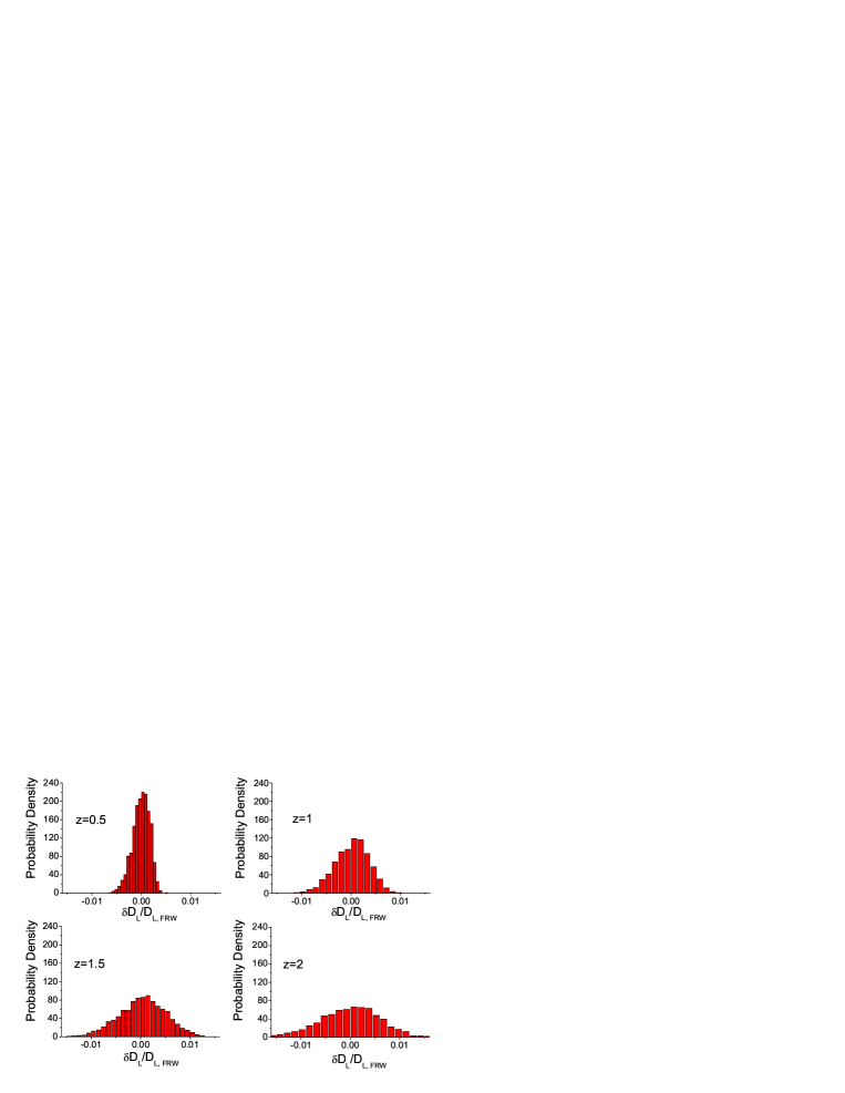
Figure 5: The distribution of luminosity distances for various redshifts in the LTB Swiss-cheese model if the inhomogeneities have a characteristic scale of $40\,h^{-1}$ Mpc.

In this section we consider light beams that pass through several of the inhomogeneities described in the previous sections. The light is emitted at some time ${\bar{t}}_{s}$ from a point with ${\bar{r}}=1$ at the edge of the inhomogeneous region. Its initial direction is assumed to be random. The initial conditions for the beam area are given by eqs. (2.14), (2.15). The light moves through the inhomogeneity and exits from a point with ${\bar{r}}=1$. Subsequently, the beam crosses the following inhomogeneity in a similar fashion. The angle of entry into the new inhomogeneity is assumed to be random again. The initial conditions are set by the values of $\sqrt{{\bar{A}}}$ and $d\sqrt{{\bar{A}}}/{d{\bar{\lambda}}}$ at the end of the first crossing. This process is repeated until the light arrives at the observer. Of course, as time passes the profile of the inhomogeneities changes, as depicted in fig. 1.

The assumption of entry into a spherical inhomogeneity at a random azimuthal angle is realized by selecting the impact factor ${\tilde{c}}_{\phi}$ with a probability $\sim{\tilde{c}}_{\phi}d{\tilde{c}}_{\phi}$. The absence of the denominator $\sqrt{1-{\tilde{c}}_{\phi}^{2}}$ that appears in the weight employed in the previous section is justified by the fact that the source is located far from the center of the inhomogeneity, so that ${\tilde{c}}_{\phi}\ll 1$. This is not strictly true for the first 1 or 2 crossings, but the induced error is small. In order to place the observer outside the inhomogeneities we always replace the final spherical region crossed by the beam with a homogeneous configuration.

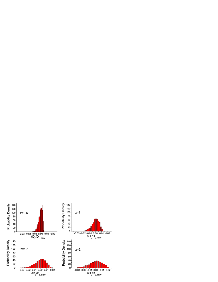
Figure 6: Same as in fig. 5 for a characteristic scale of $133\,h^{-1}$ Mpc.

The essence of our procedure is that the light beam encounters various inhomogeneities at various angles along its path. In this section we consider the propagation of the beam only in the intervals $0\leq\tilde{r}\leq 1$ of coordinate systems with origins at the center of the various inhomogeneities. This means that we neglect the homogeneous region between the inhomogeneities that we assumed in the previous region. (Essentially we assume that its width is negligible.) The reason for this omission is that the presence of the homogeneous region generates a bias towards negligible deviations of the luminosity distance from its value in a homogeneous cosmology. For example, if we consider light propagation in the intervals $0\leq\tilde{r}\leq 1.5$ as in the previous section, a large number of beam trajectories propagate only within the homogeneous regions with $1\leq\tilde{r}\leq 1.5$. These give a luminosity distance for the source equal to that in the FRW cosmology. On the other hand, there are trajectories that propagate through the inhomogeneities, for which the cancellation between positive and negative contributions results in a negligible total deviation of the luminosity distance from the value in a homogeneous background. It is the latter events that we are interested in, while the former are rather unphysical.

The procedure we outlined above has an unsatisfactory element. The spherical inhomogeneities are assumed to follow each other continuously along the beam trajectory. If the angles of entry of the beam are non-zero, the resulting geometry implies that there is an overlap of the inhomogeneities outside the beam trajectory. This problem cannot be corrected as long as the assumption of spherical symmetry of the inhomogeneities is maintained. A choice must be made between an artificial bias in the luminosity distance if intermediate homogeneous regions are introduced, or the overlap of the inhomogeneities outside the beam trajectory. We have chosen the second option, as we believe that it provides a more reliable estimate of the distribution of luminosity distances.

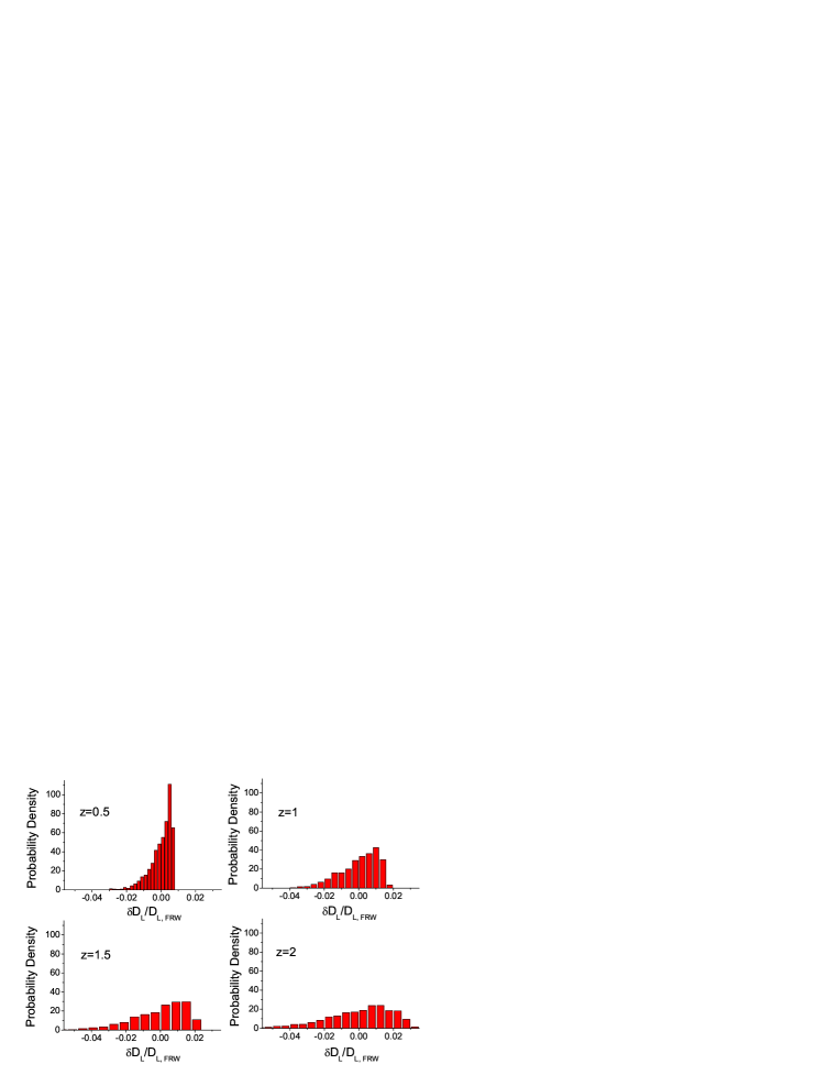
Figure 7: Same as in fig. 5 for a characteristic scale of $400\,h^{-1}$ Mpc.

The total number of crossings determines the redshift and the final beam area, related to the luminosity distance. We determine the arrival time at the observer by requiring that the redshift reach a specific value. We repeat the calculation many times (at least 1000) for each value of the redshift and plot the resulting distribution of luminosity distances. The emission time is such that the arrival time is ${\bar{t}}_{o}\simeq 284$ for all the redshifts that we consider. At this time the profile of the inhomogeneity is very similar to the curve in fig. 1 with the largest deviation from 1. The deviations of the exact arrival time ${\bar{t}}_{o}$ from the time in a homogeneous background is one order of magnitude smaller than the respective deviation for the luminosity distance. This is in agreement with the discussion in the previous section.

In figs. 5, 6, 7 we depict the distributions of the deviations of the luminosity distances from the value in a homogeneous background for various redshifts. The three figures correspond to inhomogeneities with different characteristic length scales at the time of the emission of light. The background through which the light propagates is constructed as described in the previous sections. At the initial time ${\bar{t}}_{i}=0$ the inhomogeneities have the profile descibed in the previous section with $\epsilon_{1}=-0.01$. The subsequent evolution is depicted in fig. 1. The characteristic length scale of the inhomogeneities relative to the distance to the horizon at the time ${\bar{t}}_{i}=0$ is $r_{0}/(H^{-1}_{i})={\bar{H}}_{i}$. This quantity does not appear in the rescaled evolution equations for the background. It appears only in the rescaled geodesic equations. For this reason we can use the same background, with an evolution depicted in fig. 1, in order to discuss inhomogeneities of various length scales. The important phenomenological quantity is the scale of the inhomogeneities today. This is given by $R(t_{f},r_{0})/(H^{-1}_{f})=\dot{R}(t_{f},r_{0})=\dot{{\bar{R}}}({\bar{t}}_{f},1){\bar{H}}_{i}$. The rescaled present time ${\bar{t}}_{f}$ is equal to the time of arrival of light signals to the observer ${\bar{t}}_{o}$ for all the cases we consider. As we mentioned already, ${\bar{t}}_{f}={\bar{t}}_{o}\simeq 284$. Our solution has $\dot{{\bar{R}}}({\bar{t}}_{o})=0.133$. Using $H^{-1}_{f}=3\times 10^{3}\,h^{-1}$ Mpc we have $R(t_{f},r_{0})=400\,h^{-1}{\bar{H}}_{i}$ Mpc.

The three figures 5, 6, 7 correspond to ${\bar{H}}_{i}=1/10$, 1/3, 1, respectively. They describe the effect on the propagation of light of inhomogeneities with sizes 40, 133, $400\,h^{-1}$ Mpc today. The present profile of the inhomogeneities has a density contrast ${\cal O}(1)$. Their evolution, as modelled by the LTB metric, is roughly consistent with the standard theory of structure growth. The choices ${\bar{H}}_{i}=1/3$ and 1 lead to present-day inhomogeneities with length scales larger than those in typical observations. The size of the same perturbations at horizon crossing is larger than the value $\sim 10^{-5}$ implied by the CMB. However, we have included them for two reasons. Firstly, because there are indications that the presence of such large structures may be supported by observations [25, 26]. Secondly, because we would like to understand if inhomogeneities with sizes comparable to the horizon distance can have a significant effect on the luminosity distance for a random location of the observer.

The total integral of the distributions has been normalized to 1 in all cases, so that they are in fact probability densities. They have similar profiles that are asymmetric around zero. Each distribution has a maximum at a value larger than zero and a long tail towards negative values. The average deviation is zero to a good approximation in all cases. This is expected according to our discussion of flux conservation in the previous section. As long as the light propagation in an inhomogeneous background does not modify significantly the redshift, the energy may be redistributed in various directions, but the total flux is conserved and remains the same as in a FRW background.

The longer tail of the distribution towards luminosity distances smaller than the one in a homogeneous background is a consequence of the presence of a thin and dense spherical shell around each central underdensity. The number of beam trajectories that propagate through several shells is small. However, the focusing of the beam is substantial for such beams and the resulting luminosity distance much shorter than the average. The effect of the long tail is compensated by the shift of the maximum of the distribution towards positive values. The form of the distribution is very similar to that derived in studies modelling the inhomogeneities through the standard Swiss-cheese model [11]. In that case the strong focusing is generated by the very dense concentration of matter at the center of each spherical inhomogeneity. We emphasize, however, that the two models have a different region of applicability. The standard Swiss-cheese model is appropriate for length scales of ${\cal O}(1)\,h^{-1}$ Mpc or smaller, while the LTB Swiss-cheese model for scales of ${\cal O}(10)\,h^{-1}$ Mpc or larger.

7 Determination of cosmological parameters

Figure 8: The relative deviation of the luminosity distance from its value for $w=0$ (non-relativistic matter) in homogeneous cosmology.

The form of the distributions can be quantified in terms of two parameters: The width of the distribution $\delta_{d}$ and the location of its maximum $\delta_{m}>0$. The first one characterizes the error induced to cosmological parameters derived through the curve of the luminosity distance as a function of redshift, while the second one the bias in such determinations. As discussed extensively in ref. [11], a small sample of data is expected to favour values of the luminosity distance near the maximum of the distribution, and thus generate a bias. In figs. 5, 6, 7 we observe that both $\delta_{d}$ and $\delta_{m}$ grow with inreasing redshift $z$ and scale ${\bar{H}}_{i}$. For ${\bar{H}}_{i}=1/10$ the average width $\delta_{d}$ increases from approximately 0.005 to 0.01 as $z$ increases from 0.5 to 2. The maximum is $\delta_{m}\mathrel{\vbox{\hbox{$<$}\nointerlineskip\hbox{$\sim$}}}0.002$ for all $z$. The asymmetry of the distribution is very small. For ${\bar{H}}_{i}=1/3$ the average width increases from approximately 0.005 to 0.02 as $z$ increases from 0.5 to 2. The maximum is $\delta_{m}\mathrel{\vbox{\hbox{$<$}\nointerlineskip\hbox{$\sim$}}}0.002$ for all $z$. The asymmetry of the distribution and the longer tail towards negative values are clearly visible in fig. 6. For ${\bar{H}}_{i}=1$ the average width increases from approximately 0.01 to 0.04 as $z$ increases from 0.5 to 2. The maximum increases from 0.005 to 0.01. The asymmetry of the distribution is very distinctive in fig. 7.

The values of $\delta_{d}$ and $\delta_{m}$ are very small for all the values of ${\bar{H}}_{i}$ that we considered. This implies that we do not expect a significant effect on the cosmological parameters. As an interesting example we consider the parameter $w$ that appears in the equation of state of the cosmological fluid. In homogeneous cosmology the luminosity distance is a function of $w$ and the redshift $z$. The relative deviation of the luminosity distance from its value for $w=0$ (non-relativistic matter) is

$$s(w,z)=\frac{D_{L}(w,z)}{D_{L}(0,z)}-1=\frac{1}{1+3w}\frac{1-\left(z+1\right)^{-(1+3w)/2}}{1-\left(z+1\right)^{-1/2}}-1.$$ (7.1)

We depict this function in fig. 8. For $w=-1$ the luminosity distance is larger by roughly 35% relative to $w=0$ for $z=0.5$. For $z=1$ the relative increase is approximately 70%.

The deviations of $\delta_{d}(z)$ and $\delta_{m}(z)$ from zero because of the presence of inhomogeneities can be attributed to deviations of $w$ from zero if the cosmology is assumed to be homogeneous. This can be achieved by identifying $\delta_{d}(z)$ or $\delta_{m}(z)$ with $s(w,z)$. For small $w$ we have

$$s(w,z)\simeq-3\left(1-\frac{1}{2}\frac{\ln(z+1)}{(z+1)^{1/2}-1}\right)w=-\alpha(z)w.$$ (7.2)

We depict the function $\alpha(z)$ in fig. 9. For a given value of $z$ we can derive effective values of $w$ from the relations $w_{eff}=-\delta_{d,m}(z)/\alpha(z)$. It is clear from the values we quoted above for $\delta_{d}$, $\delta_{m}$ and fig. 9 that $|w_{eff}|\ll 1$. As a result, for a random location of the observer the perceived acceleration of the Universe cannot be attributed to the modification of the luminosity distance by large-scale inhomogeneities, even when their characteristic scale is smaller than the horizon distance by less than a factor of 10.

Figure 9: The function $\alpha(z)=-\left.\partial s(w,z)/\partial w\right|_{w=0}$.

On the other hand, the presence of inhomogeneities induces a statistical error in the value of $w$ deduced from astrophysical data, as well as a shift of its average value if the sample is small. According to our results, for ${\bar{H}}_{i}=1/10$ (and present size of the inhomogeneities $40\,h^{-1}$ Mpc) the error is $\delta w\simeq 0.015$ for all $z$ between 0.5 and 2, while the average value $\bar{w}$ for a small sample is negative and of ${\cal O}(10^{-3})$. For ${\bar{H}}_{i}=1/3$ (and present size of the inhomogeneities $133\,h^{-1}$ Mpc) the error increases from 0.015 to 0.025 as $z$ increases from 0.5 to 2, while the average value $\bar{w}$ is again negative and of ${\cal O}(10^{-3})$. For ${\bar{H}}_{i}=1$ (and present size of the inhomogeneities $400\,h^{-1}$ Mpc) the error increases from 0.03 to 0.05, while the average is ${\bar{w}}\simeq-0.015$. The shift in the average value is always smaller than a standard deviation.

The values of $\delta_{d}$ and $\delta_{m}$ can be compared to those generated by the effects of gravitational lensing at scales typical of galaxies or clusters of galaxies. At such scales the Universe is modelled through the standard Swiss-cheese model, with the mass of each inhomogeneity concentrated in a very dense object at its center [11]. The typical values of $\delta_{d}$ and $\delta_{m}$ are larger by at least an order of magnitude than the ones we obtained. The reason is that in our model the density contrast is always of ${\cal O}(1)$. Our study indicates that the effect on the luminosity distance grows when the length scale of the inhomogeneities increases and becomes comparable to the horizon distance. However, the strong lensing effect of a high concentration of mass, such as a galaxy or cluster of galaxies, gives a much larger effect.

We conclude that within our model the presence of inhomogeneities with large length scales, even comparable to the horizon distance, and density contrast of ${\cal O}(1)$ does not influence significantly the propagation of light if the source and the observer have random locations. It is possible that our modelling of the Universe is lacking some essential feature that could generate a significant effect on the luminosity distance. For example, it has been suggested that large fluctuations in the spatial curvature may result in a strong backreaction on the overall expansion [37]. Unfortunately, there are no known exact models that realize such a scenario. In their absence the effect on the luminosity distance cannot be computed. In our model, there are variations of the local curvature which result in the collapse of the overdense regions (either central overdensities, or shells surrounding underdensities). The evolution is in approximate agreement with the standard theory of structure formation. It seems difficult to reconcile a much larger local curvature with a large-scale structure consistent with observations. Another possibility is that the assumed spherical symmetry of the inhomogeneities in our modelling of the Universe is too constraining. It is possible that photon propagation through inhomogeneities without such a symmetry results in a stronger modification of the luminosity distance. This point will be the subject of a future investigation.

Acknowledgments
This work was supported by the research program “Pythagoras II” (grant 70-03-7992) of the Greek Ministry of National Education, partially funded by the European Union.

8 Appendix

In this appendix we describe the solution of eq. (5.4) through the use of perturbation theory in ${\bar{H}}_{i}$. In this way we demonstrate that a spherical inhomogeneity induces a deviation of the luminosity distance from its value in a homogeneous background which is of ${\cal O}({\bar{H}}_{i}^{2})$.

The null constraint (2.7), keeping terms up to ${\cal O}(\bar{H}_{i})$, is ${d\bar{t}}/{d\bar{r}}=\pm\bar{H}_{i},$ with the negative sign corresponding to ingoing and the positive to outgoing geodesics. We can set $t_{s}=0$ so the geodesic inside the inhomogeneity is

$$\bar{t}=-\bar{H}_{i}(\bar{r}-\bar{r}_{0})+{\cal O}(\bar{H}_{i}^{2})$$ (8.3)

for ingoing, and

$$\bar{t}=\bar{H}_{i}(\bar{r}+\bar{r}_{0})+{\cal O}(\bar{H}_{i}^{2})$$ (8.4)

for outgoing geodesics. We can treat $\bar{t}$ as an ${\cal O}(\bar{H}_{i})$ quantity.

The initial configuration we use for this estimate has $\bar{\rho}(0,\bar{r})=0$ for $\bar{r}<\bar{r}_{1}$ and $\bar{\rho}(0,\bar{r})=1/(1-\bar{r}_{1}^{3})$ for $\bar{r}>\bar{r}_{1}$. From (3.5) we can calculate various derivatives of $\bar{R}$ at $\bar{t}=0$:

$$\dot{\bar{R}}^{\prime}(\bar{t},\bar{r})=\dot{\bar{R}}^{\prime}(0,\bar{r})+\bar{t}\ddot{\bar{R}}^{\prime}(0,\bar{r})+{\cal O}(\bar{H}_{i}^{2}),$$ (8.5)

$$\frac{\bar{R}^{\prime\prime}}{\bar{R}^{\prime}}(\bar{t},\bar{r})=\frac{\bar{t}^{2}}{2}\ddot{\bar{R}}^{\prime\prime}(0,\bar{r})+{\cal O}(\bar{H}_{i}^{3}).$$ (8.6)

For $\bar{r}>\bar{r}_{1}$ we have

$$\ddot{\bar{R}}^{\prime}(0,\bar{r}) = \frac{r^{3}+2\bar{r}_{1}^{3}}{2r^{3}\left(\bar{r}_{1}^{3}-1\right)}$$ (8.7)

$$\ddot{\bar{R}}^{\prime\prime}(0,\bar{r}) = -\frac{3\bar{r}_{1}^{3}}{r^{4}\left(\bar{r}_{1}^{3}-1\right)}.$$ (8.8)

For $\bar{r}<\bar{r}_{1}$ both $\ddot{\bar{R}}^{\prime}(0,\bar{r})$ and $\ddot{\bar{R}}^{\prime\prime}(0,\bar{r})$ are zero. For the initial configuration that we assume, $\ddot{\bar{R}}$ is a continuous function of ${\bar{r}}$. However, $\ddot{\bar{R}}^{\prime}$ is discontinuous at ${\bar{r}}={\bar{r}}_{1}$ and ${\bar{r}}=1$, while $\ddot{\bar{R}}^{\prime\prime}$ has $\delta$-function singularities at the same points.

The initial conditions for the solution of eq. (5.4) for an ingoing beam can be taken $\sqrt{\bar{A}}(1)=0$, $d\sqrt{\bar{A}}(1)/d\bar{r}=-1$, without loss of generality. We use the expansion

$$\sqrt{\bar{A}}=\sqrt{\bar{A}^{(0)}}+\bar{H}_{i}\sqrt{\bar{A}^{(1)}}+\bar{H}_{i}^{2}\sqrt{\bar{A}^{(2)}}+{\cal O}({\bar{H}}_{i}^{3}).$$ (8.9)

To zeroth order in $\bar{H}_{i}$, eq. (5.4) becomes ${d^{2}\sqrt{\bar{A}^{(0)}}}/{d\bar{r}^{2}}=0$, with solution $\sqrt{\bar{A}^{(0)}}(\bar{r})=-(r-1)$ for ingoing and $\sqrt{\bar{A}^{(0)}}(\bar{r})=r+1$ for outgoing beams. To first order in $\bar{H}_{i}$, eq. (5.4) gives ${d\sqrt{\bar{A}^{(1)}}}/{d\bar{r}}=-2$, with solution $\sqrt{\bar{A}^{(1)}}(\bar{r})=r^{2}-2r+1$ for ingoing and $\sqrt{\bar{A}^{(1)}}(\bar{r})=r^{2}+2r+1$ for outgoing beams.

To second order in $\bar{H}_{i}$, and for $\bar{r}>\bar{r}_{1}$ and ingoing geodesics, we obtain

$$\frac{d^{2}\sqrt{\bar{A}^{(2)}}}{d\bar{r}^{2}}+\Biggl{(}2\bar{t}(\bar{r})\ddot{\bar{R}}^{\prime}(0,\bar{r})-\frac{\bar{t}^{2}}{2}\ddot{\bar{R}}^{\prime\prime}(0,\bar{r}) + \frac{{\bar{f}}^{\prime}(\bar{r})}{2}\Biggr{)}\frac{d\sqrt{\bar{A}^{(0)}}}{d\bar{r}}+2\frac{d\sqrt{\bar{A}^{(1)}}}{d\bar{r}}$$ (8.10)

$$= -\frac{3}{2}\bar{\rho}(0,\bar{r})\sqrt{\bar{A}^{(0)}}.$$

For $\bar{r}<\bar{r}_{1}$ and ingoing geodesics, we have

$$\frac{d^{2}\sqrt{\bar{A}^{(2)}}}{d\bar{r}^{2}}+\frac{{\bar{f}}^{\prime}(\bar{r})}{2}\frac{d\sqrt{\bar{A}^{(0)}}}{d\bar{r}}+2\frac{d\sqrt{\bar{A}^{(1)}}}{d\bar{r}}=0.$$ (8.11)

For $\bar{r}<\bar{r}_{1}$ and outgoing geodesics, we have

$$\frac{d^{2}\sqrt{\bar{A}^{(2)}}}{d\bar{r}^{2}}+\frac{{\bar{f}}^{\prime}(\bar{r})}{2}\frac{d\sqrt{\bar{A}^{(0)}}}{d\bar{r}}-2\frac{d\sqrt{\bar{A}^{(1)}}}{d\bar{r}}=0.$$ (8.12)

Finally, for $\bar{r}>\bar{r}_{1}$ and outgoing geodesics, we obtain

$$\frac{d^{2}\sqrt{\bar{A}^{(2)}}}{d\bar{r}^{2}}+\Biggl{(}-2\bar{t}(\bar{r})\ddot{\bar{R}}^{\prime}(0,\bar{r})-\frac{\bar{t}^{2}}{2}\ddot{\bar{R}}^{\prime\prime}(0,\bar{r}) + \frac{{\bar{f}}^{\prime}(\bar{r})}{2}\Biggr{)}\frac{d\sqrt{\bar{A}^{(0)}}}{d\bar{r}}-2\frac{d\sqrt{\bar{A}^{(1)}}}{d\bar{r}}$$ (8.13)

$$= -\frac{3}{2}\bar{\rho}(0,\bar{r})\sqrt{\bar{A}^{(0)}}.$$

The above equations can be solved analytically through simple integration, with the values at the end of each interval determining the initial conditions for the next one. The only non-trivial point is that the $\delta$-function singularities of $\ddot{\bar{R}}^{\prime\prime}$ at ${\bar{r}}={\bar{r}}_{1}$ and ${\bar{r}}=1$ induce discontinuities in the values of ${d\sqrt{\bar{A}^{(2)}}}/{d\bar{r}}$ at these points. These must be taken into account in a consistent calculation. The discontinuities can be easily determined through the integration of eqs. (8.10)–(8.13) in an infinitesimal interval around each of these points. The remaining calculation is straightforward. When the photon exits the inhomogeneity at $\bar{r}=1$ we find that $\sqrt{{\bar{A}}}$ is given by eq. (5.6).

References

References

-
[1]
A. G. Riess et al. [Supernova Search Team Collaboration],
Astron. J. 116 (1998) 1009
[arXiv:astro-ph/9805201];
Astrophys. J. 607 (2004) 665
[arXiv:astro-ph/0402512];
S. Perlmutter et al. [Supernova Cosmology Project Collaboration], Astrophys. J. 517 (1999) 565 [arXiv:astro-ph/9812133]. -
[2]
W. J. Percival et al. [The 2dFGRS Collaboration],
Mon. Not. Roy. Astron. Soc. 327 (2001) 1297
[arXiv:astro-ph/0105252];
J. L. Sievers et al., Astrophys. J. 591 (2003) 599 [arXiv:astro-ph/0205387]. - [3] D. N. Spergel et al. [WMAP Collaboration], Astrophys. J. Suppl. 148 (2003) 175 [arXiv:astro-ph/0302209].
-
[4]
S. Rasanen,
JCAP 0402 (2004) 003
[arXiv:astro-ph/0311257];
E. W. Kolb, S. Matarrese, A. Notari and A. Riotto, Phys. Rev. D 71 (2005) 023524 [arXiv:hep-ph/0409038]. -
[5]
T. Futamase and M. Sasaki,
Phys. Rev. D 40 (1989) 2502.
M. Kasai, T. Futamase and F. Takahara, Phys. Lett. A 147 (1990) 97.
F. Hadrovic and J. Binney, arXiv:astro-ph/9708110.
T. Pyne and M. Birkinshaw, Mon. Not. Roy. Astron. Soc. 348 (2004) 581 [arXiv:astro-ph/0310841]. -
[6]
E. W. Kolb, S. Matarrese, A. Notari and A. Riotto,
Phys. Rev. D 71 (2005) 023524
[arXiv:hep-ph/0409038].
E. Barausse, S. Matarrese and A. Riotto, Phys. Rev. D 71 (2005) 063537 [arXiv:astro-ph/0501152]. - [7] R. K. Sachs, Proc. Roy. Soc. London A 264 (1961) 309.
- [8] R. Kantowski, Astrophys. J. 155 (1969) 89.
- [9] A. Einstein and E. G. Straus, Rev. Mod. Phys. 17 (1945) 120; ibid. 18 (1946) 148.
-
[10]
R. Kantowski,
Astrophys. J. 507 (1998) 483
[arXiv:astro-ph/9802208];
Phys. Rev. D 68 (2003) 123516
[arXiv:astro-ph/0308419];
R. Kantowski and R. C. Thomas, Astrophys. J. 561 (2001) 491 [arXiv:astro-ph/0011176]. -
[11]
D. E. Holz and R. M. Wald,
Phys. Rev. D 58 (1998) 063501
[arXiv:astro-ph/9708036];
D. E. Holz, Astrophys. J. 506, L1 (1998) [arXiv:astro-ph/9806124];
D. E. Holz and E. V. Linder, Astrophys. J. 631, 678 (2005) [arXiv:astro-ph/0412173]. -
[12]
M. Sereno, G. Covone, E. Piedipalumbo and R. de Ritis,
Mon. Not. Roy. Astron. Soc. 327 (2001) 517
[arXiv:astro-ph/0102486];
M. Sereno, E. Piedipalumbo and M. V. Sazhin, Mon. Not. Roy. Astron. Soc. 335 (2002) 1061 [arXiv:astro-ph/0209181]. - [13] C. C. Dyer and R. C. Roeder, Astrophys. J. 180 (1973) L31; ibid. 189 (1974) 167
-
[14]
G. Lemaitre,
Gen. Rel. Grav. 29 (1997) 641;
R. C. Tolman, Proc. Nat. Acad. Sci. 20 (1934) 169;
H. Bondi, Mon. Not. Roy. Astron. Soc. 107 (1947) 410. - [15] N. Mustapha, C. Hellaby and G. F. R. Ellis, Mon. Not. Roy. Astron. Soc. 292 (1997) 817 [arXiv:gr-qc/9808079].
- [16] M. N. Celerier, Astron. Astrophys. 353 (2000) 63 [arXiv:astro-ph/9907206].
-
[17]
H. Iguchi, T. Nakamura and K. i. Nakao,
Prog. Theor. Phys. 108 (2002) 809
[arXiv:astro-ph/0112419];
K. Bolejko, arXiv:astro-ph/0512103;
R. Mansouri, arXiv:astro-ph/0512605;
R. A. Vanderveld, E. E. Flanagan and I. Wasserman, Phys. Rev. D 74 (2006) 023506 [arXiv:astro-ph/0602476];
D. Garfinkle, Class. Quant. Grav. 23 (2006) 4811 [arXiv:gr-qc/0605088];
D. J. H. Chung and A. E. Romano, Phys. Rev. D 74 (2006) 103507 [arXiv:astro-ph/0608403]. - [18] S. Rasanen, JCAP 0411 (2004) 010 [arXiv:gr-qc/0408097]; JCAP 0611 (2006) 003 [arXiv:astro-ph/0607626].
- [19] J. W. Moffat, JCAP 0510 (2005) 012 [arXiv:astro-ph/0502110]; arXiv:astro-ph/0505326.
-
[20]
H. Alnes, M. Amarzguioui and O. Gron,
JCAP 0701 (2007) 007
[arXiv:astro-ph/0506449];
Phys. Rev. D 73 (2006) 083519
[arXiv:astro-ph/0512006];
H. Alnes and M. Amarzguioui, Phys. Rev. D 75 (2007) 023506 [arXiv:astro-ph/0610331]. - [21] K. Enqvist and T. Mattsson, JCAP 0702 (2007) 019 [arXiv:astro-ph/0609120].
- [22] C. H. Chuang, J. A. Gu and W. Y. Hwang, arXiv:astro-ph/0512651.
- [23] P. S. Apostolopoulos, N. Brouzakis, N. Tetradis and E. Tzavara, JCAP 0606 (2006) 009 [arXiv:astro-ph/0603234].
- [24] T. Biswas, R. Mansouri and A. Notari, arXiv:astro-ph/0606703.
- [25] K. Tomita, Astrophys. J. 529, 26 (2000); Astrophys. J. 529, 38 (2000); Mon. Not. Roy. Astron. Soc. 326 (2001) 287 [arXiv:astro-ph/0011484].
- [26] W. J. Frith, G. S. Busswell, R. Fong, N. Metcalfe and T. Shanks, Mon. Not. Roy. Astron. Soc. 345 (2003) 1049 [arXiv:astro-ph/0302331].
- [27] N. Brouzakis, N. Tetradis and E. Tzavara, JCAP 0702 (2007) 013 [arXiv:astro-ph/0612179].
- [28] P. Schneider, J. Ehlers and E. E. Falco, Gravitational Lenses, Springer-Verlag, Berlin.
- [29] T. Biswas and A. Notari, arXiv:astro-ph/0702555.
- [30] W. Israel, Nuovo Cim. B 44 (1966) 1.
-
[31]
H. Sato,
Prog. Theor. Phys. 76 (1986) 1250;
V. A. Berezin, V. A. Kuzmin and I. I. Tkachev, Phys. Rev. D 36 (1987) 2919;
S. Khakshournia and R. Mansouri, Phys. Rev. D 65 (2002) 027302 [arXiv:gr-qc/0307023]. -
[32]
J. E. Gunn and J. R. I. Gott,
Astrophys. J. 176, 1 (1972);
A. Cooray and R. Sheth, Phys. Rept. 372 (2002) 1 [arXiv:astro-ph/0206508]. -
[33]
M. H. Partovi and B. Mashhoon,
Astrophys. J. 276 (1984) 4.
N. P. Humphreys, R. Maartens and D. R. Matravers, Astrophys. J. 477 (1997) 47 [arXiv:astro-ph/9602033]. - [34] S. Weinberg, Astrophys. J. 208 (1976) L1
- [35] H. G. Rose, Astrophys. J. 560 (2001) L15 [arXiv:astro-ph/0106489].
- [36] G. Aldering, A. G. Kim, M. Kowalski, E. V. Linder and S. Perlmutter, Astropart. Phys. 27 (2007) 213 [arXiv:astro-ph/0607030].
-
[37]
T. Buchert,
Class. Quant. Grav. 23 (2006) 817
[arXiv:gr-qc/0509124];
T. Buchert, J. Larena and J. M. Alimi, Class. Quant. Grav. 23 (2006) 6379 [arXiv:gr-qc/0606020].