Direct evidence of acceleration from distance modulus redshift graph

Abstract

The energy conditions give upper bounds on the luminosity distance. We apply these upper bounds to the 192 essence supernova Ia data to show that the Universe had experienced accelerated expansion. This conclusion is drawn directly from the distance modulus-reshift graph. In addition to be a very simple method, this method is also totally independent of any cosmological model. From the degeneracy of the distance modulus at low redshift, we argue that the choice of $w_{0}$ for probing the property of dark energy is misleading. One explicit example is used to support this argument.

I Introduction

Ever since the discovery of the accelerated expansion of the Universe by the supernova (SN) Ia observations agr98 , many efforts have been made to understand the mechanism of this accelerated expansion. Although different observations pointed to the existence of dark energy which has negative pressure and contributes about 72% of the matter content of the Universe riess ; astier ; riess06 ; wmap3 ; sdss , the nature of dark energy is still a mystery to us. For a review of dark energy models, one may refer to Ref. DE .

Due to the lack of a satisfactory dark energy model, many parametric and non-parametric model-independent methods were proposed to study the property of dark energy and the geometry of the Universe virey ; sturner ; gong06 ; gong07 ; astier01 ; huterer ; weller ; alam ; gong04 ; gong05 ; lind ; jbp ; par1 ; par2 ; par3 ; par4 ; par5 ; gong04a ; wang05 ; jbp05 ; nesseris6a ; berger ; sahni06 ; lihong ; yun06 ; evldh ; saini ; jbp06 ; nesseris05 . In the reconstruction of the deceleration parameter $q(z)$, it was found that the strongest evidence of acceleration happens at redshift $z\sim 0.2$ virey ; sturner ; gong06 ; gong07 . The sweet spot of the equation of state parameter $w(z)$ was found to be around the redshift $z\sim 0.2-0.5$ gong07 ; astier01 ; huterer ; weller ; alam ; gong04 ; gong05 .

The energy conditions were also used to study the expansion of the Universe in visser ; alcaniz ; aasen . The energy condition $\rho+3p\geq 0$ is equivalent to $q(z)\geq 0$, and the energy condition $\rho+p\geq 0$ is equivalent to $\dot{H}\leq 0$ for a flat universe. These conditions give lower bounds on the Hubble parameter $H(z)$, and therefore upper bounds on the luminosity distance. These bounds can be put in the distance modulus-redshift graph to give direct model independent evidence of accelerated expansion. On the other hand, to the lowest order, the luminosity distance $d_{L}(z)$ is independent of any cosmological model. In the low $z$ region ($z\leq 0.1$), $d_{L}(z)$ is degenerate. So different dark energy models will give almost the same $d_{L}(z)$ in the low $z$ region and the current value $w_{0}$ of $w(z)$ is not well constrained. That is the main reason why the sweet spot is found to be around $z\sim 0.3$. In this paper, we compare two dark energy models which differ only in the low $z$ region to further explain the consequence of the degeneracy.

This paper is organized as follows. In section II, we apply the energy conditions to the flat universe to show model independent evidence of accelerated expansion. In section III, we use two dark energy models to argue as to why the value of $w_{0}$ is not good for exploring the property of dark energy. The energy conditions are applied to the non-flat universe in section IV. In section V, we conclude the paper with some discussions.

II Distance modulus redshift graph

The strong energy condition $\rho+3p\geq 0$ and $\rho+p\geq 0$ tells us that

$$q(t)=-\ddot{a}/(aH^{2})\geq 0,\quad\dot{H}-\frac{k}{a^{2}}\leq 0$$ (1)

The Hubble parameter $H(t)=\dot{a}/a$ and the deceleration parameter $q(t)$ are related by the following equation,

$$H(z)=H_{0}\exp\left[\int^{z}_{0}[1+q(u)]d\ln(1+u)\right],$$ (2)

where the subscript 0 means the current value of the variable. Therefore, the strong energy condition requires that

$$H(z)\geq H_{0}(1+z),$$ (3)

and

$$\quad H(z)\geq H_{0}\sqrt{1-\Omega_{k}+\Omega_{k}(1+z)^{2}},$$ (4)

for redshift $z=a_{0}/a-1\geq 0$. Note that the satisfying of Eq. (3) guarantees the satisfying of Eq. (4). Although Eq. (3) is derived from Eq. (1), they are not equivalent. Due to the integration effect, we cannot derive Eq. (1) from Eq. (3). If the strong energy condition is always satisfied, i.e., the Universe always experiences decelerated expansion, then there is a lower bound on the Hubble parameter given by Eq. (3). When Eq. (3) is violated, we conclude that the Universe once experienced accelerated expansion. On the other hand, if the Universe always experiences accelerated expansion, then there is an upper bound on the Hubble parameter. So if the Hubble parameter satisfies Eq. (3), then we conclude that the Universe once experienced decelerated expansion. The satisfying of Eq. (4) means that the Universe has experienced non-super-acceleration for a flat universe. From the above discussion, it is clear that these energy conditions can be used to show the evidence of acceleration and super-acceleration in the luminosity distance redshift diagram. We consider a flat universe first. The luminosity distance is

$$d_{L}(z)=(1+z)\int_{0}^{z}\frac{dz^{\prime}}{H(z^{\prime})}.$$ (5)

The extinction-corrected distance modulus $\mu(z)=5\log_{10}[d_{L}(z)/{\rm Mpc}]+25$. Substitute Eqs. (3) and (4) into Eq. (5), we get the upper bounds on the luminosity distance

$$H_{0}d_{L}(z)\leq z(1+z),\quad H_{0}d_{L}(z)\leq(1+z)\ln(1+z).$$ (6)

Again, Eq. (6) is derived from Eq. (1), but Eqs. (1) and (6) are not equivalent because the luminosity distance involves integration. To understand the integration effect, we use the $\Lambda$CDM model as an example. For $\Lambda$CDM model, the Universe experienced accelerated expansion in the redshift region $z\lesssim 0.76$ and decelerated expansion in the redshift region $z\gtrsim 0.76$. In other words, the strong energy condition is violated in the redshift region $z\lesssim 0.76$, and satisfied in the redshift region $z\gtrsim 0.76$. We plot the distance modulus $\mu(z)$ for the $\Lambda$CDM model in Fig. 1. From Fig. 1, we see that $\mu(z)$ for the $\Lambda$CDM model is outside the bound given by the lower solid line up to the redshift $z\sim 7$. Of course, this does mean that we see the evidence of acceleration for the $\Lambda$CDM model in the high redshift region $z\simeq 7$. In particular, from this graph it is incorrect to conclude that the strong energy condition was first violated billions of years ago, at $z\geq 1$ in alcaniz . For more detailed discussions on the integration effects, see Ref. ygaz . What we can conclude from this graph are: (a) The strong energy condition Eq. (1) leads to the upper bound Eq. (6) on the luminosity distance, and the violation of Eq. (1) leads to the violation of Eq. (6). (b) The satisfying of the upper bound Eq. (6) on the luminosity distance does not necessarily mean the satisfying of the strong energy condition, and the violation of Eq. (6) does not mean the violation of the strong energy condition. (c) The violation of Eq. (6) implies that the strong energy condition was once violated, but not always violated. (d) If the upper bound Eq. (6) is satisfied, then the strong energy condition Eq. (1) was once satisfied, but not necessarily always satisfied.

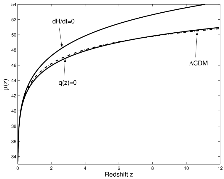
Figure 1: The distance modulus $\mu(z)$. The dash-dotted line corresponds to the $\Lambda$CDM model with $\Omega_{m}=0.27$. The solid line corresponds to the bound from the strong energy condition.

Now we are ready to apply the upper bounds (6) to the discussion of the acceleration of the Universe. We plot these upper bounds on $\mu(z)$ in Fig. 2. The lower solid line corresponds to $q(z)=0$ and the upper solid line corresponds to $\dot{H}=0$. If the Universe always experiences decelerated expansion, then the distance modulus always stays in the shaded region. If some or all SN Ia data are outside the shaded region, it means the Universe has accelerated once in the past. On the other hand, if the Universe always experiences accelerated expansion, then the distance modulus always stays above the lower solid line. If all the SN Ia data are inside the shaded region, it means that the Universe has once experienced decelerated expansion, but it does not mean that the Universe has never accelerated. Therefore, we can see the evidence of acceleration from the distance modulus graph directly without invoking any cosmological model or any statistical analysis. The ESSENCE SN Ia data riess06 is used to show the evidence of acceleration. In Fig. 2, we show all the ESSENCE SN Ia data with $1\sigma$ error bars. The binned ESSENCE SN Ia data is shown in Fig. 3. In Fig. 4, we re-plot Fig. 2 in the redshift range $0.4\leq z\leq 1.3$. From Figs. 2- 4, it is evident that the Universe had accelerated in the past because there are substantial numbers of SN Ia lying outside the shaded region. We would like to stress that this conclusion is totally model independent. There is no model or parametrization involved in this conclusion. The assumptions we use are Einstein’s general relativity and the Robertson-Walker metric. For comparison, we also show the model $\Omega_{m}=1$ (the dashed line) and the $\Lambda$CDM model with $\Omega_{m}=0.27\pm 0.04$ (the dash dotted line); the $1\sigma$ error is shown in the shaded region around the dashed dotted line. Note that due to integration effect, even if some high $z$ SN Ia data are outside the shaded region, it does not mean that we see evidence of acceleration in the high $z$ region. It is wrong to conclude that the strong energy condition is violated in the high redshift region $z>1$. The correct conclusion is that the strong energy condition was once violated in the past.

We may wonder about the low $z$ data. From Fig. 2, we see that $\mu(z)$ is almost independent of any model. In fact, to the lowest order, $d_{L}(z)=H_{0}z$. Because the data are given with arbitrary distance normalization, so $H_{0}$ for this data can be determined from the nearby supernova data $z\leq 0.1$ with $d_{L}(z)=H_{0}z$. We find that $H_{0}=64.04$ and this value is used. Because $\mu(z)$ is almost degenerate in the low redshift region $z\leq 0.1$, a current property of dark energy like $w_{0}$ is not well determined from the SN Ia data. This was discussed in gong07 ; astier01 ; huterer ; weller ; alam ; gong04 ; gong05 with the help of the sweet spot of $w(z)$.

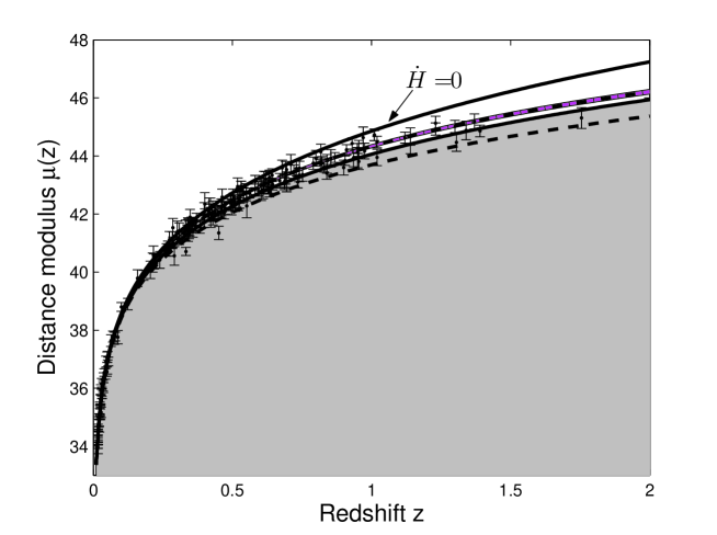
Figure 2: The distance modulus $\mu(z)$. The solid lines denote the bounds from the energy conditions. The dashed line corresponds to the model $\Omega_{m}=1$ and the dash-dotted line is for the $\Lambda$CDM model.

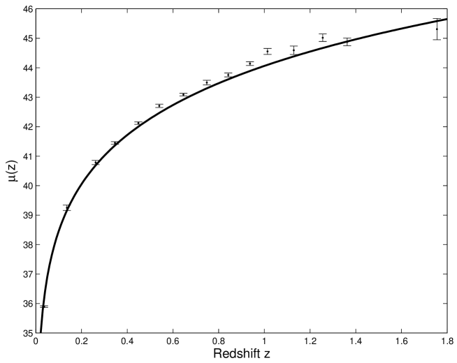
Figure 3: The distance modulus $\mu(z)$. The solid line corresponds to $q(z)=0$. The SN Ia data is the binned ESSENCE data with $1\sigma$ error.

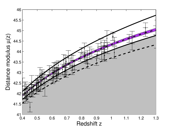
Figure 4: The distance modulus $\mu(z)$ in the redshift region 0.4-1.3.

III Properties of dark energy

In this section, we use a simple example to show that the choice of $w_{0}$ is not a good one for exploring the property of dark energy. We use two models to show this. The two models have the same behaviors at $z>z_{c}$ and different behaviors at $z\leq z_{c}$, where $z_{c}$ is arbitrary and small. The first dark energy parametrization that we consider is lind

$$w(z)=w_{0}+\frac{w_{a}z}{1+z}.$$ (7)

The dimensionless dark energy density is

$$\Omega_{DE}(z)=\Omega_{DE0}(1+z)^{3(1+w_{0}+w_{a})}\exp[-3w_{a}z/(1+z)].$$ (8)

By fitting this model to the essence data riess06 , we find that $\chi^{2}=195.07$, $\Omega_{m}=0.35^{+0.14}_{-0.35}$, $w_{0}=-1.11^{+1.45}_{-0.93}$ and $w_{a}=-1.17^{+4.61}_{-17.48}$. If we fix $\Omega_{m}=0.27$, then the best fit results are $\chi^{2}=195.17$, $w_{0}=-1.12\pm 0.44$ and $w_{a}=0.59^{+2.32}_{-2.54}$. From the Fisher matrix estimation, we find the sweet spot is around $z=0.21$. If we fix $\Omega_{m}=0.27$ and $w_{a}=0.59$, then $w_{0}=-1.12^{+0.09}_{-0.10}$ (1$\sigma$) ${}^{+0.17}_{-0.20}$ ($2\sigma$) ${}^{+0.25}_{-0.31}$ ($3\sigma$). We plot the distance modulus for this model with $\Omega_{m}=0.27$, $w_{0}=-1.12$ and $w_{a}=0.59$ in Fig. 5.

The second dark energy parametrization that we consider is

$$w(z)=\begin{cases}w_{1}+w_{2}z,&z\leq z_{c},\\ w_{0}+w_{a}z/(1+z),&z>z_{c},\end{cases}$$ (9)

where $w_{2}=(w_{0}-w_{1})/z_{c}+w_{a}/(1+z_{c})$. The dimensionless dark energy density is

$$\Omega_{DE}(z)=\begin{cases}\Omega_{DE0}(1+z)^{3(1+w_{1}-w_{2})}\exp(3w_{2}z),&z\leq z_{c},\\ \Omega_{DEi}(1+z)^{3(1+w_{0}+w_{a})}\exp[-3w_{a}z/(1+z)],&z>z_{c},\end{cases}$$ (10)

where $\Omega_{DEi}=\Omega_{DE0}(1+z_{c})^{3(w_{1}-w_{2}-w_{0}-w_{a})}$ $\exp[3z_{c}(w_{2}+w_{a}/(1+z_{c}))]$. We choose $\Omega_{m}=0.27$, $w_{0}=-1.12$, $w_{a}=0.59$ and $z_{c}=0.1$. If we take $w_{1}=-2.5$, we get $\chi^{2}=197.90$. If $w_{1}=-2.0$, $\chi^{2}=196.12$. If $w_{1}=-1.5$, $\chi^{2}=195.21$. If $w_{1}=-0.5$, $\chi^{2}=196.49$. If $w_{1}=-0.4$, $\chi^{2}=196.88$. In the first model (7), we find $-1.43\leq w_{0}\leq-0.85$ at the $3\sigma$ level. However, $w_{1}=-0.4$ and $w_{1}=-2.0$ are just a little more than $1\sigma$ away from $w_{0}=-1.12$. So we conclude that $w(z=0)$ is not well constrained by the SN Ia data. The distance modulus for this model with $w_{1}=-0.4$ and $w_{1}=-2.0$ are shown in Fig. 5. In Fig. 6, we plot the differences between the model (9) and the model (7) for $w_{1}=-0.4$ and $w_{1}=-2.0$. For completeness, we also vary $z_{c}$ in the model (9) and compare the 2$\sigma$ error of $w_{1}$ with that of $w_{0}$ for different choice of $z_{c}$. We plot the result in Fig. 7. For bigger $z_{c}$, the difference becomes smaller which is consistent with the appearance of the sweet spot around $z=0.21$. At lower redshift, the models become more degenerate and the error bar of $w(z)$ becomes bigger.

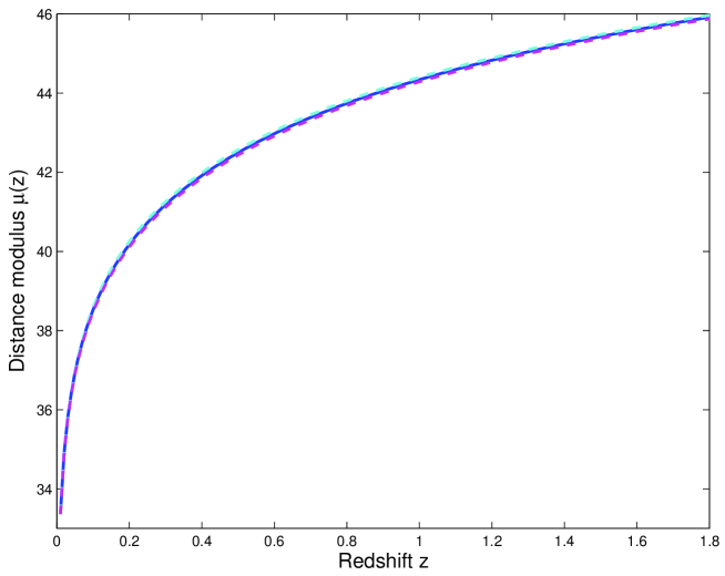
Figure 5: The distance modulus $\mu(z)$ with $\Omega_{m}=0.27$, $w_{0}=-1.12$ and $w_{a}=0.59$. The solid line is for the model (7). The dashed lines are for the model (9) with $w_{1}=-0.4$ and $w_{1}=-2$.

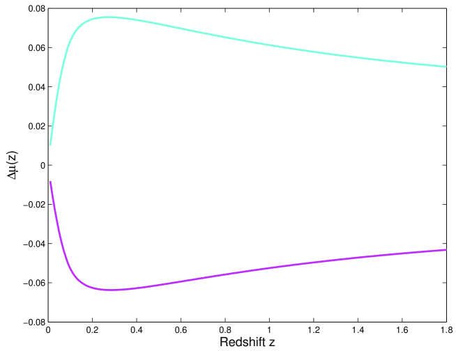
Figure 6: $\Delta\mu(z)$ between the models (7) and (9). The upper curve is for $w_{1}=-2$ and the lower curve is for $w_{1}=-0.4$.

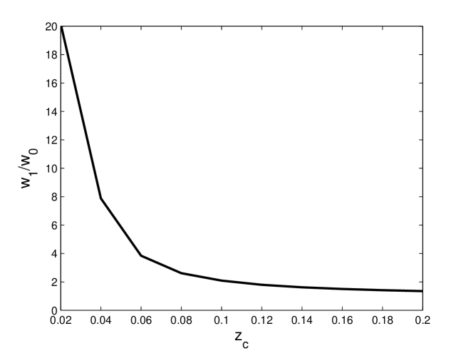
Figure 7: The 2$\sigma$ lower value of $w_{1}$ normalized by the 2$\sigma$ lower value of $w_{0}$ as a function of $z_{c}$.

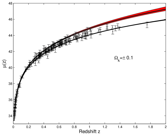
Figure 8: The upper bounds on $\mu(z)$ from the energy conditions. The solids line correspond to the flat universe $\Omega_{k}=0$. The shaded regions around these two lines correspond to $\Omega_{k}=\pm 0.1$.

IV Non-flat Universe

When $k\neq 0$, the luminosity distance becomes

$$d_{\rm L}(z)=\frac{1+z}{H_{0}\sqrt{|\Omega_{k}|}}{\rm sinn}\left[\sqrt{|\Omega_{k}|}\int_{0}^{z}\frac{dz^{\prime}}{E(z^{\prime})}\right],$$ (11)

where ${\rm sinn}(\sqrt{|k|}x)/\sqrt{|k|}=\sin(x)$, $x$, $\sinh(x)$ if $k=1$, 0, $-1$. Substitute the lower bounds on $H(z)$ in Eqs. (3) and (4) into Eq. (11), we get upper bounds on $d_{L}(z)$. We plot the upper bounds for $\mu(z)$ in Fig. 8. In this plot, we choose $\Omega_{k}=\pm 0.1$ which satisfies the observational constraint. From Fig. 8, we see that even with $\Omega_{k}$ as large as $\pm 0.1$, it is evident that the Universe had experienced accelerated expansion.

V Discussion

The energy conditions $\rho+3p\geq 0$ and $\rho+p\geq 0$ give lower bounds (3) and (4) on the Hubble parameter $H(z)$, and upper bounds on the distance modulus. If some SN Ia data are outside the region bounded by Eq. (3), then we conclude that the Universe had experienced accelerated expansion. In other words, the distance modulus-redshift graph can be used to provide direct model independent evidence of accelerated and super-accelerated expansion. If some SN Ia data are outside the region bounded by Eq. (4), then we conclude that the Universe experienced super-accelerated expansion for a flat universe. Unlike the usual parametrization methods, there is no statistical analysis involved; all we need to do is to put the SN Ia data in the distance modulus-redshift graph and see if there are substantial numbers of SN Ia data lying outside or inside the bound given by the strong energy condition. However, this direct probe does not provide us any detailed information about the acceleration, nor the nature of dark energy. Because the luminosity distance is an integral of the Hubble parameter, the distance modulus does not give us any information about the transition from decelerated expansion to accelerated expansion. As we see from the $\Lambda$CDM model in Fig. 1, even when the Universe was experiencing decelerated expansion in the past, the distance modulus may still stay outside the bounded region for a while. Due to the same reason, the distance modulus may satisfy the lower bound when the Universe is accelerating ygaz . The interpretation of the bounds on the distance modulus is very important. These bounds provide the evidence of acceleration or deceleration only, and they gave no information on how and when the acceleration happened.

At low redshift $z\leq 0.1$, the distance modulus is almost the same for all the cosmological models. For example, the difference of the distance modulus at $z=0.1$ between the $\Omega_{m}=1$ and $\Omega_{\Lambda}=1$ models is 0.16. This is well within the current observational limit. It is even difficult for future nearby SN Ia observation to reach limit below this uncertainty due to intrinsic systematics and peculiar velocity dispersion. Therefore, the property of dark energy at low redshift cannot be well constrained. This point was discussed in gong07 ; astier01 ; huterer ; weller ; alam ; gong04 ; gong05 with the help of the sweet spot of $w(z)$. We use two dark energy models which are identical at $z>0.1$ and differ at $z\leq 0.1$ to further support this argument. From the model (7), we find that $-1.43\leq w_{0}\leq-0.85$ at the $3\sigma$ level. At a little more than $1\sigma$ level, we get $-2.0\leq w_{0}\leq-0.4$ for the model (9). So the $w_{0}$-$w_{a}$ parameterizations do not provide definite information about the nature of dark energy.

In conclusion, the energy conditions provide direct and model independent evidence of the accelerated expansion. The bounds on the distance modulus also provide some directions for the future SN Ia observations. Unfortunately, the method has some serious limitations. It does not provide any detailed information about the acceleration and the nature of dark energy.

- (1) A.G. Riess et al., Astron. J. 116, 1009 (1998); S. Perlmutter et al., Astrophy. J. 517, 565 (1999).
- (2) A.G. Riess et al., Astrophys. J. 607, 665 (2004).
- (3) P. Astier et al., Astron. and Astrophys. 447, 31 (2006).
- (4) A.G. Riess et al., astro-ph/0611572; W.M. Wood-Vasey et al., astro-ph/0701041; T.M. Davis et al., astro-ph/0701510.
- (5) D.N. Spergel et al., Astrophys. J. Suppl. 170, 377 (2007).
- (6) D.J. Eisenstein et al., Astrophys. J. 633, 560 (2005).
- (7) V. Sahni and A. A. Starobinsky, Int. J. Mod. Phys. D 9, 373 (2000); T. Padmanabhan, Phys. Rep. 380, 235 (2003); P.J.E. Peebles and B. Ratra, Rev. Mod. Phys. 75, 559 (2003); V. Sahni, The Physics of the Early Universe, edited by E. Papantonopoulos (Springer, New York 2005), P. 141; T. Padmanabhan, Proc. of the 29th Int. Cosmic Ray Conf. 10, 47 (2005); E.J. Copeland, M. Sami and S. Tsujikawa, Int. J. Mod. Phys. D 15, 1753 (2006).
- (8) J.-M. Virey et al., Phys. Rev. D 72, 061302(R) (2005).
- (9) C.A. Shapiro and M.S. Turner, Astrophys. J. 649, 563 (2006).
- (10) Y.G. Gong and A. Wang, Phys. Rev. D 73, 083506 (2006).
- (11) Y.G. Gong and A. Wang, Phys. Rev. D 75, 043520 (2007).
- (12) P. Astier, Phys. Lett. B 500, 8 (2001).
- (13) D. Huterer and M.S. Turner, Phys. Rev. D 64, 123527 (2001).
- (14) J. Weller and A. Albrecht, Phys. Rev. D 65, 103512 (2002).
- (15) U. Alam, V. Sahni, T.D. Saini and A.A. Starobinsky, Mon. Not. Roy. Astron. Soc. 354, 275 (2004).
- (16) Y.G. Gong, Class. Quantum Grav. 22, 2121 (2005).
- (17) Y.G. Gong and Y.Z. Zhang, Phys. Rev. D 72, 043518 (2005).
- (18) M. Chevallier and D. Polarski, Int. J. Mod. Phys. D 10, 213 (2001); E.V. Linder, Phys. Rev. Lett. 90, 091301 (2003).
- (19) H.K. Jassal, J.S. Bagla and T. Padmanabhan, Mon. Not. Roy. Astron. Soc. 356, L11 (2005).
- (20) T.R. Choudhury and T. Padmanabhan, Astron. Astrophys. 429, 807 (2005).
- (21) J. Weller and A. Albrecht, Phys. Rev. Lett. 86, 1939 (2001); D. Huterer and G. Starkman, ibid. 90, 031301 (2003).
- (22) G. Efstathiou, Mon. Not. Roy. Astron. Soc. 310, 842 (1999); B.F. Gerke and G. Efstathiou, ibid. 335, 33 (2002); P.S. Corasaniti and E.J. Copeland, Phys. Rev. D 67, 063521 (2003); S. Lee, ibid. 71, 123528 (2005); K. Ichikawa and T. Takahashi, ibid. 73, 083526 (2006); J. Cosmol. Astropart. Phys. 02 (2007) 001; C. Wetterich, Phys. Lett. B 594, 17 (2004).
- (23) U. Alam, V. Sahni and A.A. Starobinsky, J. Cosmol. Astropart. Phys. 06 (2004) 008; R.A. Daly and S.G. Djorgovski, Astrophys. J. 597, 9 (2003); R.A. Daly and S.G. Djorgovski, ibid. 612, 652 (2004).
- (24) J. Jönsson, A. Goobar, R. Amanullah and L. Bergström, J. Cosmol. Astropart. Phys. 09 (2004) 007; Y. Wang and P. Mukherjee, Astrophys. J. 606, 654 (2004); Y. Wang and M. Tegmark, Phys. Rev. Lett. 92, 241302 (2004); V.F. Cardone, A. Troisi and S. Capozziello, Phys. Rev. D 69, 083517 (2004); D. Huterer and A. Cooray, ibid. 71, 023506 (2005).
- (25) Y.G. Gong, Int. J. Mod. Phys. D 14, 599 (2005); M. Szydlowski and W. Czaja, Phys. Rev. D 69, 083507 (2004); ibid. 083518 (2004); M. Szydlowski, Int. J. Mod. Phys. A 20, 2443 (2005).
- (26) B. Wang, Y.G. Gong and R.-K. Su, Phys. Lett. B 605, 9 (2005).
- (27) H.K. Jassal, J.S. Bagla and T. Padmanabhan, Phys. Rev. D 72, 103503 (2005).
- (28) S. Nesseris and L. Perivolaropoulous, J. Cosmol. Astropart. Phys. 01 (2007) 018; 02 (2007) 025.
- (29) V. Berger, Y Gao and D. Marfatia, Phys. Lett. B 648, 127 (2007).
- (30) V. Sahni and A.A. Starobinsky, Int. J. Mod. Phys. D 15, 2105 (2006); U. Alam, V. Sahni and A.A. Starobinsky, J. Cosmol. Astropart. Phys. 02 (2007) 011.
- (31) H. Li et al., astro-ph/0612060; G.-Z. Zhao et al., astro-ph/0612728; X. Zhang and F.-Q. Wu, Phys. Rev. D 76, 023502 (2007); L.-I. Xu, C.-W. Zhang, B.-R. Chang and H.-Y. Liu, astro-ph/0701519; H. Wei, N.-N. Tang and S.N. Zhang, Phys. Rev. D 75, 043009 (2007).
- (32) Y. Wang and P. Mukherjee, Astrophys. J. 650, 1 (2006).
- (33) E.V. Linder and D. Huterer, Phys. Rev. D 67, 081303(R) (2003).
- (34) T.D. Saini, Mon. Not. Roy. Astron. Soc. 344, 129 (2003).
- (35) H.K. Jassal, J.S. Bagla and T. Padmanabhan, astro-ph/0601389.
- (36) S. Nesseris and L. Perivolaropoulous, Phys. Rev. D 72, 123519 (2005); P. Serra, A. Heavens and A. Melchiorri, astro-ph/0701338; C. Zunckel and R. Trotta, astro-ph/0702695; A. Shafieloo, astro-ph/0703034.
- (37) M. Visser, Phys. Rev. D 56, 7578 (1997).
- (38) J. Santos, J.S. Alcaniz and M.J. Rebouças, Phys. Rev. D 74, 067301 (2006); J. Santos, J.S. Alcaniz, N. Pires and M.J. Rebouças, astro-ph/0702728, Phys. Rev. D 75, 083523 (2007).
- (39) A.A. Sen and R.J. Scherrer, astro-ph/0703416.
- (40) Y.G. Gong and A. Wang, arXiv: 0705.0996, Phys. Lett. B 652, 63 (2007).