Air-shower simulations with and without thinning: artificial fluctuations and their suppression

Abstract

The most common way to simplify extensive Monte-Carlo simulations of air showers is to use the thinning approximation. We study its effect on the physical parameters reconstructed from simulated showers. To this end, we have created a library of showers simulated without thinning with energies from $10^{17}$ eV to $10^{18}$ eV, various zenith angles and primaries. This library is publicly available. Physically interesting applications of the showers simulated without thinning are discussed. Observables reconstructed from these showers are compared to those obtained with the thinning approximation. The amount of artificial fluctuations introduced by thinning is estimated. A simple method, multisampling, is suggested which results in a controllable suppression of artificial fluctuations and at the same time requires less demanding computational resources as compared to the usual thinning.

I Introduction

Experimental information about cosmic particles at very high energies is obtained through the study of atmospheric showers induced by these particles and is hence indirect. A necessary ingredient of these studies is therefore a good understanding of a shower initiated by a primary particle with given parameters. Since the shower development is a complicated random process, the Monte-Carlo simulations are often used to model atmospheric showers. Physical parameters are then reconstructed from the simulations and compared to real data.

At very high energies, however, the number of particles in a shower is so large that the simulations start to require unrealistic computer resources. Among several ways to simplify the problem and to reduce the computational time, the thinning approximation Hillas:1997tf is currently the most popular one. Its key idea is to track only a representative set of particles; while very efficient in calculations and providing correct values of observables on average, this method introduces artificial fluctuations because the number of tracked particles is reduced by several orders of magnitude. These artificial fluctuations mix with natural ones and therefore reduce the precision of determination of physical parameters.

The standard approach to account for natural fluctuations in the air-shower simulations is to fix all shower parameters and to simulate sufficient number of artificial showers. Technically, these showers differ by initial random seed numbers. All interactions in a simulated shower are fixed by these numbers for a given thinning level. Random variations of these numbers result in a plethora of possible interaction patterns which end up in a distribution of an observable quantity of interest calculated for the showers with exactly the same initial physical parameters. This distribution thus intends to represent intrinsic fluctuations in the shower development. Both the central value and the width of this distribution are important for physical applications.

In practice, however, the width of the distribution arises from two sources: physical fluctuations and artificial fluctuations introduced by thinning. To obtain the physical width alone, one should in principle perform simulations without thinning. This is hardly possible for the highest energies at the current level of computational techniques since one often needs to simulate thousands of events for a typical study.

The aim of the present work is to estimate the relative size of these artificial fluctuations (for the first time it is done by direct comparison of showers simulated with and without thinning) and to develop an efficient resource-saving method to suppress them in realistic calculations.

In Sec. II, we start with a description (Sec. II.1) of the standard thinning algorithm and explain why its use introduces additional fluctuations. Then, we briefly recall, in Sec. II.2, conventional approaches to avoid or suppress these fluctuations. Sec. II.3 describes the library of showers simulated without thinning for this study. This library is publicly available. Sec. III is devoted to a quantitative study of the artificial fluctuations. A new method, multisampling, which allows one to suppress efficiently these unphysical fluctuations without invoking extensive computer resources, is suggested and discussed in Sec. IV. Sec. V contains the discussion of the method and our conclusions.

II Thinning approximation and beyond

II.1 Standard thinning

The number of particles in an extended air shower (EAS), and hence the CPU time and disk space required for its full simulation, scales with the energy of the primary particle. At energies in excess of $10^{17}$ eV, the number of particles of kinetic energy above 100 MeV at the ground level exceeds $10^{8}$ and the time required to simulate such a shower at a computer with a few-GHz CPU is of order of several days. A typical vertical shower induced by a hadron of $10^{18}$ eV requires about 100 Gb of disk space and a month of CPU time. Modelling individual showers with incident energies of about $10^{20}$ eV is at the limit of realistic capabilities of modern computers; meanwhile one needs thousands of simulated showers for comparison with experimental data.

As a result of a full simulation of a shower, one obtains the list of all particles at the ground level. This information is redundant for many practical purposes. Real ground-based experiments detect only a small fraction of these particles, so for calculating average particle densities one does not need to know precise coordinates and energies of all particles. In the thinning approximation Hillas:1997tf ; Nagano:1999xk , groups of particles are replaced by effective representative particles with weights.

Let us briefly recall how the thinning approximation works (see e.g. Ref. Kobal for a detailed discussion). Denote the primary energy by $E_{0}$ and introduce a parameter $\epsilon$ called the thinning level. For each subsequent interaction, consider the energies $E_{j}$ of the secondary particles created in this interaction. If the condition

$$\sum E_{j}<\epsilon E_{0}$$ (1)

is satisfied, then the method prescribes to keep one of the secondary particles and to discard the others. The probability to keep the $i$th particle $p_{i}$ is proportional to its energy,

$$p_{i}=E_{i}/\sum_{j}E_{j}.$$

To the selected particle, the weight $w_{i}=w_{0}/p_{i}$ is assigned, where $w_{0}$ is the weight of the initial particle of this interaction ($w_{0}=1$ for the particle which initiated the shower).

If the condition (1) is not satisfied, then the so-called statistical thinning operates: among the secondary particles, a subsample of ones with energies $E_{j^{\prime}}<\epsilon E_{0}$ is considered and (one or more) effective particles are selected with probabilities

$$p_{i^{\prime}}=\frac{E_{i^{\prime}}}{\min(\epsilon E_{0},\sum_{j^{\prime}}E_{j^{\prime}})}~{}.$$

These particles, to which the weights $w_{i^{\prime}}=w_{0}/p_{i^{\prime}}$ are assigned, are kept for further simulations together with original particles which have had energies $E_{j^{\prime}}>\epsilon E_{0}$.

For useful values of $\epsilon$, the number of particles tracked is reduced by a factor of $10^{3}$ – $10^{6}$. For a random process, this change in the number of particles (and consequently, in the number of interactions) results in the increase of fluctuations compared to the fully simulated process. This means that a part of fluctuations in the development of a shower simulated with thinning is artificial, that is it is present neither in the full shower simulated with $\epsilon=0$ nor in a real EAS. For a number of applications, these fluctuations are undesirable and should be suppressed or at least brought under control.

II.2 Standard methods to suppress fluctuations

In the framework of the thinning method, the fluctuations are effectively suppressed by introducing the upper limit on the weight factor $w_{i}$ Kobal . The number of “real” particles tracked is thus enlarged. Maximal weights for hadrons and for electromagnetic particles may be assigned in different ways. For a given problem, the optimal values of the maximal weights may be found in order to minimise the ratio of the size of artificial fluctuations to the computational time. In what follows, when we refer to the thinning with weights limitation, we will use the maximal weights optimised in Ref. Kobal for the calculation of the particle density.

The optimal values of parameters of thinning procedure may depend on the interaction models adopted in simulations for a given problem. In principle, the weights should be optimized for each combination of the models (which are updated every few years) and for each particular task (different observables, primaries, energies, etc.). However, this optimization requires a dedicated time consuming study in each case. We suggest another approach to the problem in Sec. IV.

II.3 A library of showers simulated without thinning

We have performed simulations of air showers without thinning by making use of the CORSIKA simulation code Heck:1998vt . For different showers, we have used QGSJET 01C Kalmykov:1997te and QGSJET II-03 Ostapchenko:2004ss as high-energy and GHEISHA 2002d Fesefeldt:1985yw as low-energy hadronic interaction models. Currently, the library contains about 40 showers induced by primary protons, gamma-rays and iron nuclei with energies between $10^{17}$ eV and $10^{18}$ eV and zenith angles between $0^{\circ}$ and $45^{\circ}$. The showers have been simulated for the observational conditions (atmospheric depth and geomagnetic field) of either AGASA Chiba:1991nf or the Telescope Array Kakimoto:2003ds experiments. The shower library Rubtsov:GZK40 is publicly available at http://livni.inr.ac.ru. Detailed information about input parameters used for the simulation of each shower is available from the library website together with full output files. The access to the data files is provided freely upon request. For users not familiar with the CORSIKA output format, a ”Datafile reading programming manual” is given, containing a working example in C++. Free access to the computational resources of the server is provided to avoid lengthy copying of the output files (some of which exceed 100 Gb in size). An access request form along with conditions of the usage of the library are available from the library website.

Given the amount of computing resources required for simulation, each shower simulated without thinning is valuable. We hope that the open library would be useful in studies of various physical problems, notably facing the improved precision of modern experiments which often exceeds the precision of simulations. The library is being continuously extended; we plan to supplement it with showers of higher energies in the future.

III Size of artificial fluctuations due to thinning

III.1 Shower-by-shower comparison

With a library of showers simulated without thinning, the comparison of the observables reconstructed from showers with and without thinning is possible. This allows one to estimate the effect of the approximation. To do that, for each shower without thinning ($\epsilon=0$) we have simulated a number of showers with different thinning levels ($\epsilon\neq 0$). All initial parameters (including the random seed numbers) were kept the same as in the $\epsilon=0$ simulation, which enabled us to reproduce exactly the same first interaction in the entire set of showers. Three important observables — the signal density at 600 m from the shower axis $S(600)$, the muon density at 1000 m from the axis $\rho_{\mu}(1000)$, and the depth of the maximal shower development $X_{\rm max}$ — were reconstructed for each of the showers following the data-processing operation adopted by the AGASA experiment. The detector response was calculated with the help of GEANT simulations in Ref. Sakaki . $S(600)$ and $\rho_{\mu}(1000)$ were obtained by fitting the corresponding density at the ground level with empirical formulae Yoshida:1994jf ; Hayashida:1995tu . For fitting purpose the density was binned into 50m-width rings centered at the shower axis. $X_{\rm max}$ was obtained by fitting the longitudinal shower profile with the empirical Gaisser-Hillas curve GaisserHillas (incorporated into CORSIKA). This procedure was repeated for all showers in the Livni library with the results similar to those shown in Figs. 1–3.

Figure 1

Figure 1: Distribution of $S(600)/S(600)_{\rm no~{}thinning}$, where $S(600)$ is reconstructed from 500 showers simulated with $\epsilon=10^{-4}$ and the same random seed as the corresponding $\epsilon=0$ shower, for three different random seeds (three histograms). The three showers are all vertical, induced by $10^{18}$ eV protons at the AGASA location.

shows the distribution of the reconstructed $S(600)$ for showers with thinning simulated with the same initial random seed (and thus the same first interaction) as three representative $\epsilon=0$ Livni showers. Though quite wide for $\epsilon=10^{-4}$ thinning, the distributions of $S(600)/S(600)_{\rm no~{}thinning}$ are well centered at unity.

The distribution of the mean values of $S(600)/S(600)_{\rm no~{}thinning}$ for the ensembles of the thinned showers is presented in Fig. 2

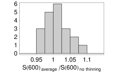
Figure 2: Distribution of $S(600)_{\rm average}/S(600)_{\rm no~{}thinning}$, where $S(600)_{\rm average}$ is the average of the reconstructed $S(600)$ over a sample of 500 showers simulated with $\epsilon=10^{-4}$ and the same random seed as the corresponding $\epsilon=0$ shower, for 20 different random seeds. The 20 showers are all vertical, induced by $10^{17}$ eV protons at the Telescope-Array location.

for a uniform sample of twenty different $\epsilon=0$ showers. For each of them, 500 showers with $\epsilon=10^{-4}$ were simulated with the same first interaction as the corresponding $\epsilon=0$ shower. The values of the observable averaged over 500 thinned showers approximate the “exact” $S(600)_{\rm no~{}thinning}$ with the accuracy of about $3\%$, which is consistent with the level of statistical fluctuations, $1/\sqrt{500}\sim 4\%$. We have found the same distributions for other observables considered, $\rho_{\mu}(1000)$ and $X_{\rm max}$. The important conclusion is that for the first time, the usual assumption that thinning does not introduce systematic errors in the reconstructed observables has been checked by explicit comparison of $\epsilon=0$ shower and averaged $\epsilon\neq 0$ showers, at least for energies up to $10^{18}$ eV, observables $S(600)$, $\rho_{\mu}(1000)$ and $X_{\rm max}$, and proton, photon and iron primaries.

The spread of observables reconstructed from thinned showers depends on the thinning level $\epsilon$. It is not the width of the distribution but the average deviation of the observables from those of an $\epsilon=0$ shower which is the most interesting for practical purposes. This quantity is plotted in Fig. 3

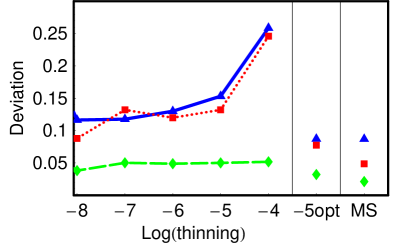
Figure 3: RMS deviations from unity of $S(600)/S(600)_{\rm no~{}thinning}$ (blue triangles and thick blue line), $\rho_{\mu}(1000)/\rho_{\mu}(1000)_{\rm no~{}thinning}$ (red boxes and red dotted line), $X_{\rm max}/X_{\rm max,~{}no~{}thinning}$ (green diamonds and green dashed line), where quantities with subscript “no thinning” are reconstructed from a $10^{18}$ eV proton shower with zenith angle 45^∘, simulated without thinning for the AGASA observational conditions, while the rest of quantities are reconstructed from large samples of showers simulated with various thinning levels for the same input parameters and the same initial random seed. “$-5$ opt” denotes $\epsilon=10^{-5}$ with weights limitation; “MS” denotes multisampling ($20\times 10^{-4}$) discussed in Sec. IV.

for a typical shower from the Livni library.

We note in passing that, technically, to study the spread at a given $\epsilon$ with CORSIKA, one has to simulate showers with slightly different thinning levels (otherwise they all would be absolutely identical, given a fixed random seed). For instance, to obtain the points corresponding to $\epsilon=10^{-5}$ in Fig. 3, we have simulated 500 showers with different thinning levels in the interval $0.99\cdot 10^{-5}<\epsilon<1.01\cdot 10^{-5}$.

III.2 Distributions of showers

In most cases one is not interested in details of a particular realization of a shower; it is the ensemble of simulated showers with fixed initial parameters but varied random seeds which is compared to the real data. The study of Sec. III.1 does not help seriously to estimate the effect of thinning on these distributions of parameters because the size of fluctuations seen, e.g., in Fig. 3 is determined by a combination of artificial fluctuations and a part of real ones: the random seed together with initial conditions fixes the first interaction, but different thinning levels introduce variations in other interactions and effectively change the simulation of the entire shower development.

To estimate the effect of thinning on the distribution of observables, we have simulated samples of showers with fixed initial conditions but different random seeds for various thinning levels, including $\epsilon=0$. We have considered samples of $E=10^{17}$ eV vertical proton-induced showers consisting of 20 showers with $\epsilon=0$, 100 showers with $\epsilon=10^{-5}$, 100 showers with $\epsilon=10^{-5}$ and weight limitation, 100 showers with $\epsilon=10^{-4}$ and 100 showers with $\epsilon=10^{-4}$ and weight limitation.

The simulations have been performed using QGSJET II and GHEISHA as hadronic interaction models, for the observational conditions of the Telescope Array experiment. The distributions of $S(600)$, $\rho_{\mu}(1000)$ and $X_{\rm max}$ have been reconstructed with statistical fluctuations (originated from the limited number $n$ of showers in the samples) of about $1/\sqrt{n}$, that is, about 23% for $\epsilon=0$ showers and about 10% for the other samples. Figure 4

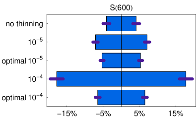
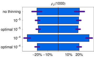
Figure 4: Width of the $S(600)$ distribution (upper panel) and $\rho_{\mu}(1000)$ distribution (lower panel) for $10^{17}$ eV vertical proton showers simulated with and without thinning for the Telescope Array observational conditions. Statistical error bars are due to a limited number of simulated showers.

illustrates the widths of the distributions obtained at different $\epsilon$. Artificial fluctuations in $S(600)$ and $\rho_{\mu}(1000)$ caused by thinning are clearly seen by comparing $\epsilon=10^{-4}$ case with others (for $X_{\rm max}$ the artificial fluctuations are quite small). We note that, for a given $\epsilon$, the fluctuations should be larger at high energy since the multiplicity of hadronic interactions grows with energy and thinning starts to operate earlier in the shower affecting the first few interactions which determine the fluctuations. For many practical purposes, these artificial fluctuations should be efficiently suppressed.

IV Multisampling: an economical method to suppress artificial fluctuations

From the results of the previous section, we conclude that the use of thinning is well motivated when one is interested in the reconstruction of the central values of fluctuating observables (the most important application is e.g. to establish a relation between, say, $S(600)$ and energy for a given experimental setup). On the other hand, thinning may limit the precision of composition studies, where the observed value of some quantity is compared to the simulated distributions of the same quantity for different primaries, and the width of these distributions is of crucial importance (see e.g. the proton–iron comparison in examples of Ref. our-composition ).

As it has been pointed out above, the effect of physical fluctuations on the distribution of an observable quantity should be, in principle, estimated by simulating a set of showers with the same physical parameters, with different random seeds and without thinning. To obtain a good approximation to this distribution, we make use of the results of Sec. III.1 (see, in particular, Figs. 1 and 2). The average of an observable over a sample of thinned showers with a fixed initial random seed approximates the value of the same observable for an $\epsilon=0$ shower with the same random seed with a good accuracy. The distribution of observables for $\epsilon=0$ showers with different random seeds is then approximated by a distribution of these approximated observables calculated for samples with random seeds varying from one sample to another but fixed inside a sample. A practical way to do this is as follows:

• instead of a single shower with $\epsilon=0$, simulate $N$ showers with some $\epsilon=\epsilon_{0}\neq 0$ and fixed random seed;

• reconstruct the observable for each of $N$ showers, average over these $N$ realizations and keep this average value which approximates the result for a single shower without thinning;

• repeat the procedure $M$ times for different random seeds to mimic a simulation of $M$ showers without thinning and to obtain the required distribution of the observable.

We will refer to this procedure as to multisampling $(N\times\epsilon_{0})$. Even for relatively large $\epsilon$, averaging over a sufficiently large number of showers ($N$) gives a good approximation to an $\epsilon_{0}=0$ value of the observable; the larger $N$, the better the approximation. The required value of $N$ may be estimated as follows. Consider the distribution of an observable reconstructed from showers simulated with the thinning level close to $\epsilon_{0}$ for a given initial random seed. Assume that the distribution is Gaussian with the width $\sigma$ (though the qualitative conclusions do not depend on the exact form of the distribution, we note that, in practice, it is indeed very close to Gaussian ST:GZK40 ); then one needs $N$ measurements to know the mean value with the precision $\sim\sigma/\sqrt{N}$. Numerical results for the Livni showers demonstrate that $(N\times\epsilon_{0})$ multisampling for $N\sim 15\dots 20$ and $\epsilon_{0}\sim 10^{-4}$ results in the precision of $3\div 4\%$ in the reconstruction of $S(600)$, $\rho_{\mu}(1000)$ and $X_{\rm max}$ of the original $\epsilon=0$ showers. The distributions of parameters reconstructed from showers without thinning are consistent (within statistical errors) with those extracted by making use of multisampling. The distributions of $S(600)$ are presented in Fig. 5.

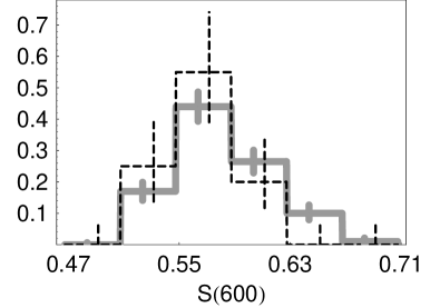
Figure 5: Normalized distributions of the reconstructed $S(600)$ (in VEM/m²): dashed line, 20 showers without thinning; solid line, 500 showers with $(20\times 10^{-4})$ multisampling. All showers are vertical, induced by $10^{17}$ eV primary protons simulated for the conditions of the Telescope Array. Vertical error bars are due to limited statistics.

In Fig. 6

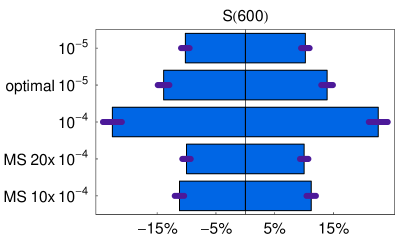
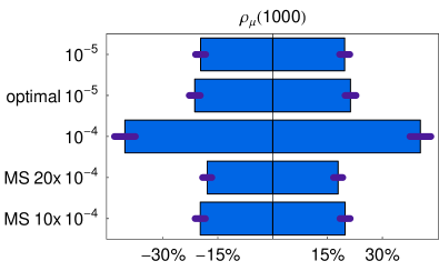
Figure 6: Width of the $S(600)$ distribution (upper panel) and $\rho_{\mu}(1000)$ distribution (lower panel) for 200 showers initiated by $5\cdot 10^{19}$ eV vertical protons simulated with thinning and with multisampling for the Telescope Array observational conditions. Statistical error bars are due to a limited number of simulated showers. The choice of maximal weights suggested in Ref. Kobal may not be optimal for this study (see the text).

we present the widths of the distributions obtained with the usual thinning and with multisampling for $E=5\cdot 10^{19}$ eV vertical proton-induced showers; the limited statistics (we used $n=200$ showers) implies the statistical uncertainty of about $1/\sqrt{n}\sim 7\%$. The gain in precision is clearly seen; for the case of $5\cdot 10^{19}$ eV the multisampled distribution (which is expected to mimic the $\epsilon=0$ distribution with a good accuracy) allows us to estimate the size of purely artificial fluctuations caused by thinning. For instance, for $\epsilon=10^{-5}$ with weights limitations, these fluctuations remain at the level of $\gtrsim 10\%$ for $S(600)$ and of $\gtrsim 12\%$ for $\rho_{\mu}(1000)$. Let us note in passing that, for this particular simulation ($5\cdot 10^{19}$ eV vertical protons at the Telescope Array location) and for our choice of hadronic models (QGSJET II and GHEISHA), the choice of maximal weights suggested in Ref. Kobal may not be optimal.

Let us compare now the computer resources needed for calculations with the standard thinning (with and without weights limitations) and with multisampling.

The disk space scales as the number of simulated particles; Fig. 7

Figure 7: The size of the CORSIKA output file for different thinning levels and procedures (a $10^{18}$ eV proton shower with zenith angle of $45^{\circ}$, AGASA observational conditions).

illustrates this fact. We see that the multisampling ($20\times 10^{-4}$) saves the disk space compared to $\epsilon=10^{-5}$ with weights limitation, giving at the same time gain in the precision of simulations.

The CPU time is very sensitive to the choice of the hadronic interaction model: since thinning starts to work when the number of particles is large enough, the first few interactions are simulated in full even for relatively large $\epsilon$. If the high-energy model is slow, then the effect of multisampling on the computational time is not so pronounced. By variations of the hadronic interaction models, we have estimated the average time consumed by QGSJET II, SYBILL, FLUKA and GHEISHA for simulations of showers at energies $10^{17}$ eV and $5\cdot 10^{19}$ eV. For $5\cdot 10^{19}$ eV vertical proton showers, ($20\times 10^{-4}$) multisampling is about 5 times faster than $10^{-5}$ thinning with weights limitation for SYBILL while for (very slow) QGSJET II, both take roughly the same time. A way to change the multisampling procedure in order to gain in the CPU time for any hadronic model is discussed below in Sec. V.

V Discussion and conclusions

A library of atmospheric showers has been simulated without the thinning approximation. The showers have been used for a quantitative direct study of the effect of thinning on the reconstruction of signal ($S$) and muon $(\rho_{\mu}$) densities at the ground level as well as on the depth $X_{\rm max}$ of the maximal shower development. We demonstrate that thinning does not introduce systematic shifts into these observables, as was conjectured but never explicitly checked. We estimate the size of artificial fluctuations which appear due to the reduction of the number of particles in the framework of the thinning approximation; these unphysical fluctuations may affect the precision, e.g., of the composition studies. For instance, at the energies of $5\cdot 10^{19}$ eV for vertical proton primaries, artificial fluctuations are about 10% in the signal density at 600 m and about 12% in the muon density at 1000 m for $\epsilon=10^{-5}$ thinning with weight limitations. An effective method to suppress these artificial fluctuations, multisampling, is suggested and studied. The method does not invoke any changes in simulation codes; only parameters of, say, the CORSIKA input are affected. Compared to the $10^{-5}$ thinning with weights limitations, it gives a similar precision but allows one to gain an order-of-magnitude decrease in the required disk space. Gain in the CPU time depends on the speed of the high-energy interaction model: it is of order $5\div 10$ for fast ones (SYBILL) and of order 1 for slow ones (QGSJET II).

A way to change the multisampling procedure in order to further improve the gain in the CPU time is to simulate the high-energy part of a shower once for each initial random seed while having the low-energy part multisampled. The multisampling procedure described above is a particular case of such improved procedure with a high-energy part restricted to the first interaction only. We would expect the modification to make it possible to conserve the physical fluctuations in the second and several following interactions and will allow for an order-of-magnitude improvement in the computational time for any hadronic model. However, it would require (simple) changes in the simulation codes thus loosing an important advantage of the multisampling discussed above: to implement the latter, one operates with the standard simulation code (e.g., CORSIKA) without any modifications. This minimal change is to add the option to start simulations from a predefined set of the primary particles.

We are indebted to T.I. Rashba and V.A. Rubakov for helpful discussions. This work was supported in part by the INTAS grant 03-51-5112, by the Russian Foundation of Basic Research grants 07-02-00820, 05-02-17363 (DG and GR), by the grants of the President of the Russian Federation NS-7293.2006.2 (government contract 02.445.11.7370; DG, GR and ST) and MK-2974.2006.2 (DG) and by the Russian Science Support Foundation (ST). Numerical part of the work was performed at the computer cluster of the Theory Division of INR RAS. Our library of showers without thinning is publicly available at http://livni.inr.ac.ru.

References

- (1) L. G. Dedenko, Can. J. Phys. 46, 178 (1968).
- (2) A. M. Hillas, Nucl. Phys. Proc. Suppl. 52B, 29 (1997).
- (3) M. Nagano, D. Heck, K. Shinozaki, N. Inoue and J. Knapp, Astropart. Phys. 13, 277 (2000).
- (4) M. Kobal, Astropart. Phys. 15, 259 (2001).
- (5) D. Heck, G. Schatz, T. Thouw, J. Knapp and J. N. Capdevielle, “CORSIKA: A Monte Carlo code to simulate extensive air showers,” FZKA-6019.
- (6) N. N. Kalmykov, S. S. Ostapchenko and A. I. Pavlov, Nucl. Phys. Proc. Suppl. 52B, 17 (1997).
- (7) S. Ostapchenko, Nucl. Phys. Proc. Suppl. 151, 143 (2006).
- (8) H. Fesefeldt, “The Simulation Of Hadronic Showers: Physics And Applications,” CERN-DD-EE-80-2.
- (9) N. Chiba et al., Nucl. Instrum. Meth. A 311, 338 (1992).
- (10) F. Kakimoto et al. [TA Collaboration], Proc. 28th ICRC, Tsukuba, 2003.
- (11) G. I. Rubtsov, Talk given at the 3rd International Workshop on the highest energy cosmic rays and their sources: Forty years of the GZK problem, http://www.inr.ac.ru/~st/GZK-40_program.html
- (12) N. Sakaki et al., Proc. 27th ICRC, Hamburg, 2001, 1, 333.
- (13) S. Yoshida et al., J. Phys. G 20, 651 (1994).
- (14) N. Hayashida et al. [AGASA Collaboration], J. Phys. G 21, 1101 (1995).
- (15) T. K. Gaisser and A. M. Hillas, Proc. 15th ICRC, Plovdiv 8, 353 (1977).
- (16) D. S. Gorbunov, G. I. Rubtsov and S. V. Troitsky, arXiv:astro-ph/0606442.
- (17) S. V. Troitsky, Talk given at the 3rd International Workshop on the highest energy cosmic rays and their sources: Forty years of the GZK problem, http://www.inr.ac.ru/~st/GZK-40_program.html