Resonances in Barred Galaxies

Abstract

The inner parts of many spiral galaxies are dominated by bars. These are strong non-axisymmetric features which significantly affect orbits of stars and dark matter particles. One of the main effects is the dynamical resonances between galactic material and the bar. We detect and characterize these resonances in N-body models of barred galaxies by measuring angular and radial frequencies of individual orbits. We found narrow peaks in the distribution of orbital frequencies with each peak corresponding to a specific resonance. We found five different resonances in the stellar disk and two in the dark matter. The corotation resonance and the inner and outer Lindblad resonances are the most populated. The spatial distributions of particles near resonances are wide. For example, the inner Lindblad resonance is not localized at a given radius. Particles near this resonance are mainly distributed along the bar and span a wide range of radii. On the other hand, particles near the corotation resonance are distributed in two broad areas around the two stable Lagrange points. The distribution resembles a wide ring at the corotation radius. Resonances capture disk and halo material in near-resonant orbits. Our analysis of orbits in both N-body simulations and in simple analytical models indicates that resonances tend to prevent the dynamical evolution of this trapped material. Only if the bar evolves as a whole, resonances drift through the phase space. In this case particles anchored near resonant orbits track the resonance shift and evolve. The criteria to ensure a correct resonant behavior discussed in Weinberg & Katz (2007a) can be achieved with few millions particles because the regions of trapped orbits near resonances are large and evolving.

1 Introduction

It is often assumed that the stellar disk in spiral galaxies can be modeled as an axisymmetric system. Departures from this symmetry are usually treated as weak non-axisymmetric perturbations, like spiral arms (Binney & Tremaine, 1987). However, many spiral galaxies show strong non-axisymmetric features such as central bars. In fact, galaxies with strong bars are very common objects in the Universe. They account for 65 per cent of bright spiral galaxies (Eskridge et al., 2000). Barred galaxies can not be modeled as nearly axisymmetric systems because the dynamics of these galaxies is dominated by a strong bar which rotates around the center. The bar interacts with galactic material and distorts galactic orbits. In particular, some galactic orbits experience dynamical resonances with the bar. The motion in these orbits is coupled with the rotation of the bar: resonant orbits are closed orbits in the reference frame which rotates with the bar. In this frame, the bar is stationary and a resonant orbit can periodically reach the same position with respect to the bar. A resonant orbit is therefore a periodic orbit in this reference frame and its dynamical frequencies are commensurable (Lichtenberg & Lieberman, 1983).

The motion of a star in a galaxy could be described by oscillations in three dimensions: radial oscillation, an oscillation perpendicular to the galactic plane, and an angular oscillation or rotation around the galactic center. In general, these oscillations could be described by three instantaneous orbital frequencies: a radial frequency $\kappa$, a vertical frequency $\nu$ and angular frequency $\Omega$. The case of a nearly circular orbit in an axisymmetric potential is especially easy to understand and to study analytically using the epicycle approximation (Binney & Tremaine, 1987). However, a general orbit in the gravitational potential of a galaxy is not a nearly circular orbit. This is especially true for barred galaxies where the radial oscillations are not small and orbits can be very elongated. In barred galaxies orbital frequencies may differ significantly from the frequencies in the epicycle approximation.

A resonance happens if the dynamical frequencies of an orbit and the angular frequency of the rotation of the bar, $\Omega_{B}$, satisfy the following relationship of commensurability:

$$\mathbf{l}\cdot\mathbf{\Omega}=m_{B}\Omega_{B}$$ (1)

where l=$(l,m,n)$ is a vector of integers, $\mathbf{\Omega}$ is a vector of frequencies, $\mathbf{\Omega}=(\kappa,\Omega,\nu)$ and $m_{B}$ is also a integer. We mostly will be interested in cases with $m_{B}=m$ and in motions close to the galactic plane: $n=0$. So, the resonant condition is reduced to

$$l\kappa+m(\Omega-\Omega_{B})=0$$ (2)

Thus, each planar resonance is described by a pair of integers, ($l$:$m$). A resonant ($l$:$m$) orbit is closed after $l$ revolutions around the center and $m$ radial oscillations in the reference frame which rotates with the bar. Table 1 summarizes several examples of these resonances.

One important example is the corotation resonance (CR), $\Omega=\Omega_{B}$. A star in a resonant orbit of CR rotates around the galaxy center with a speed equal to the rotation speed of the bar. Thus, it does not move in the rotating frame. Other important resonances are the inner and outer Lindblad resonances. As it seems from the rotating frame, a star in one of these resonant orbits makes two radial oscillations during one angular revolution. The resonant orbit has therefore an ellipsoidal shape. The inner Lindblad resonance (ILR) corresponds to the (-1,2) resonance. In this case, the star rotates faster than the bar, $\Omega>\Omega_{B}$. The opposite case, $\Omega<\Omega_{B}$, corresponds to the (1:2) resonance, which is the outer Lindblad resonance (OLR).

Table 1: Examples of resonances

Name    $l$		$m$	$n$	$\frac{\Omega-\Omega_{B}}{\kappa}$
CR	0	1	0	0
ILR	-1	2	0	0.5
OLR	1	2	0	-0.5
UHR	-1	4	0	-0.25

Significant effort have been made to study motions near resonances in astrophysical systems as well as in plasma physics and in Solar system dynamics (Chirikov, 1960; Lynden-Bell & Kalnajs, 1972; Tremaine & Weinberg, 1984; Weinberg, 2004; Weinberg & Katz, 2007a). One important and difficult problem is the problem of small divisors or small denominators. Suppose we impose a small perturbation and study the effect of this perturbation. In the case of barred galaxies, the unperturbed case is an axisymmetric model and the perturbation is a weak bar. One may try to find a solution to this problem using perturbation series. When this is done, the solution typically has terms with denominator $\mathbf{l}\cdot\mathbf{\Omega}-m_{B}\Omega_{B}$, which goes to zero at resonance. The reason for this divergence is the breakdown of the assumption that the solution can be written as a perturbation series. It appears that correct behavior of the solution cannot be obtained in any order of the perturbation theory (Lichtenberg & Lieberman, 1983, Sec.2.2b). One may think that the perturbation theory gives qualitatively correct answer (e.g., predicts large changes in energy and angular momentum), but it fails to estimate the magnitude of the effect. Unfortunately, this is not the case: it gives wrong qualitative answers. Binney & Tremaine (1987, Chapter 3, eqs. (3-123)-(3-129) ) give an example of treatment of orbits around stable corotation resonance (Lagrange points $L_{4}$ and $L_{5}$). In this case the perturbation expansion gives a divergent amplitude (the solution linearly grows) and the correct treatment in Binney & Tremaine (1987) does not show any growth (see also Byrd, Freeman & Buta (2006)).

It is important to formulate the situation clearly because this can produce significant confusion. In mathematics the problem is often stated as the problem of perturbations: how orbits change when a perturbation is imposed. In this case one compares perturbed orbits with the same orbits before the perturbation was imposed. Significant deviations are expected to happen for unperturbed trajectories in regions of overlapping resonances of the unperturbed system (Chirikov, 1960). Yet, this is not the problem, which we deal with in barred galaxies. In this case we study only perturbed orbits: how they change with time and how they behave close to resonances of the perturbed system. In other words, we do not compare perturbed orbits with the unperturbed trajectories. By itself it is a very interesting problem: formation of bars. Yet, at this moment we focus exclusively on the evolution under the forces of bars.

This is significantly easier problem. We also simplify the situation by considering bars which do not change with time. First, we start with orbits at exact resonances: $\vec{l}\cdot\vec{\Omega}=m_{B}\Omega_{B}$. How do they evolve? The answer is simple: they do not (Lynden-Bell & Kalnajs, 1972). Orbits at exact resonances are closed in the phase-space: after some time they come to exactly the same position in space and have exactly the same velocities. Thus, they have the same angular momentum and the same energy.

Close to the resonances the situation is complex. Lynden-Bell & Kalnajs (1972) argued that there should be significant growth of perturbations in this area. Yet, this argument was based on the perturbation expansion, which is not valid near resonances. We distinguish two types of resonances: elliptic and hyperbolic (Arnold & Avez, 1968). Lagrange points $L_{4}$ and $L_{5}$ are examples of elliptic resonances: orbits oscillate and librate around those resonances and have the structure of a simple pendulum (Lichtenberg & Lieberman 1983, Sec. 2.4, Murray & Dermott 1999, Sec. 8). Hyperbolic resonances are points on intersection of separatrixes dividing domains of elliptical resonances (e.g., Lagrange points $L_{1}$ and $L_{2}$) In this paper we are mostly interested in elliptical resonances.

There is no evolution at resonant orbits for a stationary perturbation and there is no singularities at resonances. Therefore, the small divisor problem can lead to a wrong interpretation of the secular evolution near resonances and their role in barred galaxies. A more careful treatment of the motions in near-resonant orbits reveals that the Hamiltonian near a resonance can be approximated by the Hamiltonian of the one dimensional pendulum in a variable which change slowly near the resonance (Lichtenberg & Lieberman, 1983). So, the motions near every resonance can be approximated by motions of libration, separatrix and rotation around a resonant orbit. Examples of these motions near CR and ILR can be found in section 6. Circulating pendulum solutions near CR are also given by Byrd, Freeman & Buta (2006). In general, each fixed point of the pendulum corresponds to an exactly resonant orbit. As the result, each resonance has formally two different types of resonant orbits. One corresponds to the stable or elliptic fixed point, around which the near-resonant orbits librate. The other corresponds to the unstable or hyperbolic fixed point, where the separatrices intersect. In the region around the separatrix, this pendulum approximation fails. The phase-space near the separatrix is more complex that in the case of a pendulum (Voglis, Tsoutsis & Efthymiopoulos, 2006). This area may be filled with irregular or chaotic orbits and high-order resonances ($l>1$). This is usually called the resonance layer (Lichtenberg & Lieberman, 1983). As a result of all this complexity, perturbation theory is not valid at any order near resonances. Small divisors can be removed from one order in the perturbation series, but other small divisors appear in a higher order. So, the right behavior near resonances can only be studied by solving the exact solution of the equations of motions near resonances.

The phase-space near resonances is mainly populated by trapped orbits in libration around stable resonant orbits. Their exact trajectories are commonly computed in orbit theory (Contopoulos & Grosbøl, 1989; Skokøs et al., 2002). In this field, the potential of a barred galaxy is modeled by a combination of different analytical potentials, like an axisymmetric disk plus a prolate ellipsoid. Then, galactic orbits are computed numerically using this galactic model. In this way, the galactic orbital structure can be studied in detail. Resonant orbits in this case are periodic orbits in a given non-axisymmetric potential. Each stable periodic orbit is the parent of a family of non-closed orbits which remain near to this orbit at any moment (Binney & Tremaine, 1987). The dynamical frequencies of these trapped orbits oscillate around the frequencies of the resonant orbit. Therefore, their average frequencies over time should be close to the frequencies of the resonant or parent orbit.

However, orbit studies have some limitations. They can not follow the self-consistent evolution of barred galaxies. The underlying potential is fixed and does not change due to the redistribution of the orbits. In contrast, N-body models can follow the orbits and the secular evolution of barred galaxies at the same time. However, Weinberg & Katz (2007a) have derived the necessary number of particles in an N-body model which could accurately resolve the dynamics near resonances. These required numbers are well beyond the numbers used in current state-of-the-art models. So, do we have any hope to see the effects of resonances in N-body models? We argue that current N-body models can resolve the dynamics of resonances in the regime relevant for observed barred galaxies. They have strong non-axisymmetric features. In contrast, the particle number criteria of Weinberg and Katz (2007a) were derived in the regime of weak perturbations.

N-body models have been already used to study the resonant interaction between the bar and the halo of dark matter (Holley-Bockelmann et al., 2005; Colín, Valenzuela & Klypin, 2006; Athanassoula, 2002, 2003; Martinez-Valpuesta et al., 2006; Weinberg & Katz, 2007b). N-body models open the possibility to sample individual trajectories over time and extract their dynamical frequencies. This allows a better determination of resonant orbits and their dynamics. This has been done in restricted N-body experiments with a frozen non-axisymmetric potential (Holley-Bockelmann et al., 2001; Athanassoula, 2002, 2003; Martinez-Valpuesta et al., 2006). In Athanassoula (2002), the orbital frequencies were estimated using a random population of particles taken from the disk and the halo of a N-body simulation. A frozen barred potential equal to the potential of the simulation was set to rotate with the pattern speed measured in the simulation at a given moment. Each orbit was computed in this stationary potential. Finally, the dynamical frequencies of each orbit were estimated using a spectral analysis. Some of the orbits were trapped near resonant orbits in the disk and in the halo. The slowdown of the bar was linked to the lost of angular momentum of nearly resonant orbits in the inner disk. At the same time, the gain of angular momentum of the halo was linked to the gain of angular momentum of near-resonant orbits in the halo.

However, little work has been published on the detection of resonances in a fully self-consistent N-body model of a barred galaxy. The purpose of this study was to detect and characterize the resonances present in barred galaxies. This study may also find new insights into the dynamics near resonances and their role in barred galaxies. This paper is organized as follows. §2 presents the N-body models analyzed in this paper. §3 describes the methods used to measure the dynamical frequencies of the particles. §4 describes the main results on resonances in the disk and in the halo. §5 describes the capture at corotation as an example of resonant capture. §6 compares these results with an analytical galactic model. Finally, §7 is devoted to the discussion and §8 is the summary and conclusion.

Figure 1: Face-on views of the three N-body models of barred galaxies. The contours show levels of equal surface density. Their scale is logarithmic with a step of 0.5 dex. The scale is the same for all figures. The circles represent the corotation radius for each model. The model $K_{hb}$ develops a larger and slower bar than the model $D_{hs}$. The model C has a strong and massive bar.

2 The models

Table 2: Initial parameters of models

Parameter    $D_{hs}$		$K_{hb}$	C
Disk Mass ($10^{10}{\rm M}_{{}_{\mathord{\odot}}\;}$)	5.0	5.0	4.8
Total Mass ($10^{12}{\rm M}_{{}_{\mathord{\odot}}\;}$)	1.43	1.43	1.0
Disk exponential length (kpc)	2.57	3.86	2.9
Disk exponential height (kpc)	0.20	0.20	0.14
Stability parameter $Q$	1.8	1.8	1.2
Halo concentration C	17	10	19
Total number of particles ($10^{5}$)	$38.0$	$27.2$	$97.7$
Number of disk particles ($10^{5}$)	$4.60$	$2.33$	$12.9$
Particle mass ($10^{5}{\rm M}_{{}_{\mathord{\odot}}\;}$)	$1.07$	$2.14$	$0.37$
Maximum resolution (pc)	22	22	100.
Time Step ($10^{4}yrs$)	1.48	0.95	12.

2.1 Initial conditions

The initial conditions of the N-body models are described in detail in Valenzuela & Klypin (2003). The generation of the models follows the method of Hernquist (1993). The model initially has only a stellar exponential disk and a dark matter halo. No bar is initially present in the model but the system is unstable and forms a bar. The density of the stellar disk in cylindrical coordinates is approximated by the following expression:

$$\rho_{d}(R,z)=\frac{M_{d}}{4\pi z_{0}R_{d}^{2}}e^{-\frac{R}{R_{d}}}sech^{2}(z/z_{0}),$$ (3)

where $z_{0}$ is the scale height of the disk, $R_{d}$ is the exponential length and $M_{d}$ is the mass of the disk. The scale height is assumed to be initially constant through the disk. The vertical velocity dispersion $\sigma_{z}$ is given by the scale height and the surface stellar density $\Sigma$:

$$\sigma^{2}_{z}(R)=\pi Gz_{0}\Sigma(R),$$ (4)

where G is the gravitational constant. The radial velocity dispersion $\sigma_{R}$ is also related to the surface density:

$$\sigma_{R}(R)=Q\frac{3.36G\Sigma(R)}{\kappa(R)},$$ (5)

where $\kappa(R)$ is the epicycle frequency at a given radius and Q is the Toomre stability parameter, assumed constant through the disk. The rotational velocity $V_{\phi}$ and its dispersion $\sigma_{\phi}$ are computed using the asymmetric drift approximation and the epicycle approximation,

$$V_{\phi}^{2}(R) = V_{c}^{2}(R)-\sigma_{R}^{2}(R)\left(\frac{2R}{R_{d}}+\frac{\kappa^{2}(R)}{4\Omega^{2}(R)}-1\right),$$ (6)

$$\sigma_{\phi}^{2}(R) = \sigma^{2}_{R}(R)\frac{\kappa^{2}(R)}{4\Omega^{2}(R)},$$ (7)

where $V_{c}$ is the circular velocity at a given radius and $\Omega$ is the angular frequency in the epicycle approximation.

The density profile of a cosmological motivated dark matter halo is initially well approximated by the NFW profile (Navarro et al., 1997),

$$\rho_{\rm dm}(r) = \frac{\rho_{s}}{x(1+x)^{2}},\ x=r/r_{s},$$ (8)

$$M_{\rm vir} = 4\pi\rho_{s}r_{s}^{3}\left[\ln(1+C)-{C\over 1+C}\right],\ C={r_{\rm vir}\over r_{s}},$$ (9)

where $M_{\rm vir}$ and C are the virial mass and the concentration of the halo. The radial velocity dispersion of dark matter particles is related with the mass profile of the system, M(R),

$$\sigma_{R,{\rm dm}}^{2}={1\over\rho_{\rm dm}}\int_{R}^{\infty}\rho_{\rm dm}\frac{GM(R)}{R^{2}}dR.$$ (10)

Finally, the other two components of the velocity dispersion of dark matter are equal to $\sigma_{r,{\rm dm}}^{2}$, assuming an isotropic velocity distribution. This assumption remains valid in the central parts of dark matter halos (Colín et al., 2000).

2.2 Description of the models

We analyze two of the N-body models of barred galaxies described in Colín, Valenzuela & Klypin (2006). We also include the model C of Valenzuela & Klypin (2003). These three models are consistent with normal high surface brightness galaxies. The dark matter does not dominate in the models in the first two scale lengths, $R\leq 2R_{d}$ (Klypin et al., 2002). The parameters of the models are presented in Table 2. These models do not cover a large range of parameters. This is done in Colín, Valenzuela & Klypin (2006). Instead, we have selected three models with very different initial conditions. $D_{hs}$ has a more concentrated halo and a shorter disk length than $K_{hb}$. For example, the dark matter contribution to the initial circular velocity is equal to the contribution of the disk at 7 Kpc in the model $D_{hs}$ and 10 Kpc in the model $K_{hb}$. As a result, $D_{hs}$ is initially more centrally concentrated than $K_{hb}$. The disk is hot, $Q\approx 1.8$, in these two models. In contrast, the model C has a cold disk, $Q\approx 1.2$. In addition, the halo of this model has a higher concentration than the models from Colín, Valenzuela & Klypin (2006) but its exponential length is in between the values of the other two models. As a result, 6.5 Kpc is the radius in which the contribution of the halo and the disk to the initial circular velocity are equal. All these differences are reflected in the bar evolution and therefore, they are also reflected in the resonant structure. All three models develop a relatively strong bar (Fig. 1). However, the bar in the model $D_{hs}$ is shorter and rotates faster than the bar in the model $K_{hb}$. This affects strongly the resonant structure. All three models show a slow evolution in the pattern speed of the bar, $\Omega_{B}$, so it could be considered nearly constant over a period of 1-2 Gyr (Colín, Valenzuela & Klypin, 2006). This is a suitable situation for the analysis of resonances because the resonant structure is stable if $\Omega_{B}$ is constant.

2.3 The code

These simulations were performed with the Adaptive Refinement Tree (ART) N-body code (Kravtsov et al., 1997; Kravtsov, 1999). The code computes the density and gravitational potential in each cell of a uniform grid. If the number of particles in a cell exceeds a given threshold, the cell is split in 8 smaller cells. This creates the next level of a refinement mesh. The procedure is recursive. The result is a refined mesh which accurately matches high density regions with arbitrary geometry. This spatial refinement is followed by a temporal refinement. More refined regions have a shorter time step. This is necessary to follow accurately the trajectory of particles. The code was extensively tested. Additional tests on the long-term stability of equilibrium systems were performed in Valenzuela & Klypin (2003). These tests are important to study the secular evolution in barred galaxies. The results showed that the effect of two-body scattering is negligible. The relaxation time scale was roughly equal to $4.5\times 10^{4}$ Gyr for a system with 3.5 million particles.

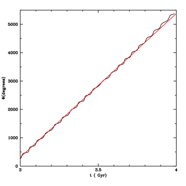
Figure 2: Example of a measurement of a radial frequency, $\kappa$, of a particle using the Fourier spectrum of its radial oscillations. The top panel shows the radius of a particle as a function of time for $K_{hb}$ and the bottom panel presents the Fourier decomposition of its radial trajectory, where P is the power spectrum. The radial frequency is measured as the maximum peak of the spectrum, $\kappa=126$ Km s^-1 Kpc^-1.

Figure 3: Example of a angular frequency measurement of a particle using its angular position along its trajectory. The Figure shows the angular positions over time for a particle selected in $K_{hb}$. The straight line has a slope equal to the measured angular frequency, $\Omega=88$ Km s^-1 Kpc^-1.

3 Measurement of orbital frequencies

We measure the orbital frequencies of all particles over a given period of time. This time average is an estimate of the instantaneous orbital frequencies used in the resonant condition (Eq. 2). The measurements are done using the trajectories of all particles. In the models $K_{hb}$ and $D_{hs}$, each trajectory is sampled with $N_{t}=250$ discrete points per Gyr. Therefore, two consecutive points are separated by $4\times 10^{6}$ yr. Each trajectory during a single sampling step is integrated with more than 270 time steps. The trajectories are recorded in cylindrical coordinates. The orbital frequencies are estimated by tracking the radius and the azimuthal angle as functions of time.

The radial frequency, $\kappa$, is measured from the Fourier analysis of the radial oscillations. Fig. 3 shows an example of the radial oscillations for one trajectory. We subtract the average radius from the signal and perform a discrete Fourier analysis. The result is the power spectrum of the orbit $(P_{k})$. It is based on the harmonics amplitudes, $A_{k}$ and $B_{k}$, in the Fourier decomposition:

$$A_{k}=\frac{1}{N_{t}}\sum_{i}R_{i}\cos(\omega_{k}t_{i}),B_{k}=\frac{1}{N_{t}}\sum_{i}R_{i}\sin(\omega_{k}t_{i})$$ (11)

$$P_{k}=\sqrt{A_{k}^{2}+B_{k}^{2}}.$$ (12)

where $R_{i}$ is the value of the radius at a given time $t_{i}$ and $\omega_{k}$ is a discrete frequency in the Fourier space. We use $1200$ discrete frequencies to sample the Fourier space from zero to a maximum frequency of 600 Km s^-1 Kpc^-1 for $D_{hs}$. This maximum frequency is well below the Nyquist frequency. In our case, the Nyquist frequency $(\kappa_{N}=\pi/\Delta)$ is 770 Km s^-1 Kpc^-1, where $\Delta$ is the interval of $4\times 10^{6}$ yr between snapshots. In that way, we avoid aliasing problems that arise close to the Nyquist frequency. The bottom panel of the Fig. 3 shows an example of the spectrum of the trajectory. The radial frequency is measured as the frequency of the maximum peak in the Fourier spectrum.

However, the gravitational potential is slowly evolving during the period in which the frequencies are measured. This introduces radial modes of low frequency at the top of the orbital oscillations. As a result, 5 per cent of the particles have radial oscillations modulated by an oscillation of low frequency. For these particles, we need to remove these low frequency modes to be able to extract the orbital oscillations. In order to remove these modes from the signal, we define a low cutoff frequency of 12 Km s^-1 Kpc^-1. If the frequency of the maximum peak of the spectrum is bellow this cutoff, the corresponding mode is subtracted from the radial oscillation. Then, we repeat the Fourier analysis. The procedure ends when the maximum of the spectrum lies beyond the cutoff frequency or when we remove all the significant peaks of the spectrum. In the last case, we reject the particle because its trajectory does not have significant radial oscillations. However, this technique prevents us to detect radial frequencies lower than the cutoff frequency. These radial oscillations would correspond to trajectories in the edge of the disk, where the effect of the bar is very small. So, these trajectories are not useful for study resonances.

The spectral analysis used for radial frequencies was proved less reliable for angular frequencies (Athanassoula, 2002). In contrast with radial oscillations, the azimuthal angle does not oscillate around a mean value. The angle sweeps periodically all values between 0 and $2\pi$. As a result, the angular frequency is measured using the average period of the angular revolutions in that interval of time. Each angular period is defined as the time that the particle takes to complete one angular revolution starting from a given point of the trajectory. Fig. 3 shows an example of the angular positions of one trajectory and the computed angular frequency.

We performed an orbital frequency analysis of all particles in the three models. The following orbits were rejected from a further study: Retrograde orbits, orbits with radial frequencies higher than a maximum frequency of 600 Km s^-1 Kpc^-1 and orbits with none significant radial oscillations $(\kappa\leq 12$ Km s^-1 Kpc^-1). In total, we rejected only 10 per cent of the particles in $K_{hb}$ and 30 per cent of the particles in $D_{hs}$. The higher fraction in $D_{hs}$ is due to a higher concentration of particles at the center. One half of the rejected particles in $D_{hs}$ have very high frequencies and almost radial orbits. They expend all the time very close to the center. So, they are not involved in global motions with the bar. As a result, we selected only particles with well defined orbital frequencies during a given interval of time.

4 Results

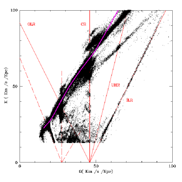
Figure 4: Frequency map for $D_{hs}$. Horizontal axis shows angular frequencies $(\Omega)$ and vertical axis shows radial frequencies $(\kappa)$. Each point represents the average frequencies of a particle over 1 Gyr. Clustering of points along straight lines with certain slopes indicates the presence of resonances. The lines are computed using the resonant condition (eq. 2). $\Omega_{B}$ is computed as the average pattern speed in this period of time. The main resonances are labeled. In addition, the dash lines correspond the CR, ILR and OLR of another non-axisymmetric pattern with a different pattern speed. The grey curve (magenta in the color version) is the result of the epicycle approximation which breaks inside the corotation radius, where the orbits are very elongated

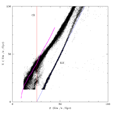
Figure 5: Frequency map for $K_{hb}$ (massive bar) for a period of 0.5 Gyr. As Fig. 4, lines indicate the main resonances and the grey curve (magenta in the color version) represents the epicycle approximation. The resonant structure shows a strong clustering of points along the ILR line. This is an indication of a large number of particles trapped near ILR orbits.

4.1 Detection of the main resonances

Once the orbital frequencies are measured in our three models, their main resonances become evident using frequency maps. They are commonly used to study resonances between planetary orbits in the Solar system (Laskar, 1990) and in orbital studies of elliptical galaxies (Holley-Bockelmann et al., 2001). In our case, a frequency map displays angular frequencies along the horizontal axis and radial frequencies in the vertical axis. This is a clear way to display the resonant structure of a model in the space of its orbital frequencies. Each point in this space represents the mean orbital frequencies of an individual particle over a fixed period of time. In a frequency map, all the orbits near a particular resonance lie along a line defined by the resonant condition (Eq. 2). $\Omega_{B}$ is computed as the average pattern speed in this period of time (Colín, Valenzuela & Klypin, 2006). Any set of integers defines a line in the frequency map. As a result, points along a given resonant line correspond to particles close to the resonance by definition.

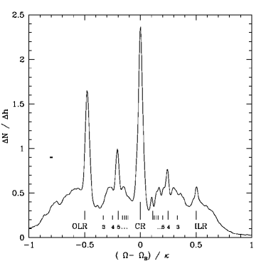
Figure 6: Distribution of the ratio $(\Omega-\Omega_{B})/\kappa$ for $D_{hs}$ for a period of 1 Gyr. The vertical axis shows the fraction of particles per unit of bin in the frequency ratio. Vertical lines represent low order resonances ($\pm 1$:m) and CR. The peaks show a strong indication of trapping resonances. The error-bar at the upper-left corner is the $1\sigma$ error using Poisson noise.

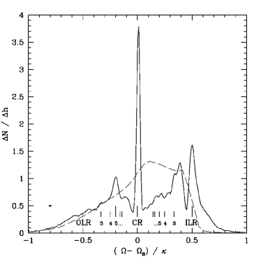
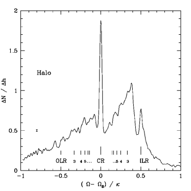
Figure 7: Distribution of the ratio $(\Omega-\Omega_{B})/\kappa$ for $K_{hb}$ for a period of 2 Gyr. The vertical axis shows the fraction of particles per unit bin in the frequency ratio. The error-bar on the left is the $1\sigma$ error using Poisson noise. Strong peaks at CR and ILR are clearly present. The dash line shows the distribution for a period of 0.5 Gyr before the formation of the bar. No peaks are found before the formation of the bar. The formation of these resonant peaks is linked to the capture of particles near resonant orbits.

Figure 8: Distribution of the ratio $(\Omega-\Omega_{B})/\kappa$ for particles in the halo chosen to stay close to the disk of $K_{hb}$. The lines shows resonances as Fig. 6 and 7. The CR and ILR are clearly present in the halo. The error-bar is the $1\sigma$ error using Poisson noise.

Fig. 4 shows the frequency map of the model $D_{hs}$ for 1 Gyr. We can clearly see concentration of particles near resonances. In particular, a narrow line of points is clearly visible along the ILR. This resonance covers a big range of angular and radial frequencies. The concentration of orbits near the CR is also especially strong. These particles are forced by the bar to rotate with the bar pattern speed. Other resonances are also visible. For example, the ultra-harmonic (-1:4) resonance (UHR) can be seen as a small cloud of points which intersects the line corresponding to the UHR. The OLR is very prominent. It intersects a line of constant angular frequency, $\Omega=27$ Km s^-1 Kpc^-1. This may be the CR of another non-axisymmetric pattern. This is supported by the fact that both OLR and ILR are also present for this second pattern. The OLR line is specially well populated. As a result, the model $D_{hs}$ may exhibit an overlap of resonances corresponding to two different non-axisymmetric features.

As another example, Fig. 5 shows the frequency map for the model $K_{hb}$ for a period of 0.5 Gyr. This model has a more massive bar which also rotates slower than in the model $D_{hs}$ discussed before. As a result, the resonant structure appears more compressed in this model. Its points extend over a smaller fraction of the frequency space. In addition, the corotation radius is larger. So, resonances beyond corotation, $\Omega<\Omega_{B}$, extend over the outer disk and they have less available material to capture. Therefore, OLR is not even present in this model. On the other hand, ILR is much stronger. It has more points clustered along the ILR line. This is the effect of a massive bar. The clustering of points near resonant lines in the frequency maps is a signature of trapped particles near resonant orbits.

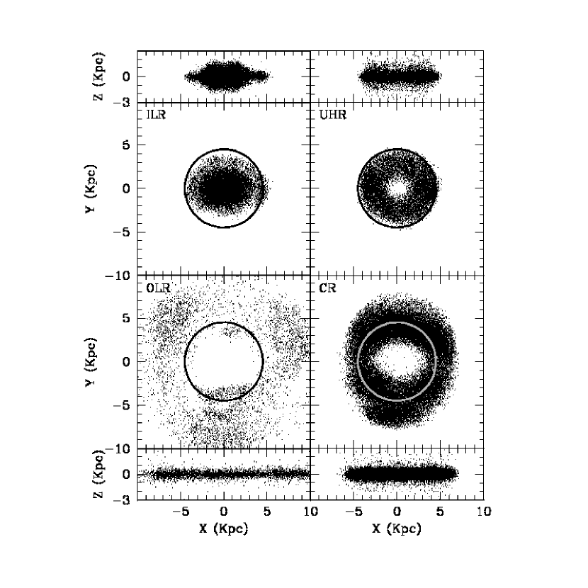
Figure 9: Spatial distributions of the particles at different resonances in $D_{hs}$. Each plot is labeled with the corresponding resonance. All resonances form rings except the ILR. This resonance is not localized at a given radius. A circle marks the corotation radius.

However, the majority of the points lies on a region spread diagonally across the frequency map. This feature is formed by particles at resonance, as well as particles out of resonance. It can be approximated by the epicycle approximation up to CR. We use the rotation curve of each model to estimate the epicycle frequencies. This approximation deviates from the dynamical frequencies inside the corotation radius. Orbits inside the corotation radius are elongated and their frequencies are higher than the expected values of nearly circular orbits. This is the region dominated by non-circular motions.

It is difficult to identify other resonances which lie on the crowded areas of a frequency map. As a result, we use the distribution of the ratio $(\Omega-\Omega_{B})/\kappa$ (Athanassoula, 2002) to detect the resonances of low order in l $(\pm 1:m)$. Each of these resonances has a unique value of this ratio. Fig. 6 shows the histogram of $(\Omega-\Omega_{B})/\kappa$ for the model $D_{hs}$ for a period of 1 Gyr. The distribution has peaks at the values of different resonances. We found 5 of them: OLR, (1:5), CR, (-1:4) and ILR. Fig. 8 shows the distribution of $(\Omega-\Omega_{B})/\kappa$ in $K_{hb}$ for a period of 2 Gyr. As we expected from the frequency map, the peak corresponding to the ILR is stronger than in $D_{hs}$. This is a common feature of systems with large bars.

In these histograms, there is an underlying distribution of particles which do not contribute to any resonant peak. They do not participate in any resonant motion with the bar. Thus, this background of particles should be present even before the formation of the bar. We performed a frequency analysis of the model $K_{hb}$ during the first 0.5 Gyr, before the bar formation. The distribution is shown in Fig. 8 as a dash curve. There are no significant peaks because there is no bar which captures particles near resonant orbits at this early stage of the simulation. As the simulation evolves, the bar forms and the distribution of $(\Omega-\Omega_{B})/\kappa$ changes dramatically. The tail of high frequencies and high values of $(\Omega-\Omega_{B})/\kappa$ grows. This is produced by particles that are sinking into the centre. However, the most dramatic change is the formation of the resonant peaks. Some particles are captured by the bar near some specific resonant orbits. This produces a clustering of particles near specific dynamical frequencies and the formation of the resonant peaks in the distribution of $(\Omega-\Omega_{B})/\kappa$. This clustering makes that the surrounding areas outside resonances are depopulated. This is reflected in gaps in the distribution of $(\Omega-\Omega_{B})/\kappa$ at both sides of a resonance. These gaps are very clear for CR and ILR of $K_{hb}$ but they are also visible for the (-1:5) and (1:4) resonances of $D_{hs}$.

We apply the same technique to find resonances in the halo. We select particles with a height from the plane lower than 3 Kpc. So, the particles are close to the disk. We also reject retrograde orbits. Fig. 8 shows the distribution of $(\Omega-\Omega_{B})/\kappa$ for the halo of $K_{hb}$ for a period of 2 Gyr. The pattern of resonances in the halo is very similar than the resonances in the disk. In particular, CR and ILR are clearly present.

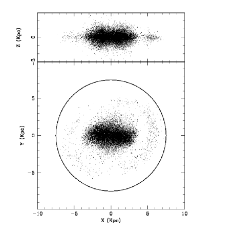
Figure 10: Spatial distribution of the particles at ILR in $K_{hb}$. The bottom panel shows a face-on view. The distribution resembles the bar. ILR particles can pass very close to the centre and span a wide range of radii. A circle marks the corotation radius. the top panel shows the vertical distribution. This edge-on view has a clear rectangular shape.

4.2 Spatial distribution of particles at resonances

We have seen the clustering of particles near resonances in the space of dynamical frequencies. But, what is their distribution in the coordinate space? Are they localized around a specific radius or are they spread over a broad region of the system? Fig. 9 shows the spatial distribution of the particles at the main resonances in $D_{hs}$. These are the disk particles which form the main peaks in the Fig. 6. They are confined into broad areas. Thus, particles near resonances populate a broad region of space. For example, particles trapped at CR stay at a broad ring around the corotation radius. However, the distribution is not uniform along the ring. There are fewer particles near the ends of the bar and more particles at both sides of the bar. This asymmetry is related to the position of the Lagrange points of the system, as we will see in §5. Other rings are also formed at UHR and OLR.

However, particles at ILR do not form a ring. The ILR is not localized around a given radius. Fig. 10 shows the particles near ILR for the model $K_{hb}$. They are concentrated in an elongated structure that resembles the bar. Particles at ILR can pass very close to the centre and they have very elongated orbits. As a result, they span a wide range of radii. This result implies that ILR extends over a broad range of energies. This fact was outlined in different papers. Athanassoula (2003) pointed the fact that the ILR resonant orbits are in fact the members of the x1 family of closed orbits. Athanassoula (1992) studied the energy range in which these resonant orbits are stable so they are able to capture orbits around them. They found that ILR orbits are stable over a significant range of values of the Jacobi energy. Weinberg & Katz (2007a) also found that ILR orbits extend up to very small radii.

In general, the vertical distribution near these resonances is very flat. This is expected because we are focused on planar resonances, so we do not expect resonant motions in the vertical direction. However, ILR is a clear exception. Its edge-on view has a clear rectangular shape (Fig. 10). This distribution again resembles the bar. Edge-on views of N-body bars show the same rectangular shape (Athanassoula & Misiriotis, 2002). A frequency analysis of motions in the vertical direction shows some particles trapped in the vertical ILR with the same values of their radial and vertical frequencies. The trajectories of these particles have their radial and vertical oscillations coupled.

5 Corotation capture

In previous sections, we saw that resonances can capture particles with specific frequency ratios. Now, we are going to focus on the details of this capture mechanism and we are going to describe what happens with the particles after being trapped near a resonance. We take CR, $\Omega=\Omega_{B}$, as an example, because it is easy to visualize. We use the model C of Valenzuela & Klypin (2003) to study the particles near CR. Particles which stay near CR during a period of 1 Gyr centred at 3.5 Gyr are selected. Fig. 11 and 12 show their spatial distribution and their density profiles at different moments. At 0.1 Gyr, just before bar formation, the particles are spread in an axisymmetric and extended distribution around the centre. This distribution is strongly affected by the formation of the bar. They gain angular momentum and evolve in a ring at the corotation radius. As a result, these particles evolve when they are being trapped at CR during the formation of the bar. After that, the distribution is stable for more than 4 Gyr or 20 bar rotations. As we discussed in $4.2$, the ring is not uniform. It shows a stronger concentration of particles in two broad areas $90^{\circ}$ away from the major axis of the bar. In addition, the surface density profile of these particles shows a stationary peak close to the corotation radius (Fig. 12). These particles are still trapped near CR several Gyr after the formation of the bar. Therefore, CR prevents a secular evolution in the trajectories of the particles trapped around it.

We can now study in detail how CR prevents the secular evolution of trapped particles in an almost stationary model, in which $\Omega_{B}$ is almost constant. We start with the spatial distribution of the change in angular momentum of particles in the disk. We compute the change of angular momentum of each particle between two different moments. That change contributes to the average angular momentum change at the position of the particle in an intermediate moment. The result is a field of angular momentum change. If these two moments are very close, that field is a good approximation of the instantaneous change of angular momentum in the disk. In other words, we are measuring the torque field produced by the bar and the spiral arms (Fig. 14). This torque has a similar shape of a torque from an elongated structure in rotation. It shows a $180^{\circ}$ symmetry. The bar is rotating in anti-clockwise direction. So, the particles which are close to the bar and moving ahead of the bar, are being pushed backwards by the bar. So, they loose angular momentum (black areas in Fig. 14). At the same time, particles which are moving behind the bar, are being pushed forwards. So, they gain angular momentum (dark grey areas in Fig. 14).

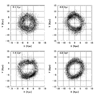
Figure 11: Spatial distribution of the particles selected for being near CR at 3.5 Gyr at 4 different moments. The particles are taken from the model C. At 0.1 Gyr, the bar is still not formed. After, bar formation, the distribution of these particles is stationary for more than 4 Gyr. Particles trapped near CR stay there for a long time. The circle represents the corotation radius.

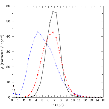
Figure 12: Evolution of the surface density profile of particles selected for being near CR at 3.5 Gyr for model C. The full curve corresponds to the distribution of the particles at 3.5 Gyr. The dotted curve shows the same particles at 0.1 Gyr, before the bar formation. The dashed line is for 4.5 Gyr, 1 Gyr after the moment in which the particles are selected for being at CR. As the bar forms, some particles get trapped near corotation radius. After that, the profile shows a peak centered at the corotation radius. The distribution shows little evolution for 4 Gyr.

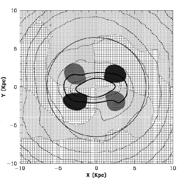
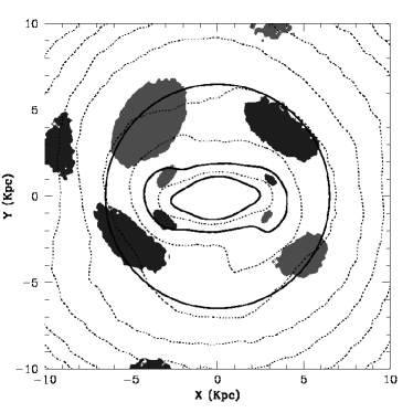
Figure 13: Spatial distribution of the instantaneous angular momentum change measured in a short interval of 28 Myr in model C. See electronic version of a color version of this plot. The two black leaves (dark blue) are areas with a strong negative torque. The two dark grey leaves (dark red) have a strong positive torque. Finally, the broad areas filled with squares (light blue) have a small negative torque, while the areas colored with a light grey ( light red) have a small positive torque. The bar is rotating in anti-clockwise direction. The particles which are close to the bar and moving ahead of the bar, loose angular momentum (black/blue areas). At the same time, particles which are moving behind the bar, gain angular momentum (dark grey/red areas).

Figure 14: Distribution of the peaks in the change in angular momentum in the disk for a longer period of time (150 Myr). The grey (red) areas show the position of the particles with the maximum increment in their angular momentum. The black (blue) areas show the position of the particles with the maximum decrement of angular momentum. Those areas lie mainly along the corotation radius (black circle)

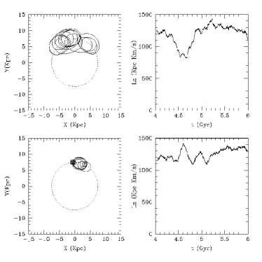
Figure 15: Example of two trajectories of particles near CR for 2 Gyr in the model $K_{hb}$. They are selected for being near CR between 4 Gyr and 4.5 Gyr. The left panels show their trajectories in the reference frame which rotates with the bar. The bar is always along the horizontal axis. The dotted circle is at the corotation radius. The example at the top is a trajectory in libration around an stable Lagrange point The trajectory at the bottom is even closer to this point. The right panels show the angular momentum of both trajectories over 2 Gyr. The angular momentum oscillates, but there is no overall change of angular momentum. These trajectories do not evolve. As a result, CR prevents the evolution for orbits trapped around it.

However, small changes in angular momentum over short periods of time can accumulate over a longer period. This can produce a much stronger change in angular momentum over a long period of time. Fig. 14 shows only the areas with the largest variations in angular momentum over a much longer interval of time than in Fig. 14. The selected interval is nearly one period of the bar, 150 Myr. The choice of different intervals produces similar results. The largest change of angular momentum lays mainly near the corotation radius and away from the major and minor axes of the bar. The two areas of positive change of angular momentum do not cover the same area. One is bigger than the other. However, this asymmetry is not permanent. It oscillates slowly with time. As a result, the net effect of this asymmetry is averaged out. Other peaks are also found inside the bar, a region dominated by ILR orbits. Finally, other peaks beyond the corotation radius could be attributed to the OLR.

Near the corotation radius, particles which are moving behind the bar for a significant interval of time accumulate small increments of angular momentum over that interval. The net effect is a significant increase in their angular momentum. The opposite is true for particles which stay ahead of the bar for a long period of time. They loose a significant amount of angular momentum. The main question is now how this change in angular momentum affects the evolution of these particles. The naïve idea is that a particle that increase its angular momentum evolves strongly. However, a particle initially in one of the areas of maximum positive change in angular momentum near CR (grey/red areas in Fig. 14) gains angular momentum and moves outwards. As a result, the particle rotates slower than the bar, $\Omega<\Omega_{B}$. It lags the bar and starts to move to the area of negative angular momentum change (black/blue areas in Fig. 14). In that area, the particle looses the angular momentum gained previously and moves inwards. As a result, it starts to rotate faster than the bar, $\Omega>\Omega_{B}$, and to move towards the area of positive change of angular momentum. In that area, the particle gains angular momentum and the cycle starts again. As a result, the changes in angular momentum are compensated along the trajectory of each particle near CR. These oscillations of angular momentum produces no net torque over a long period of time. CR actually prevents the evolution of the particles trapped near the corotation radius.

Fig. 15 provides two examples which illustrate this previous idea. They are taken from the model $K_{hb}$. The particles are selected to be near CR between 4 and 4.5 Gyr. Then, we plot their trajectories for the next 2 Gyr. We select the non-inertial frame which rotates with the bar. In that frame, the bar is always along the horizontal axis and a particle exactly at CR is not moving in this frame. The top panels of Fig. 15 show a particle which slowly oscillates once along a section of the corotation ring during 2 Gyr. The particle moves between the areas in which the change of angular momentum is positive and negative. As a result, the changes in its angular momentum cancel each other. The net result of this oscillation is an almost no change in the angular momentum. The particle is trapped in an orbit of libration for several Gyr and many orbits.

The bottom panels of Fig. 15 show an orbit closer to CR. It also librates at the corotation radius but the amplitude of the oscillations are much smaller than in the previous case. Actually, during the last Gyr of the simulation, the particle spends several orbits around a single point in the rotating frame. The angular momentum during this time is almost constant. So, the net transfer of angular momentum near that point is minimum. In other examples, the orbits librate in a similar way but around another point on the other side of the corotation ring.

This trapping mechanism near CR is actually well known in galactic and celestial mechanics. The situation is equivalent to the motions of arbitrary amplitude around the stable Lagrange points of a stationary non-axisymmetric system. The equations of motion can be reduced to the equations of a pendulum (Binney & Tremaine, 1987, Chapter 3, eqs. (3-123)-(3-129) ). Particles trapped near CR librate slowly around one of the stable Lagrange points. A particle exactly at this point is exactly at CR. A close example of such resonant orbit is shown in the bottom panels of Fig. 15. This orbit moves along the corotation radius with the same angular velocity of the bar rotation. CR keeps particles in libration orbits for a long time and for many periods. While particles are trapped, their orbits do not evolve. As a result, CR prevents the evolution of the particles trapped around it and minimize their angular momentum transfer.

6 Comparison with an analytical model

As we saw in the previous section, CR captures particles around two stable Lagrange points. The stability around these points is mainly determined by the topology of the gravitational potential around them. Therefore, we can approximate this potential with a simple analytical model which captures the main features of a strongly barred system. Such a model can be used to clarify the results of N-body simulations. The analytical potential consists of a Miyamoto disk, a NFW halo and a homogeneous prolate ellipsoid. The ellipsoid rotates with a given pattern speed $\Omega_{B}.$ The corresponding expressions are described in appendix A and the parameters of the model are given in Table 3. It reproduces a strongly barred galaxy. Its circular velocity profile is shown in Fig. 16. Using this background potential, we can compute the trajectories of a set of particles and follow their resonant interactions with the bar. This analytical model can catch some fundamental aspects of resonances, like trapped orbits near resonances. At the same time, this simple model does not have the inherent complexity of a self-consistent N-body simulation. As a result, it is easy to interpret. Then, this interpretation can be used to understand better the resonant phenomena in more complex and realistic cases, like in N-body models.

Table 3: Set of parameters for the analytical model.

Miyamoto disk:
Disk Mass ($10^{10}{\rm M}_{{}_{\mathord{\odot}}\;}$)	5
A (kpc)	4
B (kpc)	1
NFW halo:
$r_{s}$ (Kpc)	28.7
$\rho_{0}$ ($10^{6}{\rm M}_{{}_{\mathord{\odot}}\;}$ Kpc${}^{-}3$ )	3.12
Prolate ellipsoid:
Bar mass ($10^{10}{\rm M}_{{}_{\mathord{\odot}}\;}$)	1
Semimajor axis (Kpc)	4
Semiminor axis (Kpc)	1
Pattern speed (km s-1 Kpc-1)	36

Figure 16: Circular velocity profile of the analytical model of a barred galaxy. The model corresponds to a typical high surface brightness barred galaxy with a maximum circular velocity close to 190 km s^-1.

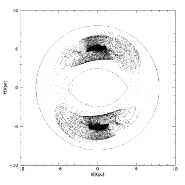
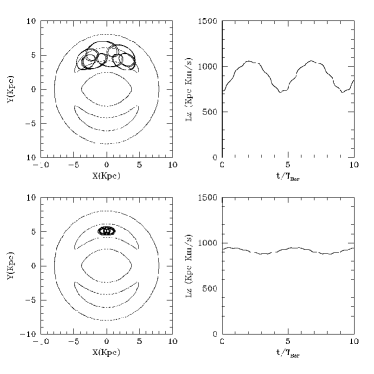
Figure 17: Spatial distribution of the particles trapped at CR after 100 bar rotations (17 Gyr) The distribution fills two lobes around the stable Lagrange points. It resembles the distribution of particles trapped near CR in the N-body models (Fig. 9 and 11). The background contours are contours of equal effective potential.

Figure 18: Two examples of trajectories trapped near CR, as in Fig. 15. The trajectories librate around the stable Lagrange point and their angular momentum oscillate with no net change of angular momentum after approximately 5 bar periods.

Fig. 18 shows particles trapped near CR at two stable Lagrange points. The initial configuration is a set of $32^{3}$ particles distributed uniformly inside two small spheres of 0.1 Kpc in radius. Each one is centered at each stable Lagrange point. The distribution of velocities is initially centered on the circular velocity at the corotation radius. The dispersion is 25 per cent of that velocity. After 100 bar rotations, almost all particles fill two banana-shape areas at both sides of the bar. They are still trapped around the stable Lagrange points. They cover a broad area along the corotation radius. This supports the results discussed in $\S 5$ for a self-consistent N-body experiment. The distribution of the particles near CR in Fig. 9 and 11 resembles the distribution of the particles trapped around the two stable Lagrange points in Fig. 18. The region of trapped particles is not an infinitesimal volume around the stable points. It extends over a broad volume both in spatial and phase space. The distribution of the energies of these particles cover a range which is 10 per cent of the energy at the Lagrange point. CR covers a significant volume in phase space, although the only particle formally at resonance is the one which moves with one of the stable points.

In general, these trapped particles move in libration orbits around the Lagrange points. They are trapped for a cosmologically significant period of time. Fig. 18 shows two examples of libration orbits and the change of their angular momentum. These examples can be compared with the examples taken from the N-body model and discussed in §5. The first example has large amplitude of libration. As a result, the angular momentum oscillates significantly. However, the angular momentum oscillates and the net change is canceled in a libration period. As a result, the net angular momentum transfer over many orbits is zero. The bottom panels of Fig. 18 show another example. Its amplitude of libration is much smaller than in the first example. The oscillations in the angular momentum are also much smaller. This example is similar to the second example of §5. The particle is closer to CR and remains in a stable orbit which minimizes the transfer of angular momentum. This supports the interpretation that resonances prevent the orbital evolution of trapped particles.

Similar conclusions can be obtained for other resonances. In the case of the ILR, the resonant orbits are closed orbits elongated along the bar. The top panels of Fig. 19 show an example of a ILR orbit. The angular momentum oscillates significantly but the net change of angular momentum averaged over one orbit is zero. As we pointed in $\S 4.2$, the ILR orbits are known as the $x1$ family. They are the backbone of the orbits which support the bar (Skokøs et al., 2002; Athanassoula, 1992). These resonant orbits capture particles around them in a similar way corotation does. The bottom panels of Fig. 19 show one example of a trajectory trapped around the ILR orbit. The trajectory librates around the closed orbit. The angular momentum is modulated by this libration but again the net average change over many periods is zero. The main difference between CR and ILR is that ILR orbits are a set of orbits instead of two Lagrange points. The result is that the ILR resonance covers a larger volume in phase space which cover the bar, as we saw in the distribution of ILR particles in Fig. 10. The trajectories in Fig. 19 are stable forever. We tracked them for more than 100 bar rotations and there is no indication of evolution in their trajectories. As we saw before, particles trapped at resonance do not evolve. For the ILR, particles are trapped by a set of $x1$ orbits and forced to move within the bar as the bar rotates.

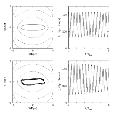
Figure 19: Two examples of trajectories as in Fig. 15 but for the ILR. The top panels show an example of a ILR orbit. The angular momentum oscillates but average change of angular momentum is zero. The bottom panels show one example of a trajectory trapped around the ILR orbit. The trajectory librates around the closed orbit. The angular momentum is modulated by this libration but again the net average change over many periods is zero.

However, what happens with the particles trapped at resonance when the bar evolves? In this case, the resonant structure also evolves. The volume in the phase-space which satisfies a particular resonant condition drifts through the phase-space. Does the trajectory initially trapped at a resonance follow it or is scattered off resonance? In order to address this issue, we follow the same ILR trajectories when the bar slows its rotation. The top panels of Fig. 20 show the imposed bar pattern speed. It remains constant for 30 initial bar rotations (5 Gyr), then it decreases linearly for other 30 initial bar rotations and finally remains constant for 40 initial bar rotations. At the end, the bar pattern speed decreases to 40 per cent of its original value over 5 Gyr. From each trajectory, we extract the specific angular momentum averaged over time for an orbit in the rotating frame and its radial and angular frequencies over the orbit. The radial frequency is computed as $\kappa=2\pi/T_{p}$, where $T_{p}$ is the period of the radial oscillations, defined as the time between apocenters. At the same time, the angular frequency is defined as $\Omega=\Delta\Phi/T_{p}$, where $\Delta\Phi$ is the angle swept by the trajectory between apocenters in the inertial frame. Using these frequencies and the pattern speed of the bar, we can check the resonant condition for ILR (Eq. 2).

The left side of Fig. 20 shows the orbit which is initially trapped exactly at ILR. Before any evolution, the averaged angular momentum remains constant and the resonant condition is fulfilled. During the slowdown of the bar, the angular momentum of the trajectory decreases at almost the same rate of the change in the pattern speed. The trapped particle follows the slowdown of the bar. More important is the fact that the trajectory remains close to the resonance although the system evolves. The particle is trapped at resonance and oscillates around the resonant orbit as the system evolves as a whole. This tracking of a resonance is true even for trajectories further from the exact resonant orbit but still trapped around it. The right side of Fig. 20 shows an example. The oscillations around the resonant condition are larger than in the previous case, but the trajectory is not scattered off resonance when the system evolves. The same results can be found for bigger rates of change in the pattern speed. Only when the pattern speed decreases to one half of its original value in less than one bar period, the oscillations around the resonant condition become wider.

Figure 20: Left and right panels show two different examples of particles near ILR when the bar slows its rotation during 30 bar rotations between 30 and 60 bar rotations. Top panels show the evolution of the bar pattern speed. Middle panels show the evolution of the angular momentum averaged over a single orbit. Bottom panels show the ILR condition (eq. 2) scaled by $\Omega_{B}$. During the slowdown of the bar, the trajectory exactly at ILR(left) and the trajectory trapped near ILR(right) remain near resonance. They track the resonance and follow the bar evolution.

7 Discussion

Resonances play an important role in barred galaxies. Stable resonant orbits can capture disk and halo material in near-resonant orbits. The bar itself is a manifestation of this resonant capture. The $x1$ family of closed orbits are ILR resonant orbits that capture particles in elongated orbits along the bar major axis (Athanassoula, 2003). These orbits support the orbital structure of the bar (Skokøs et al., 2002; Athanassoula, 1992).

Resonances prevent the dynamical evolution of the material trapped near resonant orbits. This material does not experience a net change of angular momentum although the angular momentum oscillates strongly over an orbital period (Fig. 19). A particle exactly at resonance with the bar has no evolution in its trajectory. The change in angular momentum over an orbital period is zero. The particle exactly at resonance stay at a resonant closed orbit forever. As a result, resonances tend to minimize the exchange of angular momentum between trapped material and the bar.

Therefore, the mere presence of resonances in barred galaxies do not drive their secular evolution. Orbits trapped at resonance only evolve if the bar evolves as a whole (Fig. 20). In this case, resonances drift as the bar evolves. Particles anchored near resonant orbits track the resonances and consequently evolve. As a result, the evolution at resonances is linked to the evolution of the bar. For example, if the bar slows its rotation, the Lagrange points move outwards. As a result, CR moves outwards and trapped particles, which track the motion of CR, move also outwards. The result is that these particles near CR gain angular momentum and evolve. At the same time, ILR particles trapped by the bar loose angular momentum. This angular momentum is not lost because the particles are near a resonance. It is lost because there is a net torque, which produces a slowdown of the bar and of the trapped particles trapped near ILR.

This torque can be the result of the dynamical friction with the dark matter halo. Resonances in the halo can also play an important role in this interaction. ILR particles in the halo form an ellipsoidal structure in the inner halo. (Colín, Valenzuela & Klypin, 2006). This halo bar exerts a torque on the stellar bar that slows its rotation. This is an interaction between different structures trapped at ILR. As a result of this interaction, ILR particles in the stellar bar can loose angular momentum and ILR particles in the halo can gain it. This interpretation is consistent with the results on the angular momentum change near resonances in the case of the bar slowdown (Athanassoula, 2003). However, this mechanism of change of angular momentum at resonances is very different from the resonant transfer of angular momentum predicted in perturbation theory (Athanassoula, 2003; Lynden-Bell & Kalnajs, 1972).

The resonances found in Athanassoula (2003) are consistent with the resonances found in our models. However, the models in Athanassoula (2003) have a stronger ILR, CR was weaker and outer resonances like OLR were almost absent. These differences are due to differences in the corotation radius. Based on the initial rotation curve and the pattern speed of the model MQ2 of Athanassoula (2003), the corotation radius was roughly 20 Kpc, 5.7 times its disc scalelength. This is 5 times larger than the corotation radius in our model $D_{hs}$. Thus, the models in Athanassoula (2003) have most of the material of the disk within the corotation radius. This material can only be captured by inner resonances like ILR. That results in a strong ILR peak. On the other hand, little material lies at corotation radius and beyond. Therefore, CR, OLR and other outer resonances can trap only a few particles. This is why their peaks in the $(\Omega-\Omega_{B})/\kappa$ histogram of Athanassoula (2003) are much smaller than in our model $D_{hs}$.

Recently, Weinberg & Katz (2007a) discussed the dynamics of the interaction between a bar and a dark matter halo and described the requisites needed to follow this resonant interaction accurately. The first criterion stated that a N-body model should have enough phase-space coverage at resonances. In order to ensure the correct resonant behavior, the phase space near resonances should be populated with enough particles. The phase-space volume near resonances is defined by the separatrix which divides trapped from non-trapped orbits in the phase space near a resonance. This volume covers the region of trapped orbits which librate around the stable resonant orbit. Weinberg & Katz (2007a) argue that 10 particles inside one tenth of that resonant region are enough to obtain the correct behavior at resonances. Our model $D_{hs}$ has around $1.5\times 10^{4}$ disk particles near ILR and $4.1\times 10^{4}$ near CR. These are trapped particles which stay in the libration region near resonances. As a result, resonances are well populated in our N-body models. This is because the region of trapped orbits is large (Fig. 6, 8, 8).

The second criterion deals with the artificial noise in the potential and the effects of two-body scattering. They can introduce an artificial diffusion of orbits. The characteristic diffusion length should be smaller than the resonance width, defined by the size of the region of trapped orbits. Otherwise, particles can artificially diffuse out of a resonance. We have seen that these regions near resonances are large. So, this second criterion is also achieved.

8 Summary and conclusions

We have detected dynamical resonances in N-body models of barred galaxies with evolving disks in live dark matter halos. The dominant resonances are the corotation resonance (CR) and the inner Lindblad resonance (ILR), although other low order resonances, like the outer Lindblad resonance (OLR) or the ultra-harmonic resonance (UHR) are also present (Fig. 6, 8, 8). Resonances in the halo are also found.

In general, resonances cover broad areas of the disk (Fig. 9). Particles at CR are distributed in a wide ring at the corotation radius. On the other hand, the epicycle frequencies are not equal to the natural frequencies of particles inside the corotation radius, where non-circular motions are important. This is specially true for the ILR. this resonance is not localized at a given radius. Particles at ILR are found mainly in elongated orbits inside the bar. Their distribution resembles the bar (Fig. 10)

In all three studied models, we find that resonances capture particles and force them to move in trajectories near stable resonant orbits. For example, the corotation resonance traps particles in libration orbits around the two stable Lagrange points of the system. As a result, the angular momentum oscillates with the period of the libration motion but the net change over many orbits is zero. Therefore, these trapped particles do not evolve. We conclude that resonant trapping tends to minimize the change of angular momentum of the particles trapped around them. However, the trapped particles can participate in the global evolution of the bar because they are locked at resonances. They are still trapped during the slowdown of the bar (Fig. 20). As a result, ILR particles can loose angular momentum during this slowdown. Particles trapped at resonances only evolve when the bar evolves as a whole.

Appendix A An analytical galactic potential

The 3D potential used in §6 consists of three components. First, A Miyamoto potential represents the disk:

$$\Phi_{D}(\mathbf{x})=-\frac{GM_{D}}{\sqrt{x^{2}+y^{2}+(A+\sqrt{B^{2}+z^{2}})^{2}}}$$ (13)

where $M_{D}$ is the mass of the disk, A and B are the horizontal and vertical scalelengths. The dark matter halo is modeled using a NFW halo:

$$\Phi_{H}(\mathbf{x})=-4\pi G\rho_{s}r_{s}^{2}\frac{\ln(1+r/r_{s})}{r/r_{s}},\ r=\sqrt{x^{2}+y^{2}+z^{2}}$$ (14)

Finally, the contribution of the bar is modeled as a prolate homogeneous ellipsoid. The potential of a point inside the ellipsoid is given by

$$\Phi_{B}(\mathbf{x})=-\pi G\rho\left(I(\mathbf{a})a_{1}^{2}-\sum A_{i}(\mathbf{a})x_{i}^{2}\right)$$ (15)

where $x_{i}=\{x,y,z\},i=1,3$. $a_{1}$ is the semimajor axis of the bar and $a_{2}=a_{3}$ is the semiminor axis. $I(\mathbf{a})$ and $A_{i}(\mathbf{a}),i=1,3$ are defined by the relations:

$$I(\mathbf{a})=\frac{1}{e}\ln\frac{1+e}{1-e}$$ (16)

$$e=\sqrt{1-\frac{a_{1}^{2}}{a_{3}^{2}}}$$ (17)

$$A_{1}(\mathbf{a})=\frac{1-e^{2}}{e^{2}}\left[\frac{1}{1-e^{2}}-\frac{1}{2e}\ln\frac{1+e}{1-e}\right]$$ (18)

$$A_{2}(\mathbf{a})=A_{1}(\mathbf{a})$$ (19)

$$A_{3}(\mathbf{a})=2\frac{1-e^{2}}{e^{2}}\left[\frac{1}{2e}\ln\frac{1+e}{1-e}-1\right]$$ (20)

Similarly, the potential of a point outside the ellipsoid is given by:

$$\Phi_{B}(\mathbf{x})=-\pi G\rho\frac{a_{1}a_{2}a_{3}}{\acute{a}_{1}\acute{a}_{2}\acute{a}_{3}}\left(I(\mathbf{\acute{a}})\acute{a}_{1}^{2}-\sum A_{i}(\mathbf{\acute{a}})x_{i}^{2}\right)$$ (21)

where

$$\acute{a}_{i}^{2}=a_{i}^{2}+\lambda(\mathbf{x}):\sum\frac{x_{i}}{\acute{a}_{i}^{2}}=1.$$ (22)

References

- Arnold & Avez (1968) Arnold V. I., Avez A., 1968, Ergodic problems of classical Mechanics, W.A. Benjamin, Inc.
- Athanassoula (1992) Athanassoula E., 1992, MNRAS, 259, 328
- Athanassoula (2002) Athanassoula E., 2002, ApJ, 569, L83
- Athanassoula & Misiriotis (2002) Athanassoula E., Misiriotis A., 2002, MNRAS, 330, 35
- Athanassoula (2003) Athanassoula E., 2003, MNRAS, 341, 1179
- Binney & Tremaine (1987) Binney J., Tremaine S., 1987, Galactic Dynamics. Princeton Univ. Press, Princeton, NJ
- Byrd, Freeman & Buta (2006) Byrd G., Freeman T., Buta R., 2006, AJ, 131, 1377
- Chirikov (1960) Chirikov B. V., 1960, Journal of Nuclear Energy, 1, 253
- Colín et al. (2000) Colín P., Klypin A., Kravtsov A., 2000, ApJ, 539, 561
- Colín, Valenzuela & Klypin (2006) Colín P., Valenzuela O., Klypin A., 2006 ApJ, 644, 687
- Contopoulos & Grosbøl (1989) Contopoulos G., Grosbøl P., 1989, A&AR, 1, 261
- Eskridge et al. (2000) Eskridge P. B., et al. 2000, AJ, 119, 536
- Hernquist (1993) Hernquist L., 1993, ApJS, 86, 389
- Holley-Bockelmann et al. (2001) Holley-Bockelmann K., Mihos J. C., Sigurdsson S., Hernquist L., 2001, ApJ, 549, 862
- Holley-Bockelmann et al. (2005) Holley-Bockelmann K., Weinberg M., Katz N., 2005, MNRAS, 363, 991
- Klypin et al. (2002) Klypin A., Zhao H., Somerville R., 2002, ApJ, 573, 597
- Kravtsov et al. (1997) Kravtsov A., Klypin A. , Khokhlov A. M., 1997, ApJS, 111, 73
- Kravtsov (1999) Kravtsov A., 1999, Ph.D. thesis, New Mexico State Univ.
- Laskar (1990) Laskar J., 1990, Icarus, 88, 266
- Lichtenberg & Lieberman (1983) Lichtenberg A. J., Lieberman M. A., 1983, Regular and Stochastic Motion. Springer-Verlag, New York
- Lynden-Bell & Kalnajs (1972) Lynden-Bell D., Kalnajs A. J., 1972, MNRAS, 157, 1
- Martinez-Valpuesta et al. (2006) Martinez-Valpuesta I., Shlosman I., Heller C., 2006, ApJ, 637, 214
- Murray & Dermott (1999) Murray C. D., Dermott, 1999, Solar system Dynamics, Cambridge University Press Princeton, NJ
- Navarro et al. (1997) Navarro J. F., Frenk C. S., White S. D. M., 1997, ApJ, 490, 493
- Skokøs et al. (2002) Skokøs Ch., Patsis P.A., Athanassoula E., 2002, MNRAS, 333, 847
- Tremaine & Weinberg (1984) Tremaine S., Weinberg M.D., 1984, MNRAS, 209, 729
- Valenzuela & Klypin (2003) Valenzuela O., Klypin A., 2003, MNRAS, 345, 406
- Voglis, Tsoutsis & Efthymiopoulos (2006) Voglis N., Tsoutsis P., Efthymiopoulos C., 2006, MNRAS, 373, 280
- Weinberg (2004) Weinberg, M. D., 2004, preprint (astro-ph/0404169)
- Weinberg & Katz (2007a) Weinberg M. D., Katz N., 2007a, MNRAS, 1499
- Weinberg & Katz (2007b) Weinberg M. D., Katz N., 2007b, MNRAS, 1500