Traveling waves in magnetized Taylor-Couette flow

Abstract

We investigate numerically a traveling wave pattern observed in experimental magnetized Taylor-Couette flow at low magnetic Reynolds number. By accurately modeling viscous and magnetic boundaries in all directions, we reproduce the experimentally measured wave patterns and their amplitudes. Contrary to previous claims, the waves are shown to be transiently amplified disturbances launched by viscous boundary layers rather than globally unstable magnetorotational modes.

I Introduction

The luminosity of most astrophysical accretion disks probably depends upon the magnetorotational instability (MRI)Balbus and Hawley (1998), which has inspired searches for MRI in Taylor-Couette flow. Standard MRI modes will not grow unless both the rotation period and the Alfvén crossing time are shorter than the timescale for magnetic diffusion. This requires that both the magnetic Reynolds number $Re_{\rm m}\equiv\Omega_{1}r_{1}(r_{2}-r_{1})/\eta$ and the Lundquist number $S\equiv V_{Az}^{0}(r_{2}-r_{1})/\eta$ be $\gtrsim 1$, where $V_{Az}^{0}=B_{z}^{0}/\sqrt{4\pi\rho}$ is the Alfvén speed and $B_{z}^{0}$ is the background magnetic field parallel to the angular velocity $\boldsymbol{\Omega}=\Omega\boldsymbol{e}_{z}$. No laboratory study of standard MRI has been completed except for that of Sisan et al. (2004), whose experiment proceeded from a background state that was already hydrodynamically turbulent before the field was applied. Recent linear analyses of axially periodic or infinite magnetized Taylor-Couette flow has shown that MRI may grow at much reduced $Re_{\rm m}$ and $S$ in the presence of a combination of axial and current-free toroidal field Hollerbach and Rüdiger (2005); Rüdiger et al. (2005). We call such modes “helical” MRI (HMRI)

The PROMISE (Potsdam Rossendorf Magnetic Instability Experiment) group have claimed to observe HMRI experimentally Stefani et al. (2006); Rüdiger et al. (2006); Stefani et al. (2007). At magnetic and flow parameters where linear analysis predicts instability, persistent fluctuations were measured that appeared to form axially traveling waves, consistent with expectations for HMRI. Similar behavior has been seen in nonlinear numerical simulations that approximate the experimental conditions, including realistic viscous boundary conditions for the velocities, but simplified ones for the magnetic field: perfectly conducting cylinders, and pseudo-vacuum conditions at the endcaps, when present Stefani et al. (2007); Szklarski and Rüdiger (2006). Both axially periodic and finite cylinders showed unsteady flow, the former case being more regular. However, the nonlinear simulations in Stefani et al. (2007); Szklarski and Rüdiger (2006) used somewhat different values for the cylinder rotation rates and other parameters than those reported in Stefani et al. (2006).

Previously, however, we have raised doubts about both the experimental realizability of HMRI and its astrophysical relevanceLiu et al. (2006a). Finite cylinders with insulating endcaps were shown to reduce the growth rate and to stabilize highly resistive flows entirely, at least inviscid ones.

Here we report nonlinear simulations with the ZEUS-MP 2.0 code Hayes et al. (2006), which is a time-explicit, compressible, astrophysical ideal MHD parallel 3D code, to which we have added viscosity, resistivity (with subcycling to reduce the cost of the induction equation), and vacuum boundary conditions, for axisymmetric flows in cylindrical coordinates $(r,\varphi,z)$Liu et al. (2006b). The parameters of PROMISE as reported in or inferred from Stefani et al. (2006) are used: gallium density $\rho=6.35\,{\rm g\;cm^{-3}}$, magnetic diffusivity $\eta=2.43\times 10^{3}\,{\rm cm^{2}\;s^{-1}}$, magnetic Prandtl number $Pr_{\rm m}\equiv\nu/\eta=1.40\times 10^{-6}$; Reynolds number $Re\equiv\Omega_{1}r_{1}(r_{2}-r_{1})/\nu=1775$; axial current $I_{z}=6000\,{\rm A}$; toroidal-coil currents $I_{\varphi}=0,50,75,120\,{\rm A}$; and dimensions as in Fig. 1. For the first time, the finite conductivity and thickness of the copper vessel are allowed for ($\eta_{\rm Cu}=1.335\times 10^{2}\,{\rm cm^{2}s^{-1}}$), and this noticeably improves agreement with the measurements compared to previous linear calculations with radially perfectly conducting, axially periodic boundaries Stefani et al. (2006); Rüdiger et al. (2006). Please note the difference of the direction of $\Omega$, $B_{z}$ and $B_{\varphi}$ (components measured in a right handed coordinate system) between this paper, where they are all assumed to be positive, and the experimental setup presented in Stefani et al. (2006), where they are all negative (private communication). The direction of the traveling wave depends on the sign of the Poynting flux defined as $-r\Omega B_{\varphi}B_{z}/\mu_{0}$ Liu et al. (2006a). Thus the direction of the traveling wave reported here is opposite as reported in Stefani et al. (2006).

II Boundary Conditions

At the low frequencies relevant to PROMISE ($f\sim 0.01\,{\rm Hz}$), the skin depth of Copper $\delta_{w}=\sqrt{\eta_{\rm Cu}/\pi f\mu_{0}}\approx 19\,{\rm cm}$, which is much larger than the thickness of the copper vessel surrounding the gallium in the PROMISE experiment, $d_{w}\approx 1.0\,{\rm cm}$, so that the magnetic field diffuses rather easily into the boundary. On the other hand, if one considers axial currents, the gallium and the copper wall act as resistors in parallel; taking into account their conductivities and radial thickness, one finds that their resistances are comparable [$R_{I}:R_{II}:R_{III}=3:1:9$; see Fig. 1 for the subscripts]. Therefore, the currents carried by the copper walls could be important for the toroidal field, and a perfectly insulating boundary condition is also inappropriate.

Figure 1: Computational domain for simulations of PROMISE experiment. Region (I): Inner copper cylinder, angular velocity $\Omega_{1}$. (II): outer copper cylinder and bottom endcap, $\Omega_{2}$. (III): liquid gallium; (IV): vacuum. Thick dashed line: insulating upper endcap, $\Omega=0$. Dimensions: $r_{1}=4.0\,{\rm cm}$; $r_{2}=8.0\,{\rm cm}$; $h=40.0\,{\rm cm}$; $d_{wI}=1.0\,{\rm cm}$; $d_{wII}=1.5\,{\rm cm}$; $\Omega_{1}/2\pi=3.6\,{\rm rpm}$; $\Omega_{2}/2\pi=0.972\,{\rm rpm}$. The exact configuration of the toroidal coils being unavailable to us, six coils (black rectangles) with dimensions as shown were used, with $67$ turns in the two coils nearest the midplane and $72$ in the rest. Currents $I_{\varphi}$ were adjusted to reproduce the reported Stefani et al. (2006) Hartmann numbers $Ha\equiv B_{z}^{0}r_{1}/\sqrt{\rho\mu_{0}\eta\nu}$.

We have adapted a linear axisymmetric code developed by Goodman and Ji (2002); Liu et al. (2006a) to allow for a helical field. Vertical periodicity is assumed, to allow separation of variables, but the full viscous and resistive radial equations are solved using finite differences, and a variety of radial boundary conditions can be imposed. For perfectly conducting boundaries and $I_{\varphi}=75\,{\rm A}$, where Stefani et al. (2006) report persistent waves, our code indeed finds a complex growth rate: $s\approx 0.0057+0.057i\,{\rm s^{-1}}$. But for insulating boundaries, the same parameters yield stability.

This analysis points to the need for boundary conditions that accurately represent the influence of the copper vessels on the field. In the linear code just mentioned, we use the thin-wall approximation of Müller and Bühler (2000), which in effect treats the cylinders as insulating for the poloidal field but conducting for the toroidal field. The errors of this approximation increase with the ratio of wall thickness to gap width, which is not very small ($\approx 0.25$) in our case. Growth is predicted, but at a smaller rate than for perfectly conducting walls, $s\approx 0.0052+0.056\,i\leavevmode\nobreak\ \,{\rm s^{-1}}$. The insensitivity of the imaginary part to the magnetic boundaries supports the interpretation that these modes are hydrodynamic inertial oscillations weakly destabilized by the helical field Liu et al. (2006a).

In our nonlinear simulations, we include the copper walls (regions I and II) in the computational domain (Fig. 1), but not the external coils themselves, whose inductive effects are therefore neglected. Outside the walls (region IV) we match onto a vacuum field $\boldsymbol{B}_{\rm ext}=\boldsymbol{\nabla}\Phi$ vanishing at infinity. This is relatively straightforward in spherical geometry (used by many geodynamo experiments) because Laplace’s equation separates. Our case is more difficult, because while Laplace’s equation separates in cylindrical coordinates when the boundary is an infinite cylinder, it does not fully separate outside a finite cylinder. Therefore we use an integral formulation that does not assume separability. The idea, called von Hagenow’s method Lackner (1976), is to find a surface current on the boundary that is equivalent to the current density in the interior as the source for $\boldsymbol{B}_{\rm ext}$ via the free-space Green’s function. The surface current is obtained by first solving the Grad-Shafranov equation Grad and Rubin (1958); Shafranov (1966) in the interior with conducting boundary conditions, a problem that is separable in our case and is solved efficiently by combining FFTs along $z$ with tridiagonal matrix inversion along $r$.

III Results and Discussion

We start with purely hydrodynamic (unmagnetized) simulations. For $\mu\equiv\Omega_{2}/\Omega_{1}=0.27$, what we see is simply an Ekman flow driven by the top and bottom end plates. Due to the stronger pumping at the upper, stationary lid, the two Ekman cells are of unequal size. They are separated vertically by a narrow, intense radial outflow, hereafter the “jet”, lying at about $11\,{\rm cm}$ above the bottom endcap. As discussed in Kageyama et al. (2004), the jet is unsteady at $Re\gtrsim 10^{3}$; it flaps or wanders rapidly in the poloidal plane. This has been verified by the PROMISE group (private communication). The amplitude of the flapping is $\pm 0.4\,{\rm mm\;s^{-1}}$.

Figure 2: (color). Axial velocities $[\,{\rm mm\;s^{-1}}]$ versus time and depth sampled $1.5\,{\rm cm}$ from the outer cylinder, for the parameters of the PROMISE experiment Stefani et al. (2006) with toroidal currents $I_{\varphi}$ as marked. Note height increases upward from the bottom endcap. No-slip velocity boundary conditions are imposed at the rigidly rotating endcaps, but the steady part of the resulting Ekman circulation is suppressed in these plots by subtracting the time average at each height. The waves appear to be absorbed near the Ekman jet, at $z\approx 100\,{\rm mm}$.

     

Figure 3: (color). Panel (a): An extended version of the case $I_{\varphi}=75\,{\rm A}$ shown in Fig. 2 but without subtraction of the time average. The two Ekman cells are visible as the upflow (orange) at $z>100\,{\rm mm}$ and downflow (blue) at $z<100\,{\rm mm}$; these are the expected directions of flow near the outer cylinder. Panel (b): The same case again, except that after $t=360\,{\rm s}$, the no-slip boundary condition at both endcaps is changed to an ideal Couette profile, i.e. $\Omega(r)=a+br^{-2}$ with $a$ and $b$ chosen to make $\Omega$ continuous at both cylinders; this eliminates Ekman circulation. Thereafter, the wave seems to be absorbed near the bottom ($z\approx 0\,{\rm mm}$) rather than the jet $(z\approx 100\,{\rm mm})$, which itself dies out after $t\approx 395\,{\rm s}$.

 

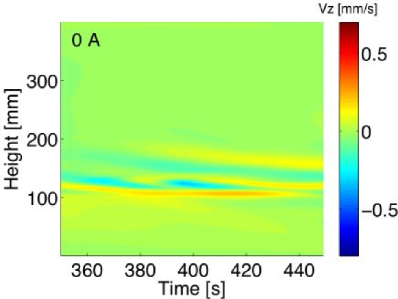
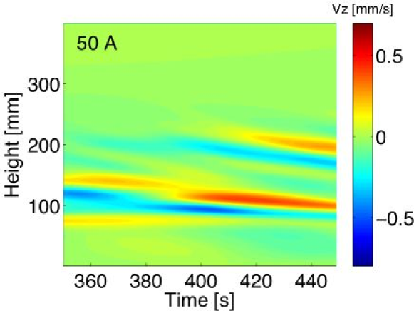
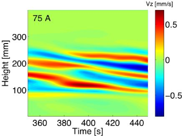
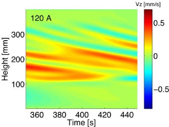
Background states with purely axial or purely azimuthal magnetic fields are symmetric under reflection $z\to-z$, but a helical field breaks this symmetryKnobloch (1996). As a result, growing modes in vertically infinite or periodic cylinders propagate axially in a unique direction: that of the background Poynting flux $-r\Omega B_{\theta}B_{z}/\mu_{0}$ Liu et al. (2006a). Fig. 2 displays vertical velocities near the outer cylinder in simulations corresponding to the experimental runs of Stefani et al. (2006) for several values of the toroidal current, $I_{\varphi}$. A wave pattern very similar to that in the experimental data is seen. It is most obvious for $I_{\varphi}=75\,{\rm A}$, just as in the experiment. Considering that we do not use exactly the same external coil configuration as PROMISE, the agreement is remarkably good (Table. 1).

Table 1: Comparison of results for the frequency, wavelength, axial phase speed, and amplitude obtained from simulation and experiment for the case $I_{\varphi}=75\,{\rm A}$. $f_{1}\equiv\Omega_{1}/2\pi$ is rotation frequency of inner cylinder.

	Calculation of Stefani et al. (2006); Rüdiger et al. (2006)	Experiment	Our Simulation
$f_{\rm wave}/f_{1}$	$\sim 0.14$	$\sim 0.15$	0.15
$\lambda_{wave}$ [cm]	$\sim 12$	6	6
$v_{p}$[$\,{\rm mm\;s^{-1}}$]	1.1	0.8	0.7
$A$[$\,{\rm mm\;s^{-1}}$]	unavailable	$\gtrsim 0.4$	$\gtrsim 0.6$

Interestingly, the jet becomes nearly steady when $I_{\varphi}\geq 50\,{\rm A}$. It is known that Ekman circulation is significantly modified when the Elsasser number $\Lambda\equiv B^{2}/(\mu_{0}\rho\eta\Omega)\gtrsim 1$Gilman (1971). If we use $|\boldsymbol{B}(r_{1})|$ for the field strength and $\Omega_{2}$ for $\Omega$ in this expression, then $\Lambda=4.8$ at $I_{\varphi}=75\,{\rm A}$.

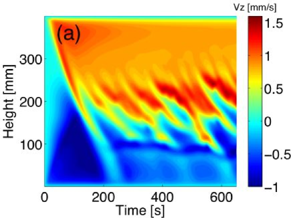
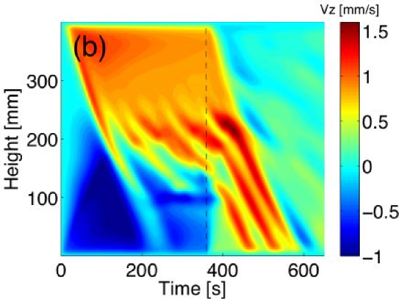
On the other hand, the magnetic field clearly promotes unsteadiness in the interior flow. The waves seen in Fig. 2 are probably related to HMRI, but we do not believe that they arise from a global instability of the experimental Couette flow. To demonstrate this, we have repeated the third ($I_{\varphi}=75\,{\rm A}$) simulation shown in Fig. 2 with different velocity boundary conditions. First, when we replace the rigidly rotating endcaps with differentially rotating ones that follow the ideal angular velocity profile of an infinitely long Taylor-Couette flow, then instead of the persistent travelling waves seen in Fig. 2, we see slowly damping standing waves, which we interpret as inertial oscillations excited by a small numerical force imbalance in the inital conditionsLiu et al. (2006a). Second, we perform a simulation that begins with the experimental boundary conditions until the traveling waves are well established, and then switches abruptly to ideal-Couette endcaps. After the switch, the Ekman circulation stops and the traveling waves disappear after one axial propagation time, as if they had been emitted by the Ekman layer at the upper endcap or by the layers on the upper part of the cylinders (Fig. 3). After the switch in boundary conditions but before the waves fully disappear, their vertical phase speed increases from $-0.7\,{\rm cm\;s^{-1}}$ to $-1.1\,{\rm cm\;s^{-1}}$; the latter is the speed predicted by linear analysis for axially periodic flow Rüdiger et al. (2006) (Fig. 3). Both numerical tests support the interpretation that the wave pattern observed in the simulation and in the experiment is not a global HMRI mode but rather a transient disturbance that is somehow excited by the Ekman circulation and then transiently amplified as it propagates along the background axial Poynting flux, but is then absorbed once it reaches the jet or the bottom end cap.

The authors would like to thank James Stone for the advice on the ZEUS code and thank Stephen Jardin for the advice of implementing full insulating boundary condition. This work was supported by the US Department of Energy, NASA under grants ATP03-0084-0106 and APRA04-0000-0152 and also by the National Science Foundation under grant AST-0205903.

References

- Balbus and Hawley (1998) S. Balbus and J. Hawley, Rev. Mod. Phys. 70, 1 (1998).
- Sisan et al. (2004) D. R. Sisan, N. Mujica, W. A. Tillotson, Y. Huang, W. Dorland, A. B. Hassam, T. M. Antonsen, and D. P. Lathrop, Phys. Rev. Lett. 93, 114502 (2004).
- Hollerbach and Rüdiger (2005) R. Hollerbach and G. Rüdiger, Phys. Rev. Lett. 95, 124501 (2005).
- Rüdiger et al. (2005) G. Rüdiger, R. Hollerbach, M. Schultz, and D. Shalybkov, Astron. Nachr. 326, 409 (2005).
- Stefani et al. (2006) F. Stefani, T. Gundrum, G. Gerbeth, G. Rüdiger, M. Schultz, J. Szklarski, and R. Hollerbach, Phys. Rev. Lett. 97, 184502 (2006).
- Rüdiger et al. (2006) G. Rüdiger, R. Hollerbach, F. Stefani, T. Gundrum, G. Gerbeth, and R. Rosner, Astrophys. J. 649, L145 (2006).
- Stefani et al. (2007) F. Stefani, T. Gundrum, G. Gerbeth, G. Rüdiger, J. Szklarski, and R. Hollerbach (2007), submitted to New J. Phys.
- Szklarski and Rüdiger (2006) J. Szklarski and G. Rüdiger, Astron. Nachr. 327, 844 (2006).
- Liu et al. (2006a) W. Liu, J. Goodman, I. Herron, and H. Ji, Phys. Rev. E 74, 056302 (2006a).
- Hayes et al. (2006) J. C. Hayes, M. L. Norman, R. A. Fiedler, J. O. Bordner, P. S. Li, S. E. Clark, A. ud Doula, and M.-M. M. Low., Astrophys, J. Suppl. 165, 188 (2006).
- Liu et al. (2006b) W. Liu, J. Goodman, and H. Ji, Astrophys. J. 643, 306 (2006b).
- Goodman and Ji (2002) J. Goodman and H. Ji, J. Fluid Mech. 462, 365 (2002).
- Müller and Bühler (2000) U. Müller and L. Bühler, Magnetohydrodynamic flows in ducts and cavities. (Springer-Verlag, 2000), chap. 3, page 39.
- Lackner (1976) K. Lackner, Comput. Phys. Comm. 12, p33 (1976).
- Grad and Rubin (1958) H. Grad and H. Rubin, Proceedings of the 2nd UN Conf. on the Peaceful Uses of Atomic Energy 31, 190. (1958).
- Shafranov (1966) V. Shafranov, Reviews of Plasma Physics 2, 103 (1966).
- Kageyama et al. (2004) A. Kageyama, H. Ji, J. Goodman, F. Chen, and E. Shoshan, J. Phys. Soc. Japan. 73, 2424 (2004).
- Knobloch (1996) E. Knobloch, Phys. Fluids 8, 1446 (1996).
- Gilman (1971) P. Gilman, Phys. Fluids 14, 7 (1971).