Far-infrared dust properties in the Galaxy and the Magellanic Clouds

Abstract

A recent data analysis of the far-infrared (FIR) map of the Galaxy and the Magellanic Clouds has shown that there is a tight correlation between two FIR colours: the $60~{}\mu{\rm m}-100~{}\mu{\rm m}$ and $100~{}\mu{\rm m}-140~{}\mu{\rm m}$ colours. This FIR colour relation called “main correlation” can be interpreted as indicative of a sequence of various interstellar radiation fields with a common FIR optical property of grains. In this paper, we constrain the FIR optical properties of grains by comparing the calculated FIR colours with the observational main correlation. We show that neither of the “standard” grain species (i.e. astronomical silicate and graphite grains) reproduces the main correlation. However, if the emissivity index at $100~{}\mu{\rm m}\la\lambda\la 200~{}\mu$m is changed to $\simeq 1$–1.5 (not $\simeq 2$ as the above two species), the main correlation can be successfully explained. Thus, we propose that the FIR emissivity index is $\simeq 1$–1.5 for the dust in the Galaxy and the Magellanic Clouds at $100~{}\mu{\rm m}\la\lambda\la 200~{}\mu{\rm m}$. We also consider the origin of the minor correlation called “sub-correlation”, which can be used to estimate the Galactic star formation rate.

1 Introduction

Dust grains absorb stellar ultraviolet (UV)–optical light and reprocess it into far-infrared (FIR), thereby affecting the energetics of interstellar medium (ISM) (e.g. Hirashita & Ferrara, 2002). The FIR luminosity is known to be a good indicator of star formation rate (SFR) in galaxies (Kennicutt, 1998; Inoue et al., 2000; Iglesias-Páramo et al., 2004). This can be explained if a large part of dust grains are heated by UV light from massive stars. The FIR spectral energy distribution (SED) of dust grains reflects various information on the grains themselves and on the sources of grain heating (e.g. Takeuchi et al., 2005; Dopita et al., 2005). Dust temperature, which can be estimated from wavelength at the peak of FIR SED, is determined by the intensity of the interstellar radiation field (ISRF) and the optical properties of dust (i.e. how it absorbs and emits light). Since dust grains absorb UV light efficiently, the FIR luminosity and the dust temperature mostly reflect the UV radiation field (Buat & Xu, 1996).

The FIR SED of the Galaxy (Milky Way) – the “nearest” galaxy – has been investigated by various authors. For example, Désert, Boulanger, & Puget (1990) and Dwek et al. (1997) explain the Galactic FIR SED as well as the extinction curve. Li & Greenberg (1997) provide a unified explanation for the Galactic polarization and extinction curve by adopting grains composed of silicate cores and organic refractory mantles, small carbonaceous particles, and polycyclic aromatic hydrocarbons (PAHs). Although there are some variations for assumed species, three grain components are usually assumed: silicate, graphite and PAHs. Besides the grain composition and the ISRF, the size distribution also affects the FIR SED. The temperature of silicate and graphite grains stays at an equilibrium temperature determined by the radiative equilibrium if the size is roughly larger than 0.01 $\mu$m (Draine & Anderson, 1985). Such large grains are called large grains (LGs). Since the equilibrium temperature is usually $\sim 15$–30 K in galactic environments, the emission peak lies around wavelengths of $\sim 100$–$200~{}\mu$m. If grains are smaller, they are transiently (stochastically) heated to a large temperature and emit photons with wavelengths shorter than $\sim 60~{}\mu$m (Draine & Anderson, 1985). Those grains are called very small grains (VSGs). The other component, PAH, only contributes to wavelengths shorter than $\sim 20~{}\mu$m. Since we are interested in wavelengths longer than $\sim 60$ $\mu$m, we do not treat PAHs in this paper.

So far, a major part of works have focused on FIR emission from high Galactic-latitude cirrus or from some limited regions in the Galactic plane (e.g. Dwek et al., 1997; Lagache et al., 1998). Because of the complication in the Galactic plane, which has large inhomogeneity with a variety of ISRF intensity and with a large range of gas (dust) density, etc., one may expect that a unified understanding of FIR SED in the Galactic plane is impossible. However, Hibi et al. (2006, hereafter H06) show that the FIR colour-colour relation (60–100 $\mu$m vs. 140–100 $\mu$m) defined by data points with Galactic latitudes of $|l|\leq 5^{\circ}$ has a clear sequence. A large fraction ($\sim 90$–95%) of the data points are on a colour-colour relation which they call “main correlation”. A minor part ($\sim 5$–10%) of points belong to another sequence called “sub-correlation” (see also Sakon et al., 2004, 2007). The sub-correlation tends to be found in regions with large radio intensity, which indicates a strong ISRF.

The “main correlation” of the Galactic plane is also consistent with the FIR colours of a sample of nearby galaxies compiled by Nagata et al. (2002) (see Fig. 8 of H06). In particular, the FIR colour-colour relation (60–100 $\mu$m vs. 140–100 $\mu$m) of the Magellanic Clouds is located at the extension of the main correlation of the Galactic plane. As stated by H06, this implies that the optical properties of grains in FIR are common among the Galaxy and the Magellanic Clouds. H06 also show that the FIR colours predicted by Li & Draine (2001) based on “standard” grain optical properties (Draine & Lee, 1984) cannot reproduce the main correlation.

Indeed, some observational and experimental results show that the FIR grain properties may be different from the “standard” ones. Based on the data of the Far-Infrared Absolute Spectrophotometer (FIRAS) aboard the Cosmic Background Explorer (COBE), Reach et al. (1995) suggest that the Galactic dust has more enhanced emissivity at $\lambda\ga 100~{}\mu$m than expected before. Some ISOPHOT observations have also reached a similar conclusion (del Burgo et al., 2003), although those observation target dense regions, where the dust properties may be modified by grain coagulation to form fluffy aggregates and/or by coating of ice mantles. Recently, Dobashi et al. (2005) have shown that the extinction at $V$ band derived from the FIR dust emission is higher than that derived from the optical Digitized Sky Survey data, suggesting a previous underestimation of dust emissivity at FIR wavelengths. An enhanced FIR emissivity is also derived for extragalactic objects (Dasyra et al., 2005). Agladze et al. (1996) find experimentally that some kinds of amorphous silicate show emissivities larger than those found in Draine & Lee (1984). Moreover, the wavelength dependence suggested by those authors is different from that presented by Draine & Lee (1984). Therefore, it is worth reexamining the FIR emissivity of dust by using the new observational results provided by H06.

The aim of this paper is to further investigate the origin of the main correlation both observationally and theoretically. Since the same main correlation is defined for the Magellanic Clouds, we also treat the FIR emission in these galaxies. Furthermore, we extend the analysis of H06 to high-Galactic-latitude regions to examine if the universality of the main correlation found in the Galactic plane holds over the entire Galaxy. Since the ISRF in high Galactic latitudes is considered to be more uniform than in the Galactic plane, the dependence on the Galactic latitude provides us with a key to understand the effect of inhomogeneous ISRF. A theoretical framework for the FIR SED developed by Draine & Li (2001, hereafter DL01) is adopted for theoretical analysis of the main correlation. The sub-correlation is also investigated.

This paper is organized as follows. First, in section 2, we describe the models adopted to calculate the FIR SED. Then, in section 3, we briefly review the observational results by H06, presenting also some additional analyses. In section 4, the FIR colour-colour relation predicted by our models is compared with the observational main correlation. Here, the sub-correlation is also discussed. Section 6 is devoted to the conclusion.

2 FIR SED Model

We adopt the theoretical framework of DL01 to calculate the SED of dust emission. Since we are interested in a wavelength range of $\lambda\sim 60$–140 $\mu$m, we neglect PAHs, which contribute to the emission at $\lambda\la 20~{}\mu$m (Dwek et al. 1997; DL01). Our assumptions on the relevant quantities are described below.

2.1 Interstellar radiation field

The ISRF in the solar neighborhood is used as the standard. The spectrum of the ISRF in the solar neighborhood is modeled by Mathis, Mezger, & Panagia (1983). The mean ISRF in the solar neighborhood integrated for all the solid angle is denoted as $4\pi J_{\lambda}^{\odot}$. Multiplying it with $\lambda$, Mathis et al. (1983) give the following numerical fitting in units of erg cm^-2 s^-1:

$$4\pi\lambda J_{\lambda}^{\odot}=\left\{\begin{array}[]{l}0~{}~{}~{}~{}~{}(\lambda_{\mu{\rm m}}\leq 0.0912)\\ 38.57\lambda_{\mu{\rm m}}^{4.4172}\\ ~{}~{}~{}~{}~{}~{}~{}(0.0912<\lambda_{\mu{\rm m}}\leq 0.110)\\ 2.045\times 10^{-2}\lambda_{\mu{\rm m}}\\ ~{}~{}~{}~{}~{}~{}~{}(0.110<\lambda_{\mu{\rm m}}\leq 0.134)\\ 7.115\times 10^{-4}\lambda_{\mu{\rm m}}^{-0.6678}\\ ~{}~{}~{}~{}~{}~{}~{}(0.134<\lambda_{\mu{\rm m}}\leq 0.246)\\ 4\pi\lambda_{\mu{\rm m}}[W_{1}B_{\lambda}(T_{1})+W_{2}B_{\lambda}(T_{2})+W_{3}B_{\lambda}(T_{3})]\\ ~{}~{}~{}~{}~{}~{}~{}(0.246<\lambda_{\mu{\rm m}})\,,\end{array}\right.$$ (10)

where $\lambda_{\mu{\rm m}}$ is the wavelength in units of $\mu$m, $B_{\lambda}(T)$ is the Planck function, $(T_{1},\,T_{2},\,T_{3})=(7500~{}{\rm K},\,4000~{}{\rm K},\,3000~{}{\rm K})$, and $(W_{1},\,W_{2},\,W_{3})=(1.0\times 10^{-14},\,1.0\times 10^{-13},\,4.0\times 10^{-13})$. The ISRF intensity $J_{\lambda}$ is scaled proportionally to $J_{\lambda}^{\odot}$ as follows:

$$J_{\lambda}=\chi J_{\lambda}^{\odot}\,,$$ (11)

i.e. the spectral shape of the ISRF is fixed and scaled with $\chi$ ($\chi=1$ corresponds to the ISRF intensity in the solar neighborhood).

2.2 Optical constants

We assume a grain to be spherical with a radius of $a$. The absorption cross section of the grain is expressed as $\pi a^{2}Q_{\rm abs}(\lambda)$, where $Q_{\rm abs}(\lambda)$ is called absorption efficiency. The optical constants of silicate and graphite grains are taken from Draine & Lee (1984). For the UV regime, we adopt “smoothed astronomical silicate” from Weingartner & Draine (2001) for silicate grains. For graphite grains, two-thirds of the particles have an dielectric function $\epsilon=\epsilon_{\bot}$ and one-third $\epsilon=\epsilon_{\parallel}$ (see Draine & Lee, 1984).

2.3 Grain size distribution

The number density of grains with sizes between $a$ and $a+{\rm d}a$ is denoted as $n_{i}(a)\,{\rm d}a$, where the subscript $i$ denotes a grain species ($i=\mbox{sil or gra}$ stands for silicate and graphite, respectively). We assume a power-law form for $n_{i}(a)$:

$$n_{i}(a)={\cal C}_{i}a^{-K}~{}~{}~{}(a_{\rm min}\leq a\leq a_{\rm max})\,,$$ (12)

where $a_{\rm min}$ and $a_{\rm max}$ are the upper and lower cutoffs of grain size, respectively, and ${\cal C}_{i}$ is the normalizing constant. Mathis, Rumpl, & Nordsieck (1977) find that the extinction curve observed in the solar neighborhood is reproduced by a composite model of graphite and silicate grains with $K=3.5$. We assume $a=3.5$ Å and $a_{\rm max}=0.25~{}\mu$m for both graphites and silicates (Mathis et al., 1977; Li & Draine, 2001), although Li & Draine (2001) adopt more elaborate functional form. We have confirmed that the difference does not affect the following discussion on the FIR colours.

The mixing ratio between silicate and graphite is uncertain and different even among models for the Galactic dust (Dwek et al., 1997; Takagi, Vansevičius, & Arimoto, 2003; Li & Draine, 2001). According to Pei (1992), the ratio between those two species is different among the Galaxy, the Large Magellanic Cloud (LMC) and the Small Magellanic Cloud (SMC). In the SMC, Pei (1992) suggest a silicate-dominated dust composition, while Welty et al. (2001) argue against such a composition from a study of the depletion pattern (but see Li, Misselt, & Wang, 2006). Considering such large uncertainty in the grain composition, we present the FIR SED of each grain species separately to avoid the uncertainty in the mixing ratio between the species. The effects of mixing two species are briefly mentioned in section 4.3.

As long as we treat the FIR colours of a single species (section 2.5), the constant ${\cal C}_{i}$ cancels out. Thus, it is not necessary to determine the absolute abundance of graphite and silicate. The relative ratio of ${\cal C}_{i}$ between species is important only when we consider a mixture of various species (section 4.3). In this case, ${\cal C}_{i}$ is determined by

$$\rho_{i}=\int_{a_{\rm min}}^{a_{\rm max}}\frac{4\pi}{3}a^{3}s_{i}{\cal C}_{i}a^{-K}\,{\rm d}a\,,$$ (13)

where $\rho_{i}$ is the mass density of species $i$ in the ISM, and $s_{i}$ is the material density of species $i$. We assume $s_{\rm sil}=3.3$ g cm^-3 and $s_{\rm gra}=2.2$ g cm^-3 (Jones, Tielens, & Hollenbach, 1996). In fact, we require only the ratio ${\cal C}_{\rm sil}/{\cal C}_{\rm gra}$ (or $\rho_{\rm sil}/\rho_{\rm gra}$) to calculate the FIR colors in a mixture of the two species.

2.4 Heat capacity

We adopt multi-dimensional Debye models for the heat capacity of grains. The heat capacity of a graphite grain per unit volume is (DL01; Takeuchi et al. 2003)

$$C_{\rm gra}=(N_{\rm C}-2)k_{\rm B}\left[f_{2}^{\prime}\left(\frac{T}{863~{}{\rm K}}\right)+2f_{2}^{\prime}\left(\frac{T}{2504~{}{\rm K}}\right)\right]\,,$$ (14)

$$f_{n}(x)\equiv n\int_{0}^{1}\frac{y^{n}{\rm d}y}{\exp(y/x)-1}\,,~{}~{}~{}f_{n}^{\prime}(x)\equiv\frac{\rm d}{{\rm d}x}f_{n}(x)\,,$$ (15)

where $N_{\rm C}=1.14\times 10^{23}$ cm^-3 (Takeuchi et al., 2003) is the number of carbon atoms contained in the unit volume of the grain, $k_{\rm B}$ is the Boltzmann constant, and $T$ is the grain temperature. The heat capacity of a silicate grain per unit volume is (DL01)

$$C_{\rm sil}=(N_{\rm a}-2)k_{\rm B}\left[2f_{2}^{\prime}\left(\frac{T}{500~{}{\rm K}}\right)+f_{3}^{\prime}\left(\frac{T}{1500~{}{\rm K}}\right)\right]\,,$$ (16)

where $N_{\rm a}=8.5\times 10^{22}$ cm^-3 is the number of atoms contained in the unit volume of the grain (Takeuchi et al., 2003).

2.5 Calculation of FIR colours

The total FIR intensity (per frequency per hydrogen nucleus per solid angle) of dust emission at a wavelength $\lambda$ can be estimated as

$$I_{\nu}^{i}(\lambda)=\int_{a_{\rm min}}^{a_{\rm max}}{\rm d}a\frac{1}{n_{\rm H}}n_{i}(a)\pi a^{2}Q_{\rm abs}(\lambda)\int_{0}^{\infty}{\rm d}T\,B_{\nu}(T)\frac{{\rm d}P_{i}}{{\rm d}T},$$

where $i$ specifies the grain species and ${\rm d}P_{i}/{\rm d}T$ is the temperature distribution function of the grains. We assume that the FIR radiation is optically thin. Thus, the observed colour directly reflects the ratio of the above intensity. Here the colour at wavelengths of $\lambda_{1}$ and $\lambda_{2}$ is defined as $I_{\nu}(\lambda_{1})/I_{\nu}(\lambda_{2})$, which is called $\lambda_{1}-\lambda_{2}$ colour.

The distribution function ${\rm d}P_{i}/{\rm d}T$ is calculated by the formalism of DL01 (see their section 4) based on the quantities in sections 2.1–2.4. The enthalpy of a grain is divided into discrete bins, and the transition probability between the bins is treated by taking into account the heating by interstellar radiation and the cooling by emission (see also Guhathakurta & Draine, 1989).

3 Data

3.1 Outline of the analysis by H06

The data analyzed by H06 are adopted in this paper. H06 used the Zodi-Subtracted Mission Average (ZSMA) taken by the Diffuse Infrared Background Experiment (DIRBE) of the COBE. They analyzed the data at three FIR wavelengths: $\lambda=60~{}\mu$m, 100 $\mu$m, and 140 $\mu$m. Then, they examined the relation between two colours, $I_{\nu}(60~{}\mu{\rm m})/I_{\nu}(100~{}\mu{\rm m})$ and $I_{\nu}(140~{}\mu{\rm m})/I_{\nu}(100~{}\mu{\rm m})$. Following H06, we adopt the intensity after colour correction for the 100-$\mu$m and 140-$\mu$m bands. For the Galactic plane, they treated regions with Galactic latitudes of $|b|<5^{\circ}$. The FIR data of the Magellanic Clouds are also analyzed. In order to avoid the uncertainty in the subtraction of the zodiacal component, they only select the region with $I_{\nu}(60~{}\mu{\rm m})>3$ MJy sr^-1. The error of $I_{\nu}$ is less than 10%.

In Figure 1a, we show the distribution of the Galactic-plane data in the colour-colour diagram. H06 found strong correlations between the two colours. More than 90% of the data lie on a strong correlation called main correlation, which can be fitted as (H06)

$$\frac{I_{\nu}(140~{}\mu{\rm m})}{I_{\nu}(100~{}\mu{\rm m})}=0.65\left(\frac{I_{\nu}(60~{}\mu{\rm m})}{I_{\nu}(100~{}\mu{\rm m})}\right)^{-0.78}\,.$$ (18)

The main correlation also explains the FIR colours of the LMC and the SMC (H06b). There is another correlation sequence, called sub-correlation in H06 (see also Hibi, 2006):

$$\frac{I_{\nu}(140~{}\mu{\rm m})}{I_{\nu}(100~{}\mu{\rm m})}=0.93\left(\frac{I_{\nu}(60~{}\mu{\rm m})}{I_{\nu}(100~{}\mu{\rm m})}\right)^{-0.56}\,.$$ (19)

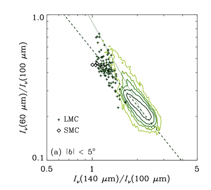
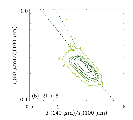
Figure 1: Far-infrared colour-colour ($60~{}\mu{\rm m}-100~{}\mu{\rm m}$ colour vs. $140~{}\mu{\rm m}-100~{}\mu{\rm m}$ colour) diagram derived from the COBE/DIRBE ZSMA map data. (a) The data of the Galactic plane ($|b|<5^{\circ}$), the LMC, and the SMC are shown. The contours show the distribution of the Galactic plane data. The contours show the levels where 50%, 80%, 90%, 95% and 99% of the data are contained. The LMC and SMC data are plotted with the filled circles and with the open diamonds, respectively. The dashed line and the dotted lines indicate the fittings for the main correlation and the sub-correlation, respectively. (b) Distribution of the data in high Galactic latutudes ($|b|>5^{\circ}$). The levels of the contours and the dashed and dotted lines are the same as those in Panel (a).

H06 also examined the dependence on the Galactic longitude $l$, showing that the FIR colours tend to shift downwards along the main correlation as $l$ increases from 0^∘ to 180^∘. Since the ISRF in the region toward the Galactic centre tends to be higher than that in the opposite direction (Mathis et al., 1983), the colour shift along the main correlation can be caused by the difference in ISRF; that is, the FIR colours of dust grains irradiated by a high ISRF tends to be situated in an upper part of the main correlation on the colour-colour diagram.

We extend our analysis to high Galactic latitudes ($|b|>5^{\circ}$). The procedure of the data analysis and the selection criterion for the intensity (i.e. $I_{\nu}(60~{}\mu{\rm m})>3$ MJy sr^-1) are the same as H06. Most of the data are taken from $|b|\la 40^{\circ}$, since the criterion for the intensity is hard to be satisfied in higher Galactic latitudes. In Figure 1b, we show the results. Although the data distribution is shifted slightly downward compared with the Galactic plane data, we clearly see the main correlation. Moreover, the sub-correlation is not clear in the high Galactic latitudes. This supports the idea of H06 that the sub-correlation is produced by the contamination of high-ISRF regions, which tend to reside in the Galactic plane.

3.2 The main correlation

The data presented in Figure 1 indicate that the main correlation is robust against the change of Galactic latitudes ($b$). H06 also show that the FIR colours shifts along the main correlation by the variation of Galactic longitudes ($l$). These facts mean that the main correlation is independent of the complexity of the Galactic structure. Since the inhomogeneity of ISRF should be smaller in high Galactic latitudes than in the Galactic plane, the robustness of the main correlation over a variety of $b$ suggests that a detailed modeling of galactic structures and of inhomogeneous ISRF are not necessary to understand the main correlation.

As mentioned in the previous subsection, H06 argued that the main correlation is produced by a sequence of varying ISRF: the FIR colours tend to be located in an upper part of the main correlation for a high ISRF. However, this was only suggested from the longitude dependence but was not theoretically demonstrated. Thus, in section 4, we investigate how the FIR colour-colour relation changes for various ISRF intensities. By examining if the observed colour-colour relation is explained or not, we will finally be able to test what kind of grain species is consistent with the observational FIR colour-colour relation (section 5.1).

It is worth noting that the main correlation can also explain the FIR colours in the Magellanic Clouds. Since the LMC has a face-on geometry, the inhomogeneity in the ISRF in a line of sight may be small. The fact that the FIR colour-colour relation of the LMC shifts upward relative to that of the Galaxy suggests that the location in the main correlation reflects the strength of ISRF, since the LMC is generally believed to have a higher ISRF than the Galaxy (e.g. Fukui, 2001; Tumlinson et al., 2002). It is surprising that the FIR colours of the LMC and the SMC are located on the main correlation defined by the Galactic dust grains, and it is interesting to give a unified understanding of the FIR colours for those three galaxies. We also tackle this problem in sections 4 and 5.

3.3 The sub-correlation

H06 show that the sub-correlation can be reproduced by summing two colours in the main correlation. Thus, they argue that the main correlation is fundamental. We also follow their argument and concentrate on explaining the main correlation. The sub-correlation is investigated in section 5.2.

4 Results

4.1 Standard grain optical constants

From various observational evidence such as extinction curves and interstellar depletion patterns, dust is believed to be mainly composed of two species: silicate and carbonaceous dust (Mathis, 1990; Li & Greenberg, 1997; Jones, 2000; Okada et al., 2006). For those two species, Draine & Lee (1984) proposed astronomical silicate and graphite, which reproduce the observational extinction curve and FIR emission spectrum (see also Li & Draine, 2001).

Based on the models described in section 2, we examine how the FIR colours change by the variation of ISRF ($\chi$). Following H06, we focus on the relation between the 60 $\mu$m–100 $\mu$m colour [$I_{\nu}(60~{}\mu{\rm m})/I_{\nu}(100~{}\mu{\rm m})$] and the 140 $\mu$m–100 $\mu$m colour [$I_{\nu}(140~{}\mu{\rm m})/I_{\nu}(100~{}\mu{\rm m})$]. In Figures 2, we plot the colour-colour relations of graphite and astronomical silicate for $\chi=0.3$, 1, 3, 10, and 30. The discrepancy between the observational main correlation and the theoretical prediction is significant. Some mechanism that shifts the colour-colour relation upward and/or rightward should be included to explain the observational colour correlations.

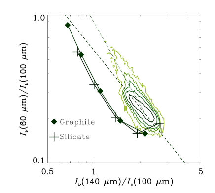
Figure 2: FIR colour-colour ($60~{}\mu{\rm m}-100~{}\mu{\rm m}$ vs. $140~{}\mu{\rm m}-100~{}\mu{\rm m}$) relation for silicate and graphite grains (large crosses and large squares,respectively). The different points correspond to $\chi=0.3$, 1, 3, 10, and 30 from low to high $140~{}\mu{\rm m}-100~{}\mu{\rm m}$ colours. The same contour as shown in Figure 1a as well as the main and sub-correlations (dashed and dotted lines, respectively) are also presented.

It should be noticed that both silicate and graphite grains trace similar tracks on the FIR colour-colour relation although the UV absorption coefficients and heat capacities are different between those two species. This strongly suggests that the track on the FIR colour-colour diagram is determined mainly by the FIR absorption coefficients of grains. Indeed, both have dependence roughly described as $Q_{\rm abs}\propto\lambda^{-2}$. Thus, we suspect that the FIR colour-colour relation is not sensitive to various factors other than the wavelength dependence of the FIR absorption coefficient.

The colour-colour relation shifts upwards if the contribution from VSGs relative to that of LGs increases, since the emission from stochastically heated VSGs contributes significant to the emission at $\lambda=60~{}\mu$m. Indeed, grains with $a\sim 50$ Å contribute to the 60 $\mu$m intensity (Draine & Li, 2007). A change of the ISRF spectrum and/or of the grain size distribution can change the relative contribution from the stochastic VSG emission. First we vary the ISRF spectrum. A hard spectrum could relatively enhance the emission from VSGs, since the cross section of a VSG is sensitive to the change of wavelength in the UV regime (e.g. Draine & Lee, 1984). We calculate the FIR colours by assuming a “hard” spectrum without the optical–NIR bump; i.e. we adopt $7.115\times 10^{-4}\lambda_{\rm\mu m}^{-0.6678}$ for $\lambda_{\rm\mu m}>0.246$ instead of the expression in equation (10). The FIR colour-colour relation calculated with this hard spectrum is shown in Figure 3a. The colour-colour relation shifts upward and approaches the main correlation compared with the relation in Figure 2. This is due to relative enhancement of the stochastic heating of VSGs, which contributes to the 60 $\mu$m emission. However, the change of the FIR colours for various $\chi$ does not follow the main correlation. Moreover, such a hard spectrum as assumed here is unrealistic for high Galactic latitude, where the main correlation is also seen. Thus, we conclude that the change of the UV spectrum cannot explain the observational FIR colours.

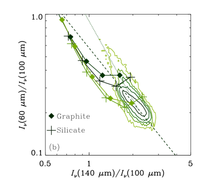
Figure 3: Same as Figure 2 but for (a) the hard ISRF and (b) the size distribution of grains with $K=3.75$ and 4.0 (lower and upper sequences, respectively).

The enhancement of the stochastic heating occurs also if the relative number of VSGs increases. Thus, we expect that the colour-colour relation shifts upward if we assume a grain size distribution with an enhanced number of VSGs. The number of VSGs may be increased by shattering (Jones et al., 1996). The size distribution shown by Jones et al. (1996) can be roughly fitted by $n(a)\propto a^{-4.0}$ (i.e. $K=4.0$ in equation 12). We also examine $K=3.75$ as an intermediate case. In both cases, we adopt the same values of $a_{\rm min}$ and $a_{\rm max}$ as assumed in section 2.3. In Figure 3b, we show the colour-colour relation for $K=3.75$ and 4.0. We observe that the 60 $\mu$m–100 $\mu$m colour is sensitive to the grain size distribution. However, the overall trend of the main correlation is not reproduced neither by $K=3.75$ nor by $K=4.0$. The 60 $\mu$m–100 $\mu$m colour is clearly out of the observed range for $K=4.0$. Although $K=3.75$ explains the most concentrated part of the data with $\chi\sim 0.3$–1, the trend along the main correlation is not reproduced.

The upper and lower cutoffs of grain size ($a_{\rm max}$ and $a_{\rm min}$) can also be changed. However, the 140 $\mu$m–100 $\mu$m colour is not sensitive to the change of $a_{\rm min}$ because it is determined by the equilibrium temperature of large grains. It is not largely affected by the change of $a_{\rm max}$ as long as $a_{\rm max}\ga 0.1~{}\mu$m. The 60 $\mu$m–100 $\mu$m colour monotonically increases if the fraction of VSGs increases. According to Draine & Li (2007), grains with $a\sim 50$ Å contribute to the 60 $\mu$m flux, while a large fraction of the 100 $\mu$m flux comes from grains with $a\ga 100$ Å. Thus, as $a_{\rm min}$ decreases and/or $a_{\rm max}$ decreases, the 60 $\mu$m–100 $\mu$m colour monotonically increases. However, this colour is not sensitive to the grain size distribution at $a\ll 50$ Å, and the abundance of such very small particles is constrained better in mid-infrared (e.g. Sakon et al., 2007). We have confirmed after calculations with our models that resulting colour-colour relations predicted by decreased $a_{\rm min}$ and/or $a_{\rm max}$ are similar to those in Figure 3 and that the observed main correlation can never be explained by changes of $a_{\rm min}$ and $a_{\rm max}$.

In summary, it is difficult to explain the overall main correlation by simply enhancing the stochastic heating component, which contributes to the 60 $\mu$m intensity. Heat capacities and grain optical constants are also concerned with the FIR SED. However, as shown in Appendix A, difference in the heat capacity does not change the FIR colour-colour relation. There, we also show that different materials with different UV–near-infrared absorption coefficients does not explain the observational FIR colour-colour relation. We note that all the materials examined in Appendix A have the FIR spectral index (which is defined as $\beta\equiv-{\rm d}\ln Q_{\rm abs}(\lambda)/{\rm d}\ln\lambda$, i.e. $Q_{\rm abs}$ is approximated to be proportional to $\lambda^{-\beta}$) nearly equal to 2. We are left with changing the FIR optical properties of grains. The following subsection is devoted to examining the possibility that the FIR spectral index is different from 2.

4.2 Dependence on the FIR emissivity index

A spectral index $\beta=2$ is the most frequently used value, which is supported by some experiments and observations (e.g. Hildebrand, 1983; Draine & Lee, 1984). On the other hand, an analysis of the FIRAS data by Wright et al. (1991) indicates that the Galactic dust has $\beta\simeq 1.65$. Some other observational and experimental results also indicate that the FIR emissivity index may be smaller than 2 (Reach et al., 1995; Aguirre et al., 2003). The range of $\beta$ is roughly from $\sim 0.9$ to 1.6 as suggested for the FIR colours of the Galaxy and the Magellanic Clouds (Reach et al., 1995; Aguirre et al., 2003). Some species indeed show such a low emissivity index (Agladze et al., 1996): $\beta\simeq 1.2$ for ${\rm MgO}\cdot 2{\rm SiO}_{2}$ (amorphous). Since there is no available information on the optical constants of ${\rm MgO}\cdot 2{\rm SiO}_{2}$ in the wavelengths shorter than FIR, we cannot include this species consistently into our models. Fortunately, the resulting FIR colours are not sensitive to the detailed wavelength dependence of the UV absorption coefficient as shown in Appendix A. Thus, we adopt the emissivity of astronomical silicate or graphite at $\lambda\leq 100~{}\mu$m and change the spectral index at $\lambda>100~{}\mu$m. That is, we choose the following absorption efficiency for $\lambda>100~{}\mu{\rm m}$:

$$Q_{\rm abs}(\lambda,\,\beta)=Q_{\rm abs}(\lambda=100~{}\mu{\rm m})\left(\frac{\lambda}{100~{}\mu{\rm m}}\right)^{-\beta}\,,$$ (20)

where we adopt the value $Q_{\rm abs}(\lambda=100~{}\mu{\rm m})$ from Draine & Lee (1984) for astronomical silicate and graphite.

In Figure 4, we show the colour-colour relation for various FIR spectral indexes. Here we call the species according to the adopted optical properties at $\lambda<100~{}\mu{\rm m}$ although we modify artificially $Q_{\rm abs}$ at $\lambda>100~{}\mu{\rm m}$. We observe from Figure 4 that $\beta=1$ is roughly consistent with the main correlation if the ISRF intensity is between $\sim 1$ and $\sim 10$ ($\beta=1.5$ may also be permitted considering the uncertainty in the data). It is worth noting that the colour-colour relation is just along the main correlation. Moreover, the region of the largest concentration of the data (see the contours in Fig. 4) is reproduced with a standard ISRF $\chi\sim 1$. Thus, we conclude that a FIR emissivity index of $\sim 1$–1.5 is successful in reproducing the main correlation.

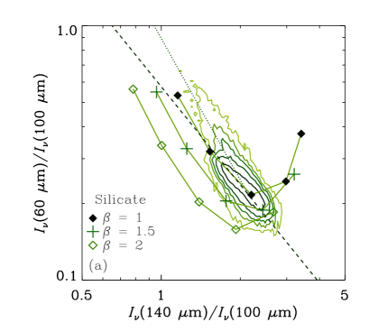
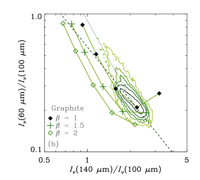
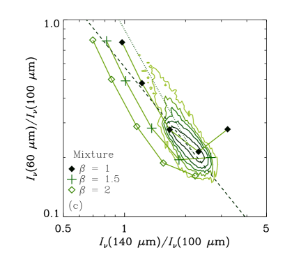
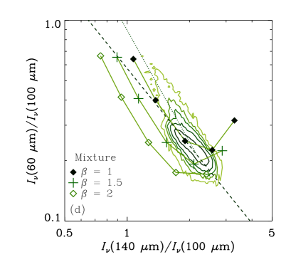
Figure 4: Same as Figure 2 but for various FIR emissivity indexes $\beta$ defined at $\lambda\geq 100~{}\mu$m. The filled squares, crosses, and open squares show the FIR colour-colour relation for $\beta=1$, 1.5, and 2, respectively. In Panels (a) and (b), we assume the silicate and graphite absorption efficiencies at $\lambda<100~{}\mu$m, respectively. In Panel (c) and (d), the colours-colour relation of the graphite-silicate mixture is shown, where the mass ratios between silicate and graphite are 1.11 : 1 and 7.25 : 1, respectively.

For the absorption efficiency at $\lambda>100~{}\mu$m, we also examine a hybrid functional form proposed by Reach et al. (1995):

$$Q_{\rm abs}(\lambda)=\frac{(\lambda/\lambda_{0})^{-2}}{[1+(\lambda_{1}/\lambda)^{6}]^{1/6}}\,,$$ (21)

which behaves like equation (20) with $\beta=1$ for $\lambda\ll\lambda_{1}$ and $\beta=2$ at $\lambda\gg\lambda_{1}$ (see also Bianchi, Davies, & Alton, 1999). We assume that $\lambda_{1}=200~{}\mu$m, following Reach et al. (1995). For $\lambda\leq 100~{}\mu$m, we adopt the same absorption efficiency of astronomical silicate and graphite as used in section 4.1. Thus, we set the value of $\lambda_{0}$ so that the continuity of $Q_{\rm abs}$ at $100~{}\mu$m is satisfied. In Figure 5, we show the colour-colour relation for this absorption efficiency. The resulting relation is similar to that in Figure 4 with $\beta=1$. Thus, the 60 $\mu$m–100 $\mu$m vs. 140 $\mu$m–100 $\mu$m colour-colour relation is determined by the spectral index around $\lambda\sim 100~{}\mu$m–140 $\mu$m and is not sensitive to the details of the absorption coefficient at the other wavelengths.

4.3 Silicate-graphite mixture

In reality, both silicate and graphite contribute to the FIR SED at the same time. Thus, it is worth examining the FIR colour-colour relation predicted by mixtures of those two species. As stated in section 2.3, there is a large uncertainty in the mixing ratio among models. Thus, we examine a variety of mixing ratios. In Figure 4c, we show the FIR colour-colour relation calculated by a graphite-silicate mixture. First, the mass ratio of those two species is assumed to be $\rho_{\rm sil}/\rho_{\rm gra}=1.11$ according to Takagi et al. (2003). With this ratio, graphite dominates the FIR SED and the FIR colour-colour relation becomes almost the same as that of graphite (see Figure 4b). A similar graphite-dominated FIR SED can be seen in Dwek et al. (1997). As the fraction of silicate becomes larger, the FIR colour-colour relation approaches that shown in Figure 4a. In order to show this, we also examine a silicate-dominated composition as proposed for the LMC. We adopt a mass ratio of $\rho_{\rm sil}/\rho_{\rm gra}=7.25$. The result is shown in Figure 4d, which becomes relatively similar to the silicate colours shown in Figure 4a. However, it is evident that the colours of the mixed population are between those of single species.

5 Discussion

5.1 Grain optical properties in FIR

We have found in the previous section that the FIR colours are sensitive to the FIR absorption coefficient of dust grains and are robust to the absorption coefficient in wavelengths other than the FIR. Then we have suggested that the FIR emissivity index of $\simeq 1$ fits the main correlation. An emissivity index of $\beta\sim 1$ can also explain the submillimetre part of the Galactic FIR SED without introducing a very cold component (Reach et al., 1995). Indeed it would be possible to explain the FIR colour by mixing two components with different dust temperatures, but the robustness of the main correlation against the Galactic latitudes would strongly require that the mixing ratio between those two components be uniform over the entire Galaxy. More natural interpretation is obviously that the main correlation reflects the FIR absorption coefficient of dust grains itself. Thus, it is important to investigate what kind of the FIR absorption coefficients reproduces the observational main correlation.

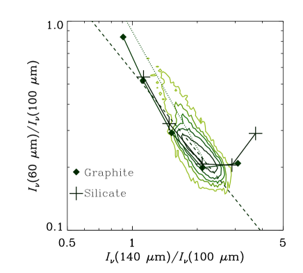
Figure 5: Same as Figure 2 but for the FIR emissivity shown by equation 21.

We note that we cannot strongly constrain the spectral index at wavelength out of the range treated in this paper and that we do not reject the possibility that the spectral index varies as a function of wavelength as we examined in equation (21). In most of the previous works on the Galactic FIR spectra, within the uncertainty, the FIR SED at $60~{}\mu{\rm m}\la\lambda\la 200~{}\mu{\rm m}$ was fitted quite well both by $\beta=2$ and by $\beta=1$ with different dust temperatures. However, since the analysis adopted in this paper (H06) only uses the pixels with negligible uncertainty ($<10\%$), we are able to constrain the FIR dust emissivity index more strongly than previous works, based on the strong correlation called main correlation.

Also for extragalactic objects, the FIR spectral index is a matter of debate. The FIR–submillimetre (sub-mm) SEDs of dust-rich galaxies such as spiral galaxies usually show an excess in the sub-mm regime relative to a single component fit to the FIR regime. This is usually interpreted as existence of very cold dust contributing to the sub-mm emission (e.g. Stevens, Amure, & Gear, 2005). However, it is also important to stress that the discussion on the amount of very cold dust strongly depends on the assumed FIR–sub-mm spectral index. The excess of the sub-mm emission could be explained by a small spectral index ($\beta$). Kiuchi et al. (2004) show that the FIR–sub-mm SEDs of some galaxies can be fitted with $\beta\simeq 1$–1.5, similar to our derived values.

As shown by H06, the main correlation is also consistent with the FIR colours of nearby galaxies. This implies that investigating the origin of the main correlation is of a general significance to the interpretation of the FIR colours in extragalactic objects.

5.2 Origin of the sub-correlation

H06 propose that the sub-correlation shown by the dotted line in Figure 1 can be explained by mixing two colours in the main correlation. Such a mixture of FIR colours in a line of sight is called overlap effect in H06. H06 also show observationally that the sub-correlation tends to be associated with lines of sight with a high ISRF intensity indicated by a strong radio continuum intensity. Thus, the sub-correlation may be reproduced by a contamination of a FIR colour with a high radiation field intensity.

In order to investigate the overlap effect in our framework, we assume a two-component model, in which two FIR colours calculated with two different radiation field intensities ($\chi$) are mixed. Such a superposition of FIR colours is treated by Onaka et al. (2007) in a more sophisticated manner, but our simple approach has an advantage that the physical quantities are easy to interpret. We denote the FIR intensity predicted under an ISRF intensity of $\chi$ as $I_{\nu}(\lambda;\,\chi)$. Then, we examine a two-component model in which the FIR intensity is composed of a mixture of two ISRF $\chi_{1}$ and $\chi_{2}$ $(\chi_{1}<\chi_{2})$, $I_{\nu}(\lambda;\,\{\chi_{1},\,\chi_{2}\},f_{2})$:

$$I_{\nu}(\lambda;\,\{\chi_{1},\,\chi_{2}\},f_{2})=(1-f_{2})I_{\nu}(\lambda;\,\chi_{1})+f_{2}I_{\nu}(\lambda;\,\chi_{2})\,,$$ (22)

where $f_{2}$ is the contributing fraction of the component with $\chi=\chi_{2}$ in the line of sight. Since the FIR emission is optically thin, the contribution from each component is proportional to the dust optical depth. Thus, if the total dust optical depth at wavelength $\lambda$ is $\tau$, $f_{2}\tau$ is occupied with a component with $\chi=\chi_{2}$.

We adopt the FIR absorption efficiency expressed by equation (20) with $\beta=1$, since it explains the main correlation (section 4.2; Figure 4b). We adopt the graphite species for the absorption efficiency at $\lambda<100~{}\mu$m. If we adopt the silicate absorption efficiency at $\lambda<100~{}\mu$m, we obtain similar results, and the following discussions are valid. We fix $\chi_{1}=1$ as a general ISRF and examine various $\chi_{2}(>1)$ and $f_{2}$ as a contaminating high radiation field. In Figure 6, we show the results. We find that the main correlation shifts rightward (i.e. toward the sub-correlation) on the colour-colour diagram if we mix two colours with different $\chi$. From Figure 6, if about 10% of the total column of a line of sight is filled with a high-$\chi$ region, the sub-correlation is reproduced. In the following, we discuss the filling factor assuming that the high radiation field originates from young massive stars.

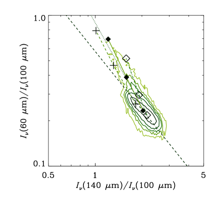
Figure 6: Same as Figure 2 but for the two-component models with $\chi_{1}=1$ and $\chi_{2}=3$, 10, and 30 (lower to upper points). The filling factors of the second component ($f_{2}$) are assumed to be 0.3, 0.1, and 0.03 for the crosses, filled squares, and open squares, respectively.

We consider typical star-forming regions containing OB stars as regions with a high radiation field. Hirashita et al. (2001) show that a typical Galactic H ii region emit ionizing photons at a rate of $3.0\times 10^{49}$ s^-1. If we assume that the mean energy of the ionizing photons is 15 eV (Inoue et al., 2000), the luminosity of the ionizing photons from the star-forming region becomes $1.9\times 10^{5}~{}L_{\odot}$. Assuming that the luminosity of nonionizing photons is 1.5 times as large as that of the ionizing UV photons (Inoue et al., 2000), we obtain the nonionizing UV luminosity of the star-forming region, $\ell_{\rm UV}$, as $2.8\times 10^{5}~{}L_{\odot}$. We assume that the nonionizing photons contribute to the dust heating (Buat & Xu, 1996; Inoue et al., 2000) and treat the whole stellar cluster as a point source. Then, the UV radiation flux ($f_{\rm UV}$) at a distance of $r$ from the centre of the star-forming region can be estimated as

$$f_{\rm UV} = \frac{\ell_{\rm UV}\,e^{-\tau_{\rm UV}}}{4\pi r^{2}}$$ (23)

$$= 9.0\times 10^{-2}\left(\frac{r}{10~{}{\rm pc}}\right)^{-2}e^{-\tau_{\rm UV}}~{}{\rm erg~{}s^{-1}~{}cm^{-2}}\,,$$

where $\tau_{\rm UV}$ is the optical depth of dust grains in the UV regime. On the other hand, integrating equation (10) over the UV regime ($\lambda=912$–4000 Å), we obtain the UV flux as $f_{\rm UV}=2.89\times 10^{-3}\chi$ erg s^-1 cm^-2 (we used $7.115\times 10^{-4}\lambda_{\mu{\rm m}}^{-0.6678}$ for $\lambda_{\mu{\rm m}}>0.246$). Equating this with equation (23), we obtain

$$\chi=31\left(\frac{r}{10~{}{\rm pc}}\right)^{-2}e^{-\tau_{\rm UV}}\,.$$ (24)

The UV optical depth ($\tau_{\rm UV}$) is related to the UV extinction in units of magnitude ($A_{\rm UV}$) as $\tau_{\rm UV}=A_{\rm UV}/1.086$. If we take $\lambda=2000$ Å as a representative value of the UV wavelengths (Hirashita, Buat, & Inoue, 2003), we obtain $A_{\rm UV}=E_{B-V}(5.52+R_{V})=8.60E_{B-V}$ for the Galactic extinction curve (Pei, 1992), where $E_{B-V}$ is the colour excess defined between the $B$ and $V$ bands ($E_{B-V}\equiv A_{B}-A_{V}$), and $R_{V}\equiv A_{V}/E_{B-V}$ ($A_{\lambda}$ is the extinction at a wavelength of $\lambda$). The ratio between the hydrogen column density (both in atomic and molecular form) and $E_{B-V}$ is estimated as $N_{\rm H}/E_{B-V}=5.8\times 10^{21}$ cm^-2 mag^-1 in the Galactic environment (Bohlin, Savage, & Drake, 1978). Combining the above expressions, we finally obtain the relation between $\tau_{\rm UV}$ and $N_{\rm H}$ as $\tau_{\rm UV}=N_{\rm H}/(7.32\times 10^{20}~{}{\rm cm}^{-2})$.

Hirashita et al. (2001) assume that the number density of hydrogen nuclei in a star-forming region is typically $n_{\rm H}=10^{2}$ cm^-3. Adopting the same number density, we estimate that $N_{\rm H}=n_{\rm H}r$ (with $n_{\rm H}=10^{2}$ cm^-3) around a star-forming region. In Figure 7, we show the ISRF as a function of $r$. The sharp decline at $r\ga 5$ pc is due to the dust extinction. Although Hirashita et al. (2001) focused on H ii regions with typical stellar ages less than $\sim 10^{7}$ yr, stars with lifetimes of $\sim 10^{8}$ yr (B-type stars) also emit UV radiation (e.g. Hirashita et al., 2001). Such UV emitting stars with long lifetimes, after dispersal of dense regions after $\sim 10^{7}$ yr, may be found in the field where the ISM density is roughly $\sim 1$ cm^-1. Thus, we also investigate the radiation field with $n_{\rm H}=1$ cm^-3. In this case, the radiation field declines as $r^{-2}$ and the dust extinction is negligible up to $r\sim 100$ pc as shown in Figure 7.

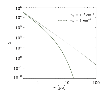
Figure 7: ISRF normalized to the solar neighborhood value, $\chi$, as a function of the distance from the center of the star-forming region, $r$. The solid and dotted lines correspond to the results with $n_{\rm H}=10^{2}$ cm^-3 and 1 cm^-3, respectively.

H06 have shown that the FIR colour-colour relation follows the sub-correlation in $\sim 5$–10% of the lines of sight in the Galactic plane. The probability (denoted as $P(r)$) that an arbitrary line of sight along the Galactic plane passes through a region with a radius of $r$ can be estimated by $P(r)\simeq\pi r^{2}sN_{\rm SF}/(\pi R_{\rm d}^{2}2H_{\rm d})$, where $s$ is the path length, $H_{\rm d}$ is the scale height of the Galactic disk, and $N_{\rm SF}$ is the number of the regions in the entire Galaxy. Taking $s\sim R_{\rm d}$, we obtain

$$P(r) \sim 0.13\left(\frac{r}{5~{}{\rm pc}}\right)^{2}\left(\frac{N_{\rm SF}}{10^{4}}\right)\left(\frac{R_{\rm d}}{10~{}{\rm kpc}}\right)^{-1}$$ (25)

$$\times \left(\frac{H_{\rm d}}{100~{}{\rm pc}}\right)^{-1}\,.$$

This probability is possibly dependent on the line of sight through the density structure in the Galactic plane such as spiral arms, vertical stratification, etc. However, the above probability is valid if we take a large number of lines of sight in the Galactic plane as H06 have done. The estimate of $N_{\rm SF}$ in terms of the Galactic SFR (or OB star luminosity) is presented in Appendix B, and the typical SFR (or OB star luminosity) of the Galaxy gives $N_{\rm SF}\sim 8\times 10^{3}$.

The above probability estimated in equation (25) is comparable to the fraction of sightlines with the sub-correlation if $r\sim 5$ pc. If the sub-correlation is associated with regions near massive stars, the sub-correlation passes through a region whose typical distance from young stars is 5 pc. From Figure 7, the radiation field at $r\sim 5$ pc from massive stars is typically $\chi\sim 10$–100. Thus, in order to explain the sub-correlation, it would be necessary to consider a mixture of two FIR colours: one with $\chi\sim 1$ as a normal diffuse ISRF and the other with $\chi\sim 10$–100 as a radiation field near massive stars. This is roughly consistent with the mixture of the two components examined above and in Figure 6.

6 Conclusion

The observational main correlation between the 60 $\mu$m–100 $\mu$m colour and the 140 $\mu$m–100$\mu$m colour found by H06 is not explained by the previous models. We have examined changes of quantities concerning the FIR SED. The most concentrated region in the colour-colour diagram and the trend along the main correlation cannot be explained neither by the change of the ISRF spectrum nor by the the variation of the grain size distribution. The FIR colour-colour is not very sensitive to the heat capacity and the detailed wavelength dependence of the UV absorption coefficient.

On the other hand, we find that the FIR colour-colour relation is sensitive to the FIR absorption coefficient, in particular to the emissivity index $\beta$ defined in equation (20). The observational main correlation is consistent with the theoretical FIR colours if we assume that $\beta\simeq 1$–1.5 around 100–200 $\mu$m. This is different from the spectral index often assumed for astronomical silicate and graphite species ($\beta\simeq 2$). Indeed some observational and experimental works suggest that the FIR spectral index is significantly smaller than 2 and may be nearly 1 (e.g. Reach et al., 1995; Agladze et al., 1996). The difference in the FIR emissivity affects the estimate of dust mass and of dust temperature. Thus, we should further examine the FIR dust properties not only of the Galaxy but also of extragalactic objects by reexamining FIR data. New data taken by the Spitzer Space Telescope (Werner et al., 2004) and the AKARI (Murakami, 2004; Shibai, 2004; Matsuhara et al., 2006), both of which have a FIR band with $\lambda>100~{}\mu$m, are suitable for such a purpose.

We have also considered the origin of the sub-correlation by taking into account the overlap effect; that is, the FIR radiation comes from regions with a variety of UV radiation field intensity. For simplicity, we assume a mixture of two components illuminated by different UV radiation fields: one is a normal diffuse component with $\chi\sim 1$ and the other is an intense field near to young massive stars ($\chi\sim 10$). As a result, we have found that the sub-correlation can be understood by the FIR colour with high $\chi$ contaminated by that with normal $\chi(\sim 1)$. This explains the observational fact that the sub-correlation is associated with the regions with intense radiation field (H06). Indeed, we have also shown that the observed fraction of the data points on the sub-correlation is consistent with the total luminosity (or number) of OB stars in the Galaxy.

Appendix A Material Dependence

A.1 Optical constants

Among silicate species, olivine and pyroxene are often considered as promising candidates of astronomical grains (e.g. Dorschner et al., 1995). Since the optical constants are different among species, we examine the robustness of the predicted FIR colour-colour relation against the change of materials. As for olivine, the optical constants of two compositions are available: Mg_2yFe_2-2ySiO₄ with $y=0.4$ and 0.5 for $\lambda=0.20$–500 $\mu$m (Dorschner et al., 1995). The optical constants at $\lambda>500~{}\mu$m do not affect our results because of small absorption efficiency, but those at $\lambda<0.20~{}\mu$m may be important, since the absorption of UV radiation determines the dust temperature. For both $y=0.4$ and 0.5, we adopt the optical constants of olivine derived by Huffman & Stapp (1973) at $\lambda<0.20~{}\mu$.

We calculate the FIR colour-colour ($I(60~{}\mu{\rm m})/I(100~{}\mu{\rm m})$ vs. $I(140~{}\mu{\rm m})/I(100~{}\mu{\rm m})$) relation by adopting the above optical constants. The other quantities adopted are the same as those in the text. As a result, we find that the FIR colour-colour relation of the above materials is the same as that of astronomical silicate within the error of the colour-colour relation. Thus, olivine is not successful in reproducing the main correlation. If we adopt the optical constants of pyroxene found in Dorschner et al. (1995) (but we use the olivine optical constants in Huffman & Stapp (1973) for $\lambda<0.2~{}\mu$m), the main correlation is not reproduced. Thus, as far as we examined here, we conclude that silicate does not explain the observational FIR colour-colour relation.

We have examined other materials (FeO, Fe₃O₄, SiO₂, and MgO) that can be included in silicates by using the optical constants adopted in Hirashita et al. (2005). We also investigate amorphous carbon instead of graphite. The optical constants measured by Edo (1983) are used (also adopted by Hirashita et al., 2005). However, all of those optical constants do not change the resulting FIR colour-colour significantly and do not explain the observational main correlation. The wavelength dependence of the absorption efficiency $Q_{\rm abs}$ is given in Hirashita et al. (2005) and Takeuchi et al. (2005) for the above species.

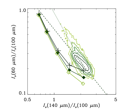
Figure 8: FIR colour-colour ($60~{}\mu{\rm m}-100~{}\mu{\rm m}$ vs. $140~{}\mu{\rm m}-100~{}\mu{\rm m}$) relation for various heat capacities. The other quantities adopted for calculations are the same as those in Figure 2. The filled squares represent the colour-colour relation with the heat capacity given in the text for graphite, and the crosses and open squares show the results with heat capacities multiplied by 1/2 and 2, respectively. The contours and the dashed and dotted lines are the same as those in Figure 2.

In our calculation, the optical constants from UV to FIR are required. The above materials have such data and are suitable for our work. For completeness, we should examine all kinds of possible species, but this is obviously impossible. However, the above robustness of the predicted FIR colour-colour relation implies that the detailed wavelength dependence of the optical constants is not reflected in the FIR colour-colour relation. We also note that the wavelength dependence in the FIR absorption efficiency (emissivity) is roughly proportional to $\lambda^{-2}$ (i.e. $\beta\simeq 2$) for all the above species. As shown in text, the FIR colour-colour relation is sensitive to the FIR emissivity index. A similar wavelength dependence of FIR emissivity is the reason why the above species produce similar FIR colour-colour relations.

A.2 Heat capacity

The difference in the heat capacity may affect the temperature of the VSGs. The LG temperature is not affected by the heat capacity since it is determined by the equilibrium temperature independent of the heat capacity (e.g. Draine & Lee, 1984). Thus, we expect that the difference in heat capacity may cause a variation of the 60 $\mu$m intensity. Here we test heat capacities whose values are 1/2 and 2 times of the value adopted in the text for graphite. The resulting colour-colour relations are shown in Figure 8. As expected above, the 140 $\mu$m–100 $\mu$m colour, which reflects the equilibrium temperature, is not affected by the change of heat capacity. This also supports our assumption that the contribution from VSGs is negligible at $\lambda\geq 100~{}\mu$m. The 60 $\mu$m–100 $\mu$m flux ratio becomes higher for smaller heat capacity, since the temperature of a VSG rises more when a photon is absorbed. At the same time, however, the grains rapidly cool if the heat capacity is small. Those two effects compensate, and the 60 $\mu$m–100 $\mu$m colour does not drastically change. Moreover, since the contribution from LGs in radiative equilibrium at the 60 $\mu$m band becomes larger for higher ISRF, the difference in the 60 $\mu$m–100 $\mu$m for $\chi\ga 3$ is negligible. Thus, we conclude that the change of grain heat capacity does not affect our results in the text.

Appendix B The Galactic Star Formation Rate

In section 5.2, we introduce the number of regions with young massive stars, $N_{\rm SF}$, to explain the fraction of sightlines associated with the sub-correlation. The number of such regions reflects the recent star formation activity of the Galaxy. Thus, we relate $N_{\rm SF}$ with the Galactic star formation rate (SFR).

We assume that the Galactic disk has a radius of $R_{\rm d}$ with thickness of $2H_{\rm d}$ (we assume $R_{\rm d}=10$ kpc and $H_{\rm d}=100$ pc). For simplicity, we assume that the regions with massive stars distribute uniformly in the Galactic plane. Then, $N_{\rm SF}$ can be estimated as $N_{\rm SF}/(\pi R_{\rm d}^{2}H_{\rm d})$.

The total UV luminosity in the entire galaxy can be estimated as $N_{\rm SF}\ell_{\rm UV}$, where $\ell_{\rm UV}$ is the UV luminosity of a region with massive stars. This can be converted to the SFR as (Inoue et al., 2000)

$${\rm SFR}=\frac{N_{\rm SF}\ell_{\rm UV}}{1.8\times 10^{9}~{}L_{\odot}}\,M_{\odot}~{}{\rm yr}^{-1}\,.$$ (26)

Since $\ell_{\rm UV}\simeq 2.8\times 10^{5}~{}L_{\odot}$, we obtain ${\rm SFR}=1.56\times 10^{-4}N_{\rm SF}~{}M_{\odot}~{}{\rm yr}^{-1}$.

The total luminosity of the Galactic OB stars is estimated to be $\sim 2.3\times 10^{9}~{}L_{\odot}$ (Mathis et al., 1983). Equating this with $N_{\rm SF}\ell_{\rm SF}$, we obtain $N_{\rm SF}\sim 8.2\times 10^{3}$ (or ${\rm SFR}=1.3~{}M_{\odot}$ yr^-1). If this number is used in equation (25), we obtain the probability that a line of sight is associated with a high radiation field of $\chi\sim 10$.

References

- Agladze et al. (1996) Agladze, N. I., Sievers, A. J., Jones, S. A., Burlitch, J. M., & Beckwith, S. V. W. 1996, ApJ, 462, 1026
- Aguirre et al. (2003) Aguirre, J. E., et al. 2003, ApJ, 596, 273
- Bianchi, Davies, & Alton (1999) Bianchi, S., Davies, J. I., & Alton, P. B. 1999, A&A, 344, L1
- Buat & Xu (1996) Buat, V., & Xu, C. 1996, A&A, 306, 61
- Bohlin, Savage, & Drake (1978) Bohlin, R. C., Savage, B. D., & Drake, J. F. 1978, ApJ, 224, 132
- Dasyra et al. (2005) Dasyra, K. M., Xilouris, E. M., Misiriotis, A., & Kylafis, N. D. 2005, A&A, 437, 447
- del Burgo et al. (2003) del Burgo, C., Laureijs, R. J., Ábrahám, P., & Kiss, Cs. 2003, MNRAS, 346, 403
- Désert, Boulanger, & Puget (1990) Désert, F.-X., Boulanger, F., & Puget, J. L. 1990, A&A, 237, 215
- Dobashi et al. (2005) Dobashi, K., Uehara, H., Kandori, R., Sakurai, T., Kaiden, M., Umemoto, T., & Sato, F. 2005, PASJ, 57, S1
- Dopita et al. (2005) Dopita, M. A., et al. 2005, ApJ, 619, 755
- Dorschner et al. (1995) Dorschner, J., Begemann, B., Henning, Th., Jäger, C., & Mutschke, H. 1995, A&A, 300, 503
- Draine & Anderson (1985) Draine, B. T., & Anderson, N. 1985, ApJ, 292, 494
- Draine & Lee (1984) Draine, B. T., & Lee, H. M. 1984, ApJ, 285, 89
- Draine & Li (2001) Draine, B. T., & Li, A. 2001, ApJ, 551, 807 (DL01)
- Draine & Li (2007) Draine, B. T., & Li, A. 2007, ApJ, 657, 810
- Dwek et al. (1997) Dwek, E., et al. 1997, ApJ, 475, 565
- Edo (1983) Edo, O. 1983, PhD Thesis, University of Arizona
- Fukui (2001) Fukui, Y., Mizuno, N., Yamaguchi, R., Mizuno, A., & Onishi, T. 2001, PASJ, 53, L41
- Guhathakurta & Draine (1989) Guhathakurta, P., & Draine, B. T. 1989, ApJ, 345, 230
- Hibi (2006) Hibi, Y. 2006, PhD Thesis, Nagoya University
- Hibi et al. (2006) Hibi, Y., Shibai, H., Kawada, M., Ootsubo, T., & Hirashita, H. 2006, PASJ, 58, 509
- Hildebrand (1983) Hildebrand, R. H. 1983, QJRAS, 24, 267
- Hirashita et al. (2003) Hirashita, H., Buat, V., & Inoue, A. K. 2003, A&A, 410, 83
- Hirashita & Ferrara (2002) Hirashita, H., & Ferrara, A. 2002, MNRAS, 337, 921
- Hirashita et al. (2001) Hirashita, H., Inoue, A. K., Kamaya, H., & Shibai, H. 2001, A&A, 366, 83
- Hirashita et al. (2005) Hirashita, H., Nozawa, T., Kozasa, T., Ishii, T. T., & Takeuchi, T. T. 2005, MNRAS, 357, 1077
- Huffman & Stapp (1973) Huffman, D. R., & Stapp, J. L. 1973, in Greenberg J. M., van de Hulst H. C., eds., IAU Symp. Vol. 52, Interstellar Dust and Related Topics, Reidel, Dordrecht, p. 297
- Iglesias-Páramo et al. (2004) Iglesias-Páramo, J., Buat, V., Donas, J., Boselli, A., & Milliard, B. 2004, A&A, 419, 109
- Inoue et al. (2000) Inoue, A. K., Hirashita, H., & Kamaya, H. 2000, PASJ, 52, 539
- Jones (2000) Jones, A. P. 2000, J. Geophys. Res., 105, 10257
- Jones et al. (1996) Jones, A. P., Tielens, A. G. G. M., & Hollenbach, D. J. 1996, ApJ, 469, 740
- Kennicutt (1998) Kennicutt, R. C., Jr. 1998, ARA&A, 36, 189
- Kiuchi et al. (2004) Kiuchi, G., Ohta, K., Sawicki, M., & Allen, M. 2004, AJ, 128, 2743
- Lagache et al. (1998) Lagache, G., Abergel, A., Boulanger, F., & Puget, J.-L. 1998, A&A, 333, 709
- Li & Draine (2001) Li, A., & Draine, B. T. 2001, ApJ, 554, 778
- Li & Greenberg (1997) Li, A., & Greenberg, J. M. 1997, A&A, 323, 566
- Li, Misselt, & Wang (2006) Li, A., Misselt, K. A., & Wang, Y. J. 2006, ApJ, 640, L151
- Mathis (1990) Mathis, J. S. 1990, ARA&A, 28, 37
- Mathis et al. (1983) Mathis, J. S., Mezger, P. G., & Panagia, N. 1983, A&A, 128, 212
- Mathis et al. (1977) Mathis, J. S., Rumpl, W., & Nordsieck, K. H. 1977, ApJ, 217, 425
- Matsuhara et al. (2006) Matsuhara, H., et al. 2006, PASJ, 58, 673
- Murakami (2004) Murakami, H. 2004, Proc. SPIE, 5487, 330
- Nagata et al. (2002) Nagata, H., Shibai, H., Takeuchi, T. T., & Onaka, T. 2002, PASJ, 54, 695
- Onaka et al. (2007) Onaka, T., Tokura, D., Sakon, I., Tajiri, Y. Y., Takagi, T., & Shibai, H. 2007, ApJ, 654, 844
- Pei (1992) Pei, Y. C 1992, ApJ, 395, 130
- Okada et al. (2006) Okada, Y., Onaka, T., Nakagawa, T., Shibai, H., Tomono, D., & Yui, Y. Y. 2006, ApJ, 640, 383
- Reach et al. (1995) Reach, W. T., et al. 1995, ApJ, 451, 188
- Sakon et al. (2004) Sakon, I., Onaka, T., Ishihara, D., Ootsubo, T., Yamamura, I., Tanabé, T., & Roellig, T. L. 2004, ApJ, 609, 203
- Sakon et al. (2007) Sakon, I., et al. 2007, ApJ, 651, 174
- Shibai (2004) Shibai, H. 2004, Advances in Space Research, 34, 589
- Smith et al. (1978) Smith, L. F., Biermann, P., & Mezger, P. G. 1978, A&A, 66, 65
- Stevens, Amure, & Gear (2005) Stevens, J. A., Amure, M., & Gear, W. K. 2005, MNRAS, 357, 361
- Takagi et al. (2003) Takagi, T., Vansevičius, V., & Arimoto, N. 2003, PASJ, 55, 385
- Takeuchi et al. (2003) Takeuchi, T. T., Hirashita, H., Ishii, T. T., Hunt, L. K., & Ferrara, A. 2003, MNRAS, 343, 839
- Takeuchi et al. (2005) Takeuchi, T. T., Ishii, T. T., Nozawa, T., Kozasa, T., & Hirashita, H. 2005, MNRAS, 362, 592
- Tumlinson et al. (2002) Tumlinson, J., et al. 2002, ApJ, 566, 857
- Weingartner & Draine (2001) Weingartner, J. C., & Draine, B. T. 2001, ApJ, 548, 296
- Welty et al. (2001) Welty, E. W., Lauroesch, J. T., Blades, J. C., Hobbs, L. M., & York, D. G. 2001, ApJ, 554, L75
- Werner et al. (2004) Werner, M. W., et al. 2004, ApJS, 154, 1
- Wright et al. (1991) Wright, E. L., et al. 1991, ApJ, 381, 200