The structure of the Galactic halo: SDSS versus SuperCOSMOS

Abstract

The halo structure at high Galactic latitudes near both the north and south poles is studied using SDSS and SuperCOSMOS data. For the south cap halo, the archive of the SuperCOSMOS photographic photometry sky survey is used. The coincident source rate between SuperCOSMOS data in $B_{J}$ band from $16^{m}.5$ to $20^{m}.5$ and SDSS data is about 92%, in a common sky area in the south. While that in the $R_{F}$ band is about 85% from $16^{m}.5$ to $19^{m}.5$. Transformed to the SuperCOSMOS system and downgraded to the limiting magnitudes of SuperCOSMOS, the star counts in the northern Galactic cap from SDSS show up to an $16.9\pm 6.3\%$ asymmetric ratio (defined as relative fluctuations over the rotational symmetry structure) in the $B_{J}$ band, and up to $13.5\pm 6.7\%$ asymmetric ratio in the $R_{F}$ band. From SuperCOSMOS $B_{J}$ and $R_{F}$ bands, the structure of the southern Galactic hemisphere does not show the same obvious asymmetric structures as the northern sky does in both the original and downgraded SDSS star counts. An axisymmetric halo model with n=2.8 and q=0.7 can fit the projected number density from SuperCOSMOS fairly well, with an average error of about 9.17%. By careful analysis of the difference of star counts between the downgraded SDSS northern halo data and SuperCOSMOS southern halo data, it is shown that no asymmetry can be detected in the south Galactic cap at the accuracy of SuperCOSMOS, and the Virgo overdensity is likely a foreign component in the Galactic halo.

1 Introduction

The modern use of star counts in the study Galatic structure began with Bahcall & Soneira (1980). In Bahcall’s standard model, the structure of the Galaxy is assumed to be an exponential disk and a de Vaucouleurs spheriodal halo. A lot of work has been done to constrain and examine this theoretical model, as summarised in Xu, Deng & Hu (2006) (XDH06 here after), most of them using only a small sky area. The global structure of the Galactic halo can only be inferred by different observations of small sky areas with different magnitude limits, photometric passbands and different original observational goals. SDSS provides us with the opportunity to examine the large scale structure of the Galaxy from optical photometry thanks to its deep photometry and large sky coverage. From SDSS observational data it is clear that the stellar halo of the Galaxy is aymmetric, contrary to what has been generally assumed. From colour star counts it is obvious that the asymmetric projected stellar number density is produced by halo stars. There are two possible explanations for such a halo structure. Firstly, that there are some large scale star streams embedded in the axi-symmetric smooth structure of the Galactic halo (Jurić et al. 2005). Secondly, that the galactic stellar halo is intrinsically not axi-symmetric (Newberg & Yanny 2005; XDH 2006). Based on the data we have so far, some combination of the two might also be possible . In Paper I, we tested the second option and fitted the observational data with triaxial halo. The triaxial halo model fits fairly well the projected number density near the northern cap of the Galactic stellar halo. However, in some sky areas, the triaxial halo model cannot reproduce the actual star counts. The multi-solutions that are intrinsic in fitting the observational data with the triaxial halo model make the interpretation of the data somewhat difficult. On the other hand, the alternative option where the asymmetry of the halo is caused by large scale star streams also has some problems, even if the overwhelmingly large Virgo overdensity that covers nearly a quarter of the northern hemisphere can be explained by a large scale star stream. The observed underdensity near Ursa Major with respect to the assumed axi-symmetric halo still challenges such a picture. Nevertheless, the conservation of such a huge structure in the gravitational well of the Galaxy certainly needs to be verified. Martínez-Delgado et al. (2006) show that the Virgo overdensity can be reproduced by the dynamical evolution of the Sgr stream. Assuming a certain structure of the stellar halo (an oblate ellipse), their numerical simulation can predict an overdensity on a few hundred square degree scale.

Although it is the most advanced photometric sky survey in terms of depth and data quality, SDSS does not have good data coverage near the southern cap of the Galaxy which is, of course, crucial in understanding the overall structure of the stellar halo. Limited to the sky coverage of SDSS photometry database, it is probably premature to draw a firm conclusion on the stellar halo structure. Assuming that the Galactic stellar halo is non axi-symmetric, and can be described by a triaxial model, there must be some corresponding evidence in the southern hemisphere similar to what is found in XDH06 for the northern cap. In the axisymmetric halo model, the maximum star counts should be at longitude $l=0^{\circ}$ (due to the location of the observer). In the case of a triaxial halo, however, the maximum projected number density also depends on a certain parameters of the halo including azimuth angle, axial ratios and the limiting magnitudes of the observations. In the simplest case, the plane defined by the primary and the middle axis of the triaxial halo stays in the Galactic disk, the azimuth angle is only related with the angle between the primary axis and the direction of the Galactic center from the Sun, therefore the expected star counts and asymmetric ratio of northern and southern sky ought to be mirror symmetric with respect to the Galactic plane, i.e. what was found in the north cap should also be found in the south under such a halo model. If the two planes do not overlap, the situation will be more complicated, but similar results should still hold.

It is also interesting to examine archived sky survey data that has the good coverage and reasonable quality in the southern Galactic halo: the photographic photometry of SuperCOSMOS is ideal for this purpose. As reviewed by Hambly et al. (2001a), photographic observations for the Galaxy started in the late nineteenth century. In the 1930s, the development of Schmidt telescopes with wide fields of view further advanced photographic surveys. The 1.2-m Palomar Oschin, 1.0-m ESO and 1.2-m UK Schmidt telescopes finished the photographic whole sky survey in the last century, such surveys form a legacy library for examining the structure of the Galaxy. In the late twentieth century, the photographic plates were eventually digitized using microdensitometry and digital electronics machines. There are several major programs to digitize the photographic plates, of which SuperCOSMOS is one. In Hambly et al. (2001a), a general overview of these programmes (APM, APS, COSMOS, DSS, PMM, SuperCOSMOS) is presented. The digitized photographic sky survey of SuperCOSMOS provides a catalog of three bands, namely blue($B_{J}$), red($R_{F}$) and near-infrared($I_{VN}$), which have deeper detection limit for the same detection completeness compared to other similar survey programs (see fig2 of Hambly et al. 2001a). We therefore adopt the SuperCOSMOS data archive for our present study.

In section 2, the observational data are described and the stellar source cross identification between the SuperCOSMOS data and the SDSS data is carried out, and the viability of using SuperCOSMOS data to study the structure of southern Galactic stellar halo is discussed. In section 3,downgraded SDSS and SuperCOSMOS observational of star counts results are presented. In section 4, the model fits to the SuperCOSMOS star counts are introduced. In section 5, the SuperCOSMOS observational data and theoretical models are compared, and SuperCOSMOS southern sky star counts and SDSS downgraded northern sky star counts also compared and analyzed. In section 6, the result of star counts is summarized.

2 The observational data

2.1 SuperCOSMOS photometric data

The SuperCOSMOS Sky Survey is a digitized photography sky survey. It is described in detail in a series of papers by Hambly and collaborators (Hambly et al. 2001a; Hambly, Irwin & MacGillivray 2001b; Hambly, Davenhall & Irwin 2001c).

The SuperCOSMOS photography atlas of the SuperCOSMOS sky survey includes blue($B_{J}$), red($R_{F}$), and near infrared($I_{VN}$) passband photometric survies carried out by UK Schmidt survey for $-90^{\circ}<Dec<+2.5^{\circ}$, ESO Red Survey of $-90^{\circ}<Dec<-17.5^{\circ}$, and Palomar surveies including, POSS-I Red Survey for $-20.5^{\circ}<Dec<+2.5^{\circ}$, POSS-II Blue Survey for $-2.5^{\circ}<Dec<+90.0^{\circ}$, POSS-II Red Survey for $-2.5^{\circ}<Dec<+90.0^{\circ}$. Data of $B_{J}$ band has 90% or about detection completeness from $16^{m}.5$ to $20^{m}.5$, and that of $R_{F}$ band has same completeness from $16^{m}.5$ to $19^{m}.5$ mag. The photometric data has a magnitude error of $0^{m}.3$, but color is accurate to about $0^{m}.16$(Hambly et al. 2001a).

There are two interface applications of SuperCOSMOS: the SuperCOSMOS Sky Survey (http:// www-wfau.roe.ac.uk/sss, SSS hereafter) and the SuperCOSMOS Sky Archive (http:// surveys.roe.ac.uk/ssa, SSA hereafter).

Images of small sky areas and catalogs from the SuperCOSMOS sky survey can be downloaded. We thank the SuperCOSMOS working group who made all the data available to the community. The SSA only includes photometric data from UKST and ESO. As made clear by Hambly et al.(2001a), although the entire sky is digitized, the data in this archive is released progressively. The total amount of data is enormous, only F type stars (selected by 0.504 $\leq B_{J}-R_{F}\leq$ 0.8236 ) from $20^{m}.4$ to $20^{m}.415$ are adopted to show the sky coverage which is in the upper panel of figure 1. The survey covers most of the high latitude southern sky, and a little of the northern hemisphere. The clump at (l,b)=($302.616^{\circ},-44.580^{\circ}$) is the SMC, and the clump at (l,b)=($280.085^{\circ},-30.430^{\circ}$) is the LMC.

Except for the difference in sky coverage, the two interface applications use different selection standards. The SSA SQL selection is much more configurable (private communication by email with Hambly) than that of the SSS. For example, there are 4 kinds of B magnitude in the SSA, namely classMagB (B band magnitude selected by B image class), gCorMagB (B band magnitude assuming the object is a galaxy), sCorMagB(B band magnitude assuming the object is a star), classB (image classification from B band detection). The most appropriate attribute for point sources is sCorMag, while the most possible class of an object from all three bands is provided by parameter “meanclass”. The SSS only includes selection parameters applied to the primary passband, coresponding to classB of the SSA in the example. Our aim is to count the stars in each selected sky area, and using classB will lose some stars due to not synthesizing information of all the three bands. This will influence the result of star counts seriously. So “sCorMagB” of the SSA data is selected to carry out the study and the “meanclass” is limited to 2(star label). Because the SSA only covers limited sky areas of high latitude northern galactic hemisphere (upper panel of figure 1) we cannot directly compare SuperCOSMOS star counts of northern sky with those of SDSS.

The SSA includes $R_{F}$ band data from both UKST and ESO. However data from the $R_{F}$ band of UKST is deeper than that of ESO. Therefore, only UKST is adopted. The detailed instrumental specifications of UKST can be found in Cannon (1984), the main parameters of the survey telescope and instruments are listed in table 1.

Table 1: Parameters of telescope of UKST

site	Siding Spring Mountain, -31∘S
aperture	1.24m
focal, focal ratio	3.07m, f/2.5
photographic plates	Kodak IIIa-J emulsion, 356$mm^{2}$, 67.1 arcsec $mm^{-1}$, 6.5${}^{\circ}\times$6.5∘
primary pointing accuracy	$\pm$6 arcsec r.m.s.

As demonstrated in the upper panel of figure 1, the UKST atlas of SuperCOSMOS covers most of the high Galactic latitude southern hemisphere. The structure of the Galactic halo near the southern cap can be studied using a stellar photometry catalog selected in a similar way as we did for the northern sky in XDH06, shown here in the lower panel of Fig 1. The selected sky area for this work is shown in lower panel of figure 1, the Lambert projection of southern hemisphere. Each of the squares represents a rectangular sky area of about $2^{\circ}\times 2^{\circ}$. Some of the selected sky areas may be trimmed if sitting near the survey’s edge, or the region is masked by contaminats such as saturated bright stars, or clumps such as the dwarf galaxy IC1613 in ($130^{\circ},-60^{\circ}$). The first group of sky areas are along a circle of $b=-60^{\circ}$, equally spaced by $10^{\circ}$. The other 12 groups are a selection of sky areas along longitudinal directions equally spaced by $30^{\circ}$. At a given longitude, the sky areas are selected by a step of $5^{\circ}$. This selection of sky areas can evenly cover the southern Galactic cap, so that the global structure of the halo near the southern pole can be examined.

2.2 Cross checking of SuperCOSMOS and SDSS data sets

In our previous work (XDH06), SDSS data is used to study the structure of the Galactic stellar halo near the Northern Galactic pole, The SDSS catalog providing a uniform and accurate photometric data set. The five broadband filters, u,g,r,i,z are 95% complete to $22^{m}.0,22^{m}.2,22^{m}.2,21^{m}.3,20^{m}.5$ respectively, and the uncertainty in the photometry is about 3% at g=$19^{m}$(Chen et al. 2001).

Compared to the high-quality photometry data of SDSS, the SuperCOSMOS data has a narrower dynamic range, lower magnitude limit and larger photometric error, due to photographic photometry. To evaluate any uncertainties due to misclassifications and the relatively less accurate photometry of SuperCOMOS, a comparison in areas common to both surveys is needed.

The photometric calibration between SDSS and SuperCOSMOS has been made available by the 2dF Galaxy Redshift Survey(2DFGRS) Final Data Release Photometric Calibration which defines a set of color equations in its final data . The $B_{J}$ band is correlated with SDSS g and r band, $B_{J}=0.15+0.13\times(g-r)$, while $R_{F}$ is very similar to SDSS r band, $R_{F}$=r-0.13. The results of such color calibration are shown in figure 2 .

The two small sky areas with superpositions of SDSS and SuperCOSMOS surveys in both the northern and southern sky are chosen to examine the color equations and the classification of SuperCOSMOS objects. The northern area is located at ($l,b$)=($280^{\circ},60^{\circ}$) with $2^{\circ}\times 2^{\circ}$ field of view (FOV), the southern area is at ($l,b$)=($62^{\circ},-59^{\circ}$) with $1^{\circ}\times 4^{\circ}$ FOV. The equinox of SuperCOSMOS data associated with the photometric image library is J2000.0. The position accuracy of SuperCOSMOS is $\pm$0.2arcsec at $B_{J}=19^{m}$,$R_{F}=18^{m}$, $\pm$0.3arcsec at $B_{J}=22^{m}$,$R_{F}=21^{m}$ (Hambly et al 2001c). Taking into account proper motion, cross-identification is carried out between SDSS and SuperCOSMOS in the two superimposed sky areas in a identification criterion box of $0^{m}.3$ and 10 arcsec. In such a box, multiple sources can be present, the pair of stars with the nearest coordinates and magnitudes are identified as the same source. We take the SDSS data as the “true” values of both position and magnitude. Based on the matched star list in the two areas, uncertainties in the magnitude of SuperCOSMOS photometry for each object can be measured. The systematic error calculated this way infers the error of the color equations from 2DFGRS calibration; while the scatter can be used to measure the error in SuperCOSMOS photometric data. Fitting the systematic error with a 2nd order polynomial, the color equations are refined. Using the modified color equations, $B_{J}$ and $R_{F}$ magnitude of SDSS data is defined as $B_{JSDSS}$=g+0.15+0.13$\times$(g-r)+ $\bigtriangleup{mod}$, $R_{FSDSS}$=r-0.13+$\bigtriangleup{mod}$. Iterating the cross-identification procedure reduces the systematic error. The error in the SuperCOSMOS data in the $B_{J}$ band is found to be $\epsilon_{B_{J}}$ = $B_{J}$ - $B_{JSDSS}$, and that in $R_{F}$ $\epsilon_{R_{J}}$ = $R_{F}$ - $R_{FSDSS}$. The variance of the errors as functions of magnitude is obtained from fitting the scatter with a gaussian.

After such modification, and repeating the cross-identification, the source matching ratios between the two surveys are improved. In the end, the SuperCOSMOS data matches that of SDSS in the $B_{J}$ band magnitude limits by 92-93% in a 10 arcsec and $0^{m}.3$ box. For the $R_{F}$ band, the matching ratio can be raised to 85% or larger in the $16^{m}.5-19^{m}.5$ magnitude range. The matching ratio of the $R_{F}$ band is not as good as that of the $B_{J}$ band, this is likely due to the lower sensitivity in the $R_{F}$ band. A 85% is still lower than the intrinsic completeness estimated for different surveys in the SuperCOSMOS atlas (see figure 12b of Hambly et al. 2001b). This is possibly caused by the brighter magnitude limit of the SSA compared to that of SDSS as the bright stars are saturated, therefore influencin more neighbours.

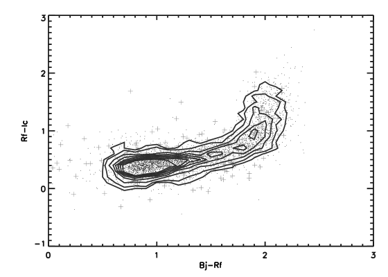
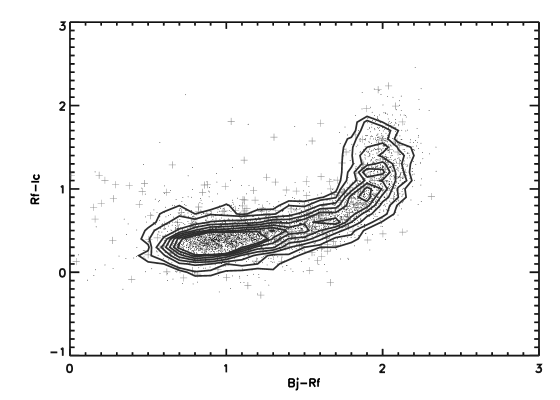
Figure 3: The cross identification between the SuperCOSMOS and SDSS data sets in color-color space. The contour and the black points on the color-color diagram represent the $B_{J}$ band matched sources in the same overlapping sky areas, limited in $0^{m}.3$ in magnitude and 10 arcsec in angular distance box and a magnitude interval of $16^{m}.5<B_{J},B_{JSDSS}<20^{m}.5$. The crosses represent the unmatched sources. The upper panel: The northern overlapped sky area around $(280^{\circ},60^{\circ})$; The lower panel: the southern one around $(62^{\circ},-59^{\circ})$.

In the upper and lower panel of figures 3, the contours in the color-color diagram represent the SuperCOSMOS data in the three bands that are cross-identified in the SDSS data. Black points over-plotted on the contours are the matched stellar sources, while the crosses represent SuperCOSMOS sources which are unmatched.

3 Observational star counts

3.1 Star counts from downgraded SDSS data

The examination of halo structure through star counts depends critically on the depth of the photometry. The SSA has a narrower dynamic range and shallower detection limit than SDSS. A test is carried out to check if the asymmetric structure found in XDH06 is still present with the shallower limit of SSA data. The data used in XDH06 is downgraded by applying the SuperCOSMOS magnitude limits, photometric errors of SuperCOSMOS are also added to the SDSS data. A Monte-Carlo method is used to reproduce the photometric errors as of SuperCOSMOS $\epsilon_{B_{J}}$, $\epsilon_{R_{F}}$ (Rockosi private communication). Gaussian errors similar in size to those of the SuperCOSMOS data are added to the magnitude of each star before measuring the star counts. We find that the results of XDN06 are recovered, with the average fluctuation raised only by about 3.7%. After transforming into the SuperCOSMOS system, the errors are $16^{m}.5<B_{JSDSS}<20^{m}.5$ and $16^{m}.5<R_{FSDSS}<19^{m}.5$ respectively.

Figure 4 and Figure 5 show the star counts from the SDSS data with same sky areas as in XDH06 but downgraded to the SuperCOSMOS magnitude limits, for $B_{JSDSS}$ and $R_{FSDSS}$ respectively. From the present SDSS public data release, the sky area $l=210^{\circ}$ is now added. Panel a) is for star counts in sky areas along the $b=60^{\circ}$ circle. Panels b)-f) are for star counts of sky areas along the selected longitudinal directions paired by mirror symmetry on the both sides of the $l=0^{\circ}$ meridian. The asymmetric structure still appears clearly with the magnitude limit of the downgraded SDSS data (especially in figure 4a). The asymmetric structure is not so prominent as with the original SDSS magnitude limits, but we can still see that the star counts in $l\in[180^{\circ},360^{\circ}]$ are systematically higher than in $l\in[0^{\circ},180^{\circ}]$. The largest asymmetry of star counts appear in panels b), c) and d). In panels e) and f), the errors are so large at the downgraded limits that the asymmetric differences between sky areas found in XDH06 are only marginally visible. As in figure 4, figure 5 shows the results of star counts from the $R_{FSDSS}$ data. Again, the most prominent excess over mirror symmetry is found in panels b), c) and d). However, the $R_{FSDSS}$ band magnitude limit is fainter than that of the $B_{JSDSS}$ band, which leads to weaker features of asymmetry than figure 4. Tables 2 and 3 describe the asymmetric ratio and its uncertainty in the downgraded SDSS data. Columns 1–4 are the Galactic coordinates ($l$ and $b$), counted numbers and the corresponding errors for sky areas with $l\leq 180^{\circ}$, and columns 5–8 are the same quantities for sky areas on the other side of the $l=0^{\circ}$ meridian. Comparison is between sky areas paired with mirror symmetry with respect to the $l=0^{\circ}$ meridian. The asymmetric ratios are defined by: $asymmetric\>ratio=(number\>density_{2}-number\>density_{1})/(number\>density_{1})\times 100\%$ which are given in column 9; column 10 gives the uncertainties in the ratios which are inferred from the error of the number densities (tables 4–5 all have the same entries, but for different data). The asymmetric ratios measured from downgraded SDSS data are all positive with one exception which is very near to zero, this means that all the sky areas in $l\in[180^{\circ},360^{\circ}]$ have higher projected number densities than those in $l\in[0^{\circ},180^{\circ}]$. The largest asymmetric ratio is $16.9\pm 6.3\%$ in the $B_{JSDSS}$ band and $13.5\pm 6.7\%$ in the $R_{FSDSS}$ band.

Therefore if there are similar levels of asymmetric structure in the southern Sky, they should be visible even with the SuperCOSMOS magnitude limit.

Table 2: The relative deviations of the sky field pairs for $B_{JSDSS}$$\in[16^{m}.5,20^{m}.5]$ mag.

$\ell_{1}$	$b$	number	error of	$\ell_{2}$	$b$	number	error of	asymmetry ratio	uncertainty of
$(^{\circ})$	$(^{\circ})$	$density_{1}$	$density_{2}$	$(^{\circ})$	$(^{\circ})$	$density_{1}$	$density_{2}$	($\%$)	asymmetry ratio ($\%$)
10	60	1597.500	48.330	350	60	1685.949	21.825	5.536	4.391
40	60	1389.890	13.915	320	60	1595.569	19.651	14.798	2.415
50	60	1420.219	75.928	310	60	1581.060	38.915	11.325	8.086
60	60	1377.050	38.606	300	60	1387.020	74.542	0.724	8.216
70	60	1258.550	31.836	290	60	1428.900	61.433	13.535	7.410
80	60	1124.489	49.622	280	60	1283.959	42.167	14.181	8.162
90	60	1081.709	44.143	270	60	1264.489	24.530	16.897	6.348
100	60	1074.750	56.961	260	60	1133.510	11.626	5.467	6.381
110	60	1010.599	31.438	250	60	1049.510	16.462	3.850	4.739
120	60	961.590	4.174	240	60	1056.290	37.484	9.848	4.332
130	60	908.416	44.612	230	60	989.323	39.663	8.906	9.277
150	60	870.270	41.345	210	60	911.882	17.599	4.781	6.773
170	60	866.552	30.676	190	60	871.720	34.395	0.596	7.509
30	65	1303.510	60.955	330	65	1476.130	50.739	13.242	8.568
30	70	1219.079	24.728	330	70	1266.099	43.532	3.857	5.599
30	75	1101.650	38.571	330	75	1146.250	13.678	4.048	4.742
60	65	1195.140	37.210	300	65	1326.010	35.114	10.950	6.051
60	70	1110.910	14.796	300	70	1220.300	42.086	9.846	5.120
60	75	1005.109	33.589	300	75	1100.689	58.191	9.509	9.131
90	55	1229.219	54.959	270	55	1347.400	30.259	9.614	6.932
90	65	1023.700	26.978	270	65	1166.369	56.959	13.936	8.199
90	70	955.830	39.693	270	70	1098.619	18.859	14.938	6.125
90	75	913.866	15.131	270	75	1017.349	31.349	11.323	5.086
120	55	1028.329	28.122	240	55	1090.479	54.862	6.043	8.069
120	65	919.445	50.675	240	65	991.031	56.564	7.785	11.663
150	65	828.664	24.510	210	65	901.859	33.080	8.832	6.949
150	70	806.091	18.853	210	70	841.559	19.937	4.399	4.812
150	75	837.734	51.541	210	75	851.314	22.645	1.621	8.855

Table 3: The relative deviations of the sky field pairs for $R_{FSDSS}$$\in[16^{m}.5,19^{m}.5]$ mag.

$\ell_{1}$	$b$	number	error of	$\ell_{2}$	$b$	number	error of	asymmetry ratio	uncertainty of
$(^{\circ})$	$(^{\circ})$	$density_{1}$	$density_{1}$	$(^{\circ})$	$(^{\circ})$	$density_{2}$	$density_{2}$	($\%$)	asymmetry ratio ($\%$)
10	60	1726.890	50.382	350	60	1811.989	31.156	4.927	4.721
40	60	1544.520	17.300	320	60	1730.890	27.820	12.066	2.921
50	60	1549.510	97.815	310	60	1695.439	58.618	9.417	10.095
60	60	1458.390	25.113	300	60	1493.660	75.721	2.418	6.914
70	60	1338.709	40.464	290	60	1508.959	52.391	12.717	6.936
80	60	1246.390	55.123	280	60	1374.219	37.407	10.256	7.423
90	60	1174.689	54.628	270	60	1333.349	23.945	13.506	6.688
100	60	1155.189	66.160	260	60	1209.199	9.641	4.675	6.561
110	60	1103.040	32.209	250	60	1141.750	19.037	3.509	4.645
120	60	1043.449	30.933	240	60	1138.829	34.655	9.140	6.285
130	60	985.525	19.785	230	60	1043.609	65.759	5.893	8.680
150	60	947.528	54.534	210	60	973.794	15.702	2.772	7.412
170	60	950.013	29.894	190	60	954.971	48.084	0.521	8.208
30	65	1425.650	58.515	330	65	1575.650	49.862	10.521	7.601
30	70	1322.020	12.712	330	70	1377.750	30.668	4.215	3.281
30	75	1186.050	34.852	330	75	1217.760	13.473	2.673	4.074
60	65	1291.579	29.649	300	65	1402.810	40.511	8.611	5.432
60	70	1214.660	22.258	300	70	1290.349	36.804	6.231	4.862
60	75	1094.579	24.285	300	75	1161.560	32.224	6.119	5.162
90	55	1359.380	48.864	270	55	1461.239	52.372	7.493	7.447
90	65	1093.819	37.443	270	65	1207.569	59.053	10.399	8.822
90	70	1036.369	20.023	270	70	1167.410	20.154	12.644	3.876
90	75	1006.340	4.486	270	75	1076.699	15.964	6.991	2.032
120	55	1124.869	42.921	240	55	1236.449	23.534	9.919	5.907
120	65	979.656	34.514	240	65	1067.819	57.995	8.999	9.443
150	65	893.812	35.045	210	65	959.431	42.456	7.341	8.670
150	70	867.317	21.781	210	70	895.692	25.912	3.271	5.498
150	75	919.247	32.209	210	75	917.749	21.114	-0.163	5.800

Table 4: The relative deviations of the sky field pairs for $B_{J}$$\in[16^{m}.5,20^{m}.5]$ mag.

$\ell_{1}$	$b$	number	error of	$\ell_{2}$	$b$	number	error of	asymmetry ratio	uncertainty of
$(^{\circ})$	$(^{\circ})$	$density_{1}$	$density_{1}$	$(^{\circ})$	$(^{\circ})$	$density_{2}$	$density_{2}$	($\%$)	asymmetry ratio ($\%$)
10	-60	1552.579	76.917	350	-60	1584.079	61.902	2.028	8.941
20	-60	1544.079	44.300	340	-60	1439.569	47.212	-6.768	5.926
30	-60	1515.079	66.156	330	-60	1409.569	58.819	-6.963	8.248
40	-60	1523.579	43.333	320	-60	1453.579	80.638	-4.594	8.136
50	-60	1422.069	63.642	310	-60	1380.069	53.733	-2.953	8.253
60	-60	1370.569	33.600	300	-60	1307.069	46.027	-4.633	5.809
70	-60	1179.930	27.163	290	-60	1351.569	71.606	14.546	8.370
80	-60	1132.560	49.012	280	-60	1247.060	87.287	10.109	12.034
90	-60	1053.050	34.337	270	-60	1191.060	31.689	13.105	6.270
100	-60	1006.549	66.823	260	-60	1089.060	41.794	8.197	10.791
110	-60	876.658	50.321	250	-60	1051.550	43.258	19.949	10.674
120	-60	938.547	57.981	240	-60	967.549	65.758	3.090	13.184
130	-60	905.307	43.079	230	-60	916.546	34.188	1.241	8.534
140	-60	895.546	34.853	220	-60	948.549	47.782	5.918	9.227
150	-60	859.044	34.550	210	-60	940.049	18.947	9.429	6.227
160	-60	919.547	18.449	200	-60	908.546	64.258	-1.196	8.994
170	-60	933.547	57.718	190	-60	838.543	32.895	-10.176	9.706
30	-55	1756.609	62.784	330	-55	1732.640	34.151	-1.364	5.518
30	-65	1336.380	25.611	330	-65	1302.069	36.909	-2.567	4.678
30	-70	1190.050	115.05	330	-70	1225.869	55.002	3.009	14.289
30	-75	978.531	76.464	330	-75	1014.270	20.205	3.652	9.879
30	-80	904.171	96.671	330	-80	1026.550	49.882	13.534	16.208
60	-55	1443.650	54.077	300	-55	1470.670	46.232	1.871	6.948
60	-65	1205.050	68.259	300	-65	1147.079	28.443	-4.810	8.024
60	-70	1079.670	37.970	300	-70	976.601	28.756	-9.546	6.180
60	-75	1093.479	42.780	300	-75	1015.239	50.576	-7.155	8.537
60	-80	918.567	53.861	300	-80	1048.150	164.492	14.106	23.771
90	-65	1057.750	37.072	270	-65	992.672	48.298	-6.152	8.070
90	-70	983.179	49.343	270	-70	950.286	28.261	-3.345	7.893
90	-75	985.293	81.426	270	-75	903.184	56.136	-8.333	13.961
90	-80	1002.070	76.915	270	-80	928.646	60.223	-7.327	13.685
120	-65	858.383	62.833	240	-65	929.966	73.010	8.339	15.825
120	-70	859.643	48.598	240	-70	921.046	57.155	7.142	12.302
120	-75	881.934	33.591	240	-75	925.401	15.142	4.928	5.525
120	-80	894.091	32.333	240	-80	833.622	57.494	-6.763	10.046
150	-65	885.005	24.511	210	-65	909.851	44.259	2.807	7.770
150	-70	836.981	64.097	210	-70	828.940	44.485	-0.960	12.973
150	-75	906.083	72.184	210	-75	835.567	49.243	-7.782	13.401
150	-80	810.585	25.940	210	-80	814.905	49.143	0.532	9.262

Table 5: The relative deviations of the sky field pairs for $R_{F}$$\in[16^{m}.5,19^{m}.5]$ mag.

$\ell_{1}$	$b$	number	error of	$\ell_{2}$	$b$	number	error of	asymmetry ratio	uncertainty of
$(^{\circ})$	$(^{\circ})$	$density_{1}$	$density_{1}$	$(^{\circ})$	$(^{\circ})$	$density_{2}$	$density_{2}$	($\%$)	asymmetry ratio ($\%$)
10	-60	1746.089	71.268	350	-60	1848.599	110.406	5.870	10.404
20	-60	1751.089	29.558	340	-60	1617.079	68.217	-7.652	5.583
30	-60	1761.089	91.829	330	-60	1644.089	143.147	-6.643	13.342
40	-60	1802.089	55.405	320	-60	1663.089	61.489	-7.713	6.486
50	-60	1693.589	96.918	310	-60	1591.079	23.517	-6.052	7.111
60	-60	1562.079	49.526	300	-60	1523.079	91.257	-2.496	9.012
70	-60	1444.229	42.711	290	-60	1539.579	80.699	6.602	8.545
80	-60	1335.069	58.455	280	-60	1432.069	93.267	7.265	11.364
90	-60	1217.560	39.018	270	-60	1472.579	46.217	20.945	7.000
100	-60	1176.060	49.969	260	-60	1348.569	69.336	14.668	10.144
110	-60	911.591	39.793	250	-60	1270.069	55.966	39.324	10.504
120	-60	1188.680	81.417	240	-60	1152.560	83.339	-3.038	13.860
130	-60	1133.849	59.553	230	-60	1070.560	23.034	-5.581	7.283
140	-60	1096.560	36.696	220	-60	1176.060	72.195	7.249	9.930
150	-60	997.552	66.039	210	-60	1140.560	34.719	14.335	10.100
160	-60	1146.060	46.602	200	-60	1115.060	166.630	-2.704	18.605
170	-60	1155.560	35.725	190	-60	1058.050	25.871	-8.438	5.330
30	-55	1959.729	64.605	330	-55	1961.910	30.947	0.111	4.875
30	-65	1537.520	61.215	330	-65	1549.349	41.863	0.769	6.704
30	-70	1509.489	116.808	330	-70	1416.660	114.977	-6.149	15.355
30	-75	1197.810	52.558	330	-75	1249.969	10.672	4.354	5.278
30	-80	1121.569	67.932	330	-80	1216.599	87.526	8.472	13.860
60	-55	1693.839	63.233	300	-55	1695.589	38.849	0.103	6.026
60	-65	1524.510	43.793	300	-65	1363.000	41.841	-10.594	5.617
60	-70	1308.469	62.136	300	-70	1183.469	24.054	-9.553	6.587
60	-75	1321.449	30.234	300	-75	1273.150	41.728	-3.655	5.445
60	-80	1151.810	68.150	300	-80	1254.030	125.622	8.874	16.823
90	-65	1262.430	45.872	270	-65	1193.810	57.514	-5.435	8.189
90	-70	1222.209	53.918	270	-70	1130.109	31.735	-7.535	7.008
90	-75	1195.869	97.713	270	-75	1134.050	66.108	-5.169	13.698
90	-80	1238.199	56.400	270	-80	1076.939	72.794	-13.023	10.434
120	-65	1106.849	66.695	240	-65	1087.329	132.024	-1.763	17.953
120	-70	1116.219	28.901	240	-70	1128.650	22.175	1.113	4.575
120	-75	1111.839	20.551	240	-75	1251.900	52.029	12.597	6.528
120	-80	1140.290	20.054	240	-80	1102.859	82.898	-3.282	9.028
150	-65	1044.729	23.094	210	-65	1021.659	31.659	-2.208	5.240
150	-70	1057.739	70.615	210	-70	1006.570	41.154	-4.837	10.566
150	-75	1220.020	62.724	210	-75	1073.199	20.037	-12.034	6.783
150	-80	1062.540	31.4566	210	-80	1025.109	112.344	-3.522	13.533

3.2 Southern Galactic cap: star counts from SuperCOSMOS data

In XDH06, star counts from SDSS data show a prominent asymmetric structure in the northern Galactic hemisphere through comparing the projected number densities of sky area pairs with mirror symmetry on both sides of the $l=0^{\circ}$ meridian. We will use the same method to examine the structure of stellar halo in the southern sky, in particular to check whether the halo structure has the same features or is different from its northern counterpart.

Star counts for southern sky from the SuperCOSMOS data are shown in figures 6 and 7. Star counts in each sky area are plotted using triangles and squares. Panel a) shows the results of star counts for the selected sky areas along a circle of $b=-60^{\circ}$. Panels b), c), d), e) and f) are for sky areas along the longitudinal directions, also paired with mirror symmetry on the both side of the $l=0^{\circ}$ meridian. Each of the sky areas is divided into four subfields to account for the fluctuation of star counts over the average value of the area. The fluctuations calculated for all sky areas this way are used as error bars in the plots. The error bars actually measure the intrinsic fluctuations of the projected number density, and the uncertainties in classification and photometry. The average error of star counts will be discussed in section 6.

Dividing the southern cap into two halves by the $l=0^{\circ},180^{\circ}$ meridian, the data for both $B_{J}$ and $R_{F}$ bands show that the structures of the two halves are basically symmetric within statistical errors. This is clearly shown in panel b)-f) of figures 6 and 7 .

The $B_{J}$ band data shows smaller error bars and obvious smoother structure in the projected number density distribution than the $R_{F}$ band data does. Sizable fluctuations over a axisymmetric structure do exist in the $B_{J}$ band data. In two pairs of data, i.e. ($150^{\circ},-60^{\circ}$)& ($210^{\circ},-60^{\circ}$) and ($90^{\circ},-60^{\circ}$)&($270^{\circ},-60^{\circ}$), the projected number density at $l>180^{\circ}$ side is higher than the other side ($l<180^{\circ}$). While the pair of ($60^{\circ},-70^{\circ}$)& ($300^{\circ},-70^{\circ}$) shows a reversed excess.

The star counts from the $R_{F}$ band have a larger scatter than that of the $B_{J}$ band. The $R_{F}$ band data also has less coincidence in classification with SDSS data than the $B_{J}$ band data. Moreover, its limiting magnitude is shallower than the $B_{J}$ band by about one magnitude. For example, for F0-type stars, the distance limits given by the $B_{J}$ band are from 5.23Kpc to 32.98Kpc, while those defined by the $R_{F}$ band are from 6.46Kpc to 25.72Kpc; and for F8-type stars, they are 2.68Kpc to 16.89Kpc for the $B_{J}$ band, and 3.79Kpc to 15.09Kpc for the $R_{F}$ band. Selecting redder stars from a shallower box in the $R_{F}$ band, star counts show larger deviations.

In both the $B_{J}$ and $R_{F}$ bands, there is a odd data point at ($130^{\circ},-60^{\circ}$), which has a projected number density obviously lower than its neighbor sky areas. Because this sky area is near the edge of the survey, it is very likely that this is a boundary effect.

Table 4 (for $B_{J}$) and table 5 (for $R_{F}$) list the projected number densities and their corresponding errors, and the asymmetric ratio measured in the SuperCOSMOS data. Comparing the uniform positive asymmetric ratios in the downgraded SDSS data (tables 2 and 3), the values given by SuperCOSMOS are quite irregular, with apparantly random positive and negative values.

4 The theoretical model

From SuperCOSMOS star counts there is no obvious asymmetric structure in the southern hao. A theoretical axisymmetric halo model is therefore adopted here. Because the $R_{F}$ band data is shallower and less consistent with SDSS data, only $B_{J}$ band data is used to constrain the model parameters.

From the Bahcall standard model (Bahcall & Soneira 1980), the projected number density in a certain apparent magnitude interval along a fixed direction can be described by the integral of a density profile and a luminosity function.

$$A(m_{1},m_{2},\ell,b)=\int_{m_{1}}^{m_{2}}{\rm d}m^{{}^{\prime}}\int_{0}^{\infty}R^{2}\,{\rm d}R\,\rho(\mathbf{r})\,\phi(M)\,{\rm d}\Omega,$$ (1)

where $m_{1},m_{2}$ are the limits of the given magnitude interval, $R$ is the heliocentric distance of a star, $\rho$ is the density profile of each stellar population, and $\phi(M)$ is the luminosity function of the population.

For the thin and thick disk components, the density profile is assumed to be exponential,

$$\rho(\mathbf{r})=\exp[-|z|/H-x/h],$$ (2)

where $|z|$ is absolute value of height of a star above the Galactic plane, x is distance between the Galactic centre and the projected point of that star on the Galactic plane, $H$ is the scale hight, and $h$ is the scale length of the exponential disk.

The power-law halo density profile in Reid(1993) is adopted,

$$\rho(\mathbf{r})=\frac{a_{0}^{n}+r_{0}^{n}}{a_{0}^{n}+r^{n}},$$ (3)

where $r_{0}$ is the distance from the Sun to the Galactic centre, and $a_{0}=1000$ is a normalisation constant. $r$ is the distance from the star to the Galactic centre. $r=\sqrt{x^{2}+(y/p)^{2}+(z/q)^{2}}$ as in XDH06. x, y, z define the position vector in three axes of coordinate frame adopted in paper I. p, q are the axial ratios of the middle axis and shortest axis to the major axis respectively. The triaxial halo model naturally degenerates to asymmetric halo model when p=1 The luminosity functions of the halo, thick and thin disk components in $B_{J}$, $R_{F}$ bands are transformed from the luminosity functions of Robin & Crézé(1986), with $B_{J}$=B-0.304$\times$(B-V) and $R_{F}=R+0.163\times(V-R)$ as provided by the photometric calibration of the final data release of 2DFGRS. Given the $R_{F}$ luminosity function, star counts in the $R_{F}$ band can also be obtained, but these are not used for model fitting for the reasons given above.

The three dimensional extinction model of the Milky Way derived from COBE observations is adopted four our model. Directly correcting the observational data for extinction is not possible due to the lack of distance information for individual stars (Drimmel, Cabrera-Lavers & López-Corredoira 2003), however we solve this problem by applying COBE extinction data to the theoretical model.

Using equation (1), the projected number density of each sky area can be obtained. To reveal the distribution of star counts in apparent magnitude, the $B_{J}$ band magnitude is divided into 8 bins ($16^{m}.5$ to $20^{m}.5$, in steps of $0.5^{m}$), the number density in each magnitude bin is then calculated. Constraining star counts in $B_{J}$ band magnitude limits of $16^{m}.5$ to $20^{m}.5$, a non-neligible number of stars have no corresponding $R_{F}$ band data, therefore color counts need to be treated with special care, and that will be discussed later in section 5.2.

As a continuation of XDH06, the present work is focused on halo structure near the southern cap of the Galaxy. For a better comparison between the present work and XDH06, the parameters of the thin and thick disks are fixed with the values used in XDH06, which were taken from Chen et al.(2001). Only the halo parameters are adjusted to fit the SuperCOSMOS observations, the scope of parameters is listed in table 5. In an axisymmetric halo model there are only two parameters: n is power law index of halo density profile, and q is the axial ratio z/x.

A $\chi^{2}$ minimization is adopted to compare the theoretical results and the observational data sets (Press et al. 1992). For a non-Gaussian distribution of discrete data, Pearson’s $\chi^{2}$ is used,

$$\chi^{2}=\sum_{i=1}^{N}\frac{(R_{i}-S_{i})^{2}}{(R_{i}+S_{i})(N-m)},$$ (4)

The meanings of all the symbols are described in XDH06. $\chi^{2}$ is calculated in order to evaluate the similarity between the theoretical projected number density and the observational data. ${\chi^{2}_{bin}}$ describes the difference between the distribution of the theoretical star counts in apparent magnitude bins and that of observations for each sky area. $\overline{\chi_{bin}^{2}}$ is the average value of ${\chi^{2}_{bin}}$ in all sky areas.

5 Results and analysis

5.1 Fitting SuperCOSMOS star counts with the axisymmetric model

The theoretical projected surface number densities are calculated using the axisymmetric model described in section 5, with extinction included. The theoretical model that best fits the SuperCOSMOS observational data in both $B_{J}$ band and $R_{F}$ band is shown in figure 6 and 7 as the solid and dashed-lines respectively . The model parameters are n=2.8, q=0.7. This is one of the best fitting models in the provided parameter space. An axisymmetric model can fit SuperCOSMOS data reasonably well within the statistical error bars. The best fit theoretical model (solid line) and the observational data (diamonds with error bars)for l=-60^∘ fields are shown in figure 6a in which the data shows an irregular pattern of deviations from the symmetric model. The projected number densities at ($40^{\circ},-60^{\circ}$), ($60^{\circ},-60^{\circ}$),($270^{\circ},-60^{\circ}$), ($290^{\circ},-60^{\circ}$) are higher than the model, while the observational data at ($110^{\circ},-60^{\circ}$), ($340^{\circ},-60^{\circ}$),($350^{\circ},-60^{\circ}$) are lower than the model. It is clear from figures 6b–6f that the two theoretical lines do not overlap perfectly due to different extinctions. In figure 6e of b=-70^∘, l=120^∘, the value of the theoretical curve has a dip because that sky area (120^∘,-70^∘) has a large extinction from COBE, such that when the distance is larger than 550PC, the extinction takes $Av=0^{m}.174$. While in other areas around this, the extinction ranges only $0^{m}.07\sim 0^{m}.08$.

The above model parameter set is used to calculate the theoretical $R_{F}$ band star count, and the results are plotted in figure 7. In figure 7a, star counts from ($40^{\circ},-60^{\circ}$) to ($110^{\circ},-60^{\circ}$),($270^{\circ},-60^{\circ}$) to ($340^{\circ},-60^{\circ}$) also fluctuate around the theoretical value. In figures 7b–7f, the pairs of ($120^{\circ},-75^{\circ}$) & ($240^{\circ},-75^{\circ}$) and ($150^{\circ},-75^{\circ}$)&($210^{\circ},-75^{\circ}$) show counts higher than the theoretical line, while counts in all other areas are random around the theoretical prediction.

Table 6: Input range of parameters of theoretical model

Parameter	Lower limit	Upper limit	step
n	2	4	0.1
q	0.4	1.0	0.1

Table 7: The best-fiting parameters

n	q	$\chi^{2}$	$\overline{\chi_{bin}^{2}}$
2.5	0.6	1.714	0.990
2.6	0.6	1.658	0.964
2.7	0.6	1.615	0.948
2.8	0.6	1.583	0.940
2.8	0.7	1.561	1.064
2.9	0.6	1.559	0.939
2.9	0.7	1.587	1.044
3.0	0.6	1.543	0.944
3.0	0.7	1.621	1.032
3.1	0.6	1.534	0.955
3.1	0.7	1.662	1.026
3.2	0.6	1.530	0.971
3.2	0.7	1.708	1.025
3.3	0.7	1.760	1.029
3.4	0.7	1.815	1.037
3.5	0.7	1.874	1.050

As well as calculating the stellar projected number density, we also compare the theoretical and the observational star counts in apparent magnitude bin for each sky area. Figure 8 shows, as an example, the observational (gray diamond) and the theoretical (dark line) star counts in 12 sky areas of $b=-60^{\circ}$, the Galactic coordinates of each sky area are indicated in the corresponding panel. As shown in these plots, the theoretical model can fit observation data fairly well, but with a few exceptions. In ($90^{\circ},-60^{\circ}$) and ($330^{\circ},-60^{\circ}$) at the bin of $20^{m}$ to $20^{m}.5$, the theoretical value is higher than the observational one. Similar to what is shown in figures 6 and 7, the distribution of star counts in apparent magnitude also fits fairly well a homogeneous axisymmetric structure.

Using equation (4), $\chi^{2}$ and $\overline{\chi_{bin}^{2}}$ for each parameter grid can be obtained. The contour plots of $\chi^{2}$ and $\overline{\chi_{bin}^{2}}$ in the n-q plane are presented in figure 9. The minimum value of $\chi^{2}$ is 1.53, and the maximum is 11.915, while the values for $\overline{\chi_{bin}^{2}}$ are 0.939 and 3.424 respectively, 20 levels of contours are used. The inner-most (smallest values of $\chi^{2}$ and $\overline{\chi_{bin}^{2}}$) contour indicates the best fitting combinations n and q. The open diamonds in both panels of figure 9 indicate the most favorable parameters given by both $\chi^{2}$ and $\overline{\chi_{bin}^{2}}$ minimizations, which are listed in table 7. The fitting of the observed projected number density using one of the best combinations (n=2.8, q=0.7) is shown in figure 6.

5.2 Comparison between star counts of the northern and southern Galactic caps

In the previous subsection, the southern sky projected surface number density of SuperCOSMOS $B_{J}$ band data is fitted by an axisymmetric stellar halo model. As discussed above, star counts of the northern sky show asymmetric structure due to an excess of halo stars for $l>180^{\circ}$ (see XDH06 for details). The presence of the same feature in the southern sky is the main concern of this paper.

To answer this question, we need to compare the distribution of number density in the north from the downgraded SDSS data and that of SuperCOSMOS data in the south. Singling-out the halo population from star counts is now required. With the data we have, the halo and disc populations can only be roughly distinguished through colors based on photometric data. SuperCOSMOS $R_{F}$ band data has only an 85% coincidence with SDSS data, which makes our analysis somewhat less accurate. However, this factor only affects the total number of stars that can be used in statistics in color, and will raise the level of random error in the final result. Further to this aim, $R_{F}$ band data is still again used to obtain the star counts in color.

Figure 10 shows the projected number density of SDSS downgraded data of $b=60^{\circ}$ and SuperCOSMOS data of $b=-60^{\circ}$. Both data sets are constrained by $B_{J}$ and $R_{F}$ band magnitude limits ($16^{m}.5<B_{JSDSS},B_{J}<20^{m}.5$, $16^{m}.5<R_{FSDSS},R_{F}<19^{m}.5$). Black points and gray points represent SuperCOSMOS data for $b=-60^{\circ}$ and SDSS downgraded data for $b=60^{\circ}$ respectively. To show the difference clearly, a 6th order polynomial function is used to fit for each data set. The SDSS downgraded data are systematically higher than SuperCOSMOS data. There are two possible reasons for this: firstly, a systematic deviation between the two systems; secondly, an intrinsic difference between the north and the south. From $l=0^{\circ}$ to $240^{\circ}$, the two curves have similar shape, showing a possible systematic deviation between the two systems. While from $l=240^{\circ}$ to $360^{\circ}$, data set for $b=60^{\circ}$ shows an obvious excess over that of $b=-60^{\circ}$ after considering the systematic deviation. The largest excess appear around $l=330^{\circ}$, coincident with the Virgo overdensity (Newberg & Yanny. 2005; Jurić et al. 2005; XDH06).

Figure 11 shows the projected surface number density in $B_{J}-R_{F}$ color space for $(90^{\circ},60^{\circ})$ (the gray line of upper panel) & $(270^{\circ},60^{\circ})$ (the black line of upper panel), and $(90^{\circ},60^{\circ})$ (the gray line of lower panel) & $(90^{\circ},-60^{\circ})$ (the black line of lower panel). In the upper panel, the distribution of SDSS downgraded data in color shows the same property as that in XDH06, the halo populations (blue peak) in the sky areas $l>180^{\circ}$ have an excess over those $l<180^{\circ}$, while the disk populations (the red peak) are basically the same. The Lower panel shows that both the SDSS downgraded data and the SuperCOSMOS data sitting at two opposite sides of the Galactic plane have a double peak structure in color space. The disk population in the two sky areas has similar number density while the northern sky star counts of halo population have larger numbers than those in the southern sky. In figure 10, the systematic deviation between the two curves is caused by the difference in photometric sensitivity limits between the two systems. The reason is quite straightforward: the fainter stars between the photometric limits of SuperCOMOS and that of SDSS are surely absent from SuperCOSMOS statistics, while possibly being present in SDSS catalog.

The lowest number density of star counts in color appears for $B_{J}-R_{F}=1.6$. The disk population and the halo population can be roughly separated by this limit ( $B_{J}-R_{F}>1.6$ for the disk population, and $B_{J}-R_{F}<1.6$ for the halo population). Figure 12 demonstrates the difference between the selected populations in the north (downgraded SDSS data) and in the south (SuperCOSMOS data). The upper panel of figure 12 shows the difference between the density of the halo population of sky areas along the $b=60^{\circ}$ circle and that of the $b=-60^{\circ}$ circle. The lower panel is the same as the upper one but for the disk population. It is clear that the difference in disk population in the lower panel (the southern Galactic cap) has a random distribution around 0, the amplitude of such fluctuations is lower than about 40 with no systematic feature; while the difference in halo population in the upper panel has obvious features of over 200. The systematic deviations between the SDSS downgraded data and the SuperCOSMOS data are clearly caused by halo stars, i.e. the halo population in the north has a certain amount of excess over that in the south. Clearly, there is a prominent excess in the range of $l=300^{\circ}$–360^∘. This shows that there is an overdensity only in the north, while no such features are found in the southern SuperCOSMOS data.

6 Discussion and Conclusions

From SDSS data covering the northern cap, it has been found that the northern halo is not axisymmetric (Newberg & Yanny 2005; Jurić et al. 2005; XDH06). This feature is also visible at shallower magnitude limits (ie. closer halo stars) in SDSS data downgraded to the limit of SuperCOSMOS. The main goal of this work was to examine the halo structure near the southern cap of the Galaxy using SuperCOSMOS data. We show that the southern halo structure does not have a similar asymmetry to the northern galactic cap for the same magnitude limits.

In XDH06, using very deep SDSS photometry from 15mag- 22mag, the asymmetry ratio goes up to 23%. The magnitude limit of SuperCOSMOS data is from $16^{m}.5$-$20^{m}.5$ for $B_{J}$ band and $16^{m}.5$-$19^{m}.5$ for $R_{F}$ band. Converting the SDSS data to the same photometry system and considering $B_{JSDSS}$ in the same magnitude range, the asymmetric structure is weakened but still detectible, as demonstrated by the asymmetry ratios and their errors in tables 2 (also see 3 for $R_{FSDSS}$), the asymmetric ratio only pickes up to $16.9\%\pm 6.3\%$ . From SuperCOSMOS data in the south, star counts shows no asymmetry feature, as shown in tables 4 (also 5 for $R_{F}$), this is of course linked to the uncertainties in the data. The RMS is over 7.8% for asymmetry ratio measured in $B_{J}$.

Concerning the error of star counts of SuperCOSMOS $B_{J}$ band data, there are three sources contributing. Firstly, the SuperCOSMOS data of $B_{J}$ band has 92$\sim$93% identification rate when cross-correlating with SDSS data, this gives a error of 8%, at the worst case, in number counts. Secondly, the SuperCOSMOS data has an overall photometry uncertainty of $0^{m}.3$, which creates an error of 3.7% in the results of star counts, as derived from Monte Carlo simulations. Thirdly, the SDSS photometry is far more accurate than that of SuperCOSMOS, therefore it can be regarded as the precise system to compare with the later one. Therefore we assume that the statistical fluctuations measured in XDH06 are the intrinsic stellar density fluctuations in the halo, which are 2.53% on average for number counts. Putting these factors together, we can estimate the average error in SuperCOSMOS star counts as,

$$\sigma=\sqrt{8^{2}+3.7^{2}+2.53^{2}}=9.17$$ (5)

Having such an uncertainty in star counts for SuperCOSMOS data, and considering the level of asymmetry of $16.9\%\pm 6.3\%$, it is not possible to draw a firm conclusion for the symmetry issue for the stellar halo near the south cap, when there is only SuperCOSMOS data available.

However, when analyzing the population statistics using colors, distinct properties of stellar halo structures in the north and south can be found. As shown in figure 12, the halo population shows an apparent excess around $l=330^{\circ}$ in the north (the upper panel) as from the downgraded SDSS data, while the same plot for the south gives only random fluctuations of the same level as statistical errors.

We attempt to fit triaxial halo models to both downgraded SDSS and SuperCOSMOS data. By directly applying models in XDH06, no good fit can be derived, because no obvious overdensity such as the Virgo one in the north is found in the south. However, this does not exclude the possibility to have a triaxial halo after removing the large scale star streams. Due to large photometric uncertainties and low sensitvity of SuperCOSMOS, an error in star counts around 9.17% prevents us from making a clear conclusion on this point.

Therefore, the present work can be concluded as the following:

1. SuperCOSMOS data (SSA) has been used to study the structure of stellar halo covering the southern Galactic cap. Direct star counts reveal that the structure can be fitted by a axi-symmetric halo model. Limited by the photometric error and depth of the survey, no asymmetry can be detected by star counts.

2. An Asymmetric structure, very similar to what have been found using SDSS survey data (Newberg & Yanny 2005; Jurić et al. 2005; XDH06) can be detected by downgrading SDSS data to the limiting magnitudes and photometric error of SuperCOSMOS.

3. A halo population excess, defined by ($B_{J}-R_{F}<1.6$), is responsible for the asymmetry structure found in the north in downgraded SDSS data, as revealed by both direct star counts (figures 4–8, 10) and statistics in color (figures 11 and 12). While for the southern cap, no such features are present.

4. Considering the overall symmetry of the Galactic halo, the asymmetry discovered in the north (the Virgo overdensity) is likely to be a foreign component in the stellar halo of the Galaxy. However, due to a lack of good photometric data, an asymmetry in the stellar halo near the south cap beyond SuperCOSMOS limits cannot be ruled out. It is still an open question if we have a triaxial halo with large scale star streams embedded.

5. For the structure of stellar halo near the southern cap, SuperCOMOS data cannot go any further. Better quality survey data of the SDSS quality is needed to adress these issues.

Figure 1: Upper panel: the sky coverage of the SuperCOSMOS archive in Galactic coordinates as shown by F type stars in the $B_{J}$ band from $20^{m}.4$ to $20^{m}.415$. Lower panel: Lambert projection of the sky coverage of SuperCOSMOS (shown by tiny dots of the same selection of stars in the upper panel), and the sky areas selected for this study (squares).

Figure 2: The color transformation between SuperCOSMOS $B_{J}$, $R_{F}$ bands and SDSS g,r bands. The obvious offset between the two systems infers that a systematic correction is needed. See text for details.

Figure 4: Projected surface number density of SDSS data in the same selected sky areas as in XDH06, but downgraded to $16^{m}.5<B_{JSDSS}<20^{m}.5$. Panel a). is for the selected areas along a circle of $b=60^{\circ}$, the horizontal axis is the Galactic longitude in degrees; while the others are for the ones along different paired longitudinal directions, with the longitudes indicated in the inlet of each panel, all the horizontal axis in panels b)-f) are the Galactic latitude in degrees.

Figure 5: The same as figure 4 but for the projected surface number density of SDSS data in $R_{JSDSS}$ downgraded to $16^{m}.5<R_{FSDSS}<19^{m}.5$

Figure 6: The same as figure 4, but for the fitting of the surface number density counted from SuperCOSMOS $B_{J}$ band data. The solid and dashed lines are the theoretical predictions, while the diamonds and triangles show the observational data.

Figure 7: The same as figure 6, but for $R_{F}$ band results.

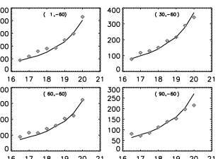
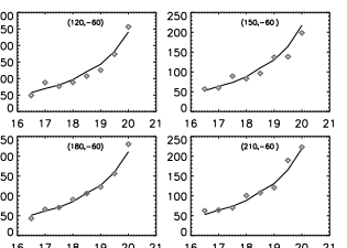
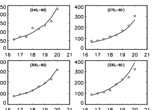
Figure 8: Model fitting to $B_{J}$ star counts in a selected sky areas whose Galactic coordinates are indicated in each panel. The grey dots are observational star counts, and the solid lines are the theoretical predictions.

Figure 9: The upper panel: Contours of $\chi^{2}$ of the theoretical models in power law index (horizontal) and axial ratio (vertical) plane. The lower panel: Contours of $\overline{\chi_{bin}^{2}}$ of the models in the same plane. The overlapped grids of the minimum contour level are labeled by diamonds, which define the best fitting model parameters.

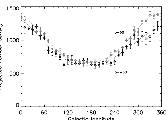
Figure 10: A direct comparison between the distributions of the surface number densities of $b=60^{\circ}$ sky areas and the $b=-60^{\circ}$ ones, with $16^{m}.5<B_{JSDSS},B_{J}<20^{m}.5$, $16^{m}.5<R_{FSDSS},R_{F}<19^{m}.5$. The black points and line represent SuperCOSMOS data of $b=-60^{\circ}$ and a polynomial fitting curve. Gray points and line are the corresponding SDSS ones.

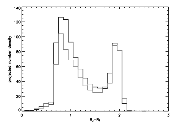
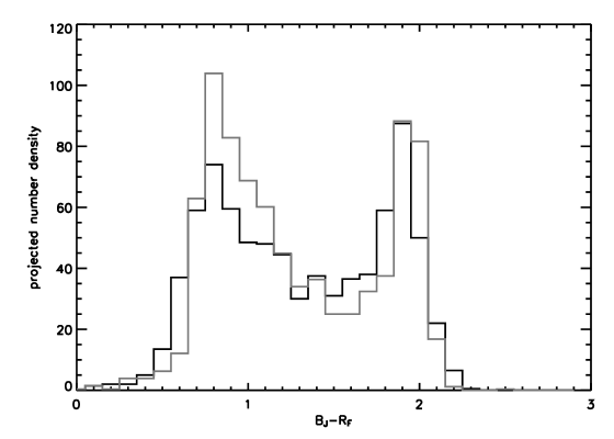
Figure 11: The upper panel: The color distribution of stars in $(l,b)=(90^{\circ},60^{\circ})$ (the gray histogram) and that in $(l,b)=(270^{\circ},60^{\circ})$ (the black histogram) for SDSS downgraded data with $16^{m}.5<B_{JSDSS}<20^{m}.5$, $16^{m}.5<R_{FSDSS}<19^{m}.5$. An overdensity due to halo stars at $(l,b)=(270^{\circ},60^{\circ})$ is shown. The lower panel: The same as the upper panel, but for $(l,b)=(90^{\circ},60^{\circ})$ (the gray histogram) of the downgraded SDSS data and $(l,b)=(90^{\circ},-60^{\circ})$ of SuperCOSMOS (the black histogram). An overdensity also due to halo stars in the north ($(l,b)=(90^{\circ},60^{\circ})$) compared to its symmetric field in the south ($(l,b)=(90^{\circ},-60^{\circ})$) is clear visible.

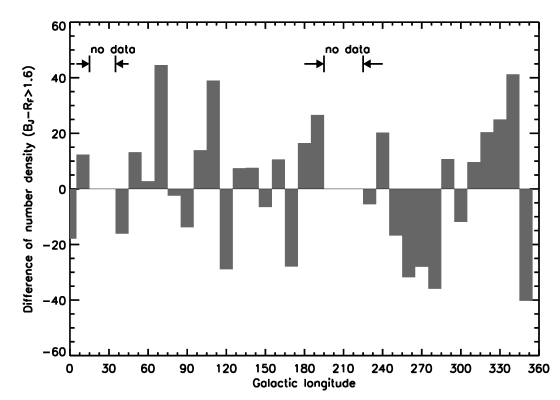
Figure 12: The difference of projected surface number densities between the sky areas along the circles in the north ($b=60^{\circ}$) and south ($b=-60^{\circ}$). Stars are selected with $16^{m}.5<B_{JSDSS},B_{J}<20^{m}.5$, $16^{m}.5<R_{FSDSS},R_{F}<19^{m}.5$. The upper panel: Data points are constrained by $0<B_{JSDSS}-R_{FSDSS},B_{J}-R_{F}<1.6$ which roughly represents the halo population. The lower panel: Data points are constrained with $1.6<B_{JSDSS}-R_{FSDSS},B_{J}-R_{F}<3.0$ which roughly represents the disk population.

References

- (1) Bahcall, J. N., Soneira, R. M., 1980, ApJS, 44,73
- Cannon (1985) Cannon R. D., 1984, in Capaccioli M. ed., Proc. IAU Colloq. 78, Astronomy with Schmidt-type Telescopes. Kluwer, Dordrecht, P. 25
- (3) Chen, B., et. al., 2001, ApJ, 553, 184
- (4) Drimmel, R., Cabrera-Lavers, A., Lpez-Corredoira, M. , 2003, A&A, 409, 205
- (5) Freeman, K., 2002, ARA&A, 40, 487
- (6) Hambly, N. C., et al., 2001a, MNRAS, 326, 1279
- (7) Hambly, N. C., Irwin, M. J., MacGillivray, H. T., 2001b, MNRAS, 326, 1295
- (8) Hambly, N. C., Davenhall, A. C., Irwin, M, J., 2001c, MNRAS, 326, 1315
- Jurić (2005) Juri, M., et al., preprint (astro-ph/0510520)
- (10) Martínez-Delgado, D., Penarrubia, J., Jurić, M., Alfaro, E. J., Ivezić, Z., preprint (astro-ph/0609104)
- (11) Newberg, H. J., Yanny, B., preprint (astro-ph/0507671)
- (12) Press, W. H., Teukolsky, S. A., Vetterling, W. T., Flannery, B. P., 1992, Numerical Recipes in Fortran: The Art of Scientific Computing. Cambridge Univ. Press, Cambridge. p. 616
- (13) Reid, N., 1993, ASPC, 49, 37
- (14) Robin, A., Crézé, M., 1986, A&A, 157,71
- (15) Xu, Y., Deng, L. C., Hu, J. Y., 2006, MNRAS, 368, 1811