Spectroscopic Survey of 1.4 GHz and 24 Micron Sources in the Spitzer First Look Survey with WIYN/Hydra

Abstract

We present an optical spectroscopic survey of 24 $\mu$m and 1.4 GHz sources, detected in the Spitzer Extragalactic First Look Survey (FLS), using the multi-fiber spectrograph, Hydra, on the WIYN telescope. We have obtained spectra for 772 sources, with flux densities above 0.15 mJy in the infrared, and 0.09 mJy in the radio. The redshifts measured in this survey are mostly in the range $0<z<0.4$, with a distribution peaking at $z\sim 0.2$. Detailed spectral analysis of our sources reveals that the majority are emission-line star-forming galaxies, with star formation rates in the range 0.2-200 M_⊙ yr^-1. The rates estimated from the H$\alpha$ line fluxes are found to be on average consistent with those derived from the 1.4 GHz luminosities. For these star-forming systems, we find that the 24 $\mu$m and 1.4 GHz flux densities follow an infrared-radio correlation, that can be characterized by a value of q₂₄ = 0.83, with a 1-sigma scatter of 0.31. Our WIYN/Hydra database of spectra complements nicely those obtained by the Sloan Digital Sky Survey, in the region at lower redshift, as well as the MMT/Hectospec survey of Papovich et al. (2006), and brings the redshift completeness to 70% for sources brighter than 2 mJy at 24 $\mu$m. Applying the classical 1/V_max method, we derive new 24 $\mu$m and 1.4 GHz luminosity functions, using all known redshifts in the FLS. We find evidence for evolution in both the 1.4 GHz and 24 $\mu$m luminosity functions in the redshift range $0<z<1$. The redshift catalog and spectra presented in this paper are available at the Spitzer FLS website.

1 Introduction

With the advent of space infrared missions in the last two decades, the understanding of galaxy formation and evolution has undergone a dramatic advance. Prior to this, the state of knowledge concerning the subject had been critically limited to the information which could be obtained mainly from the ultraviolet and optical (e.g., Lilly et al. 1995, 1996; Madau et al. 1996). While such studies allowed for some significant advances in the understanding of these processes, the sparsity of detailed information from the infrared presented a major obstacle to any significant further progress.

The relative importance of the infrared, with regard to galaxy evolution, derives primarily from the fact that the majority of light emitted by nascent stars, in the characteristically dusty star-forming regions of galaxies, is reprocessed by the surrounding dust and re-emitted at infrared wavelengths (see, e.g., Calzetti, Kinney & Storchi-Bergmann 1994). Therefore, a great deal of the information concerning star formation, its history, and hence galaxy evolution, is expected to be encoded in the infrared. In the local Universe, such infrared emission is known to constitute about one third of the total light emitted from galaxies (Soifer & Neugebauer 1991). However, as can be inferred from the cosmic background light, this contribution increases significantly with redshift, accounting for half of the total energy produced by extragalactic sources, and is due to a corresponding increase in dust-obscured star formation and/or accretion activity (Dole et al. 2006; Puget et al. 1996; see also Hauser & Dwek 2001 for a review).

With the launch of the Infrared Astronomical Satellite (IRAS) in January 1983, a number of studies of faint sources provided the first evidence for evolution in the infrared galaxy population (Hacking, Condon & Houck 1987; Lonsdale et al. 1990). However, it wasn’t until the launch of the Infrared Space Observatory (ISO) that the first detailed studies of the deep Universe were undertaken, providing new insights on galaxy evolution based on higher redshift sources. In particular, discoveries such as the excess of faint sources with respect to no-evolution models, measured in the 15 $\mu$m number counts (e.g., Elbaz et al. 1999; Flores et al. 1999; Lari et al. 2001; Metcalfe et al. 2003), led to several evolutionary models for infrared galaxies (see, e.g., Franceschini et al. 2001; Chary & Elbaz 2001; Lagache et al. 2003). In addition, an initial attempt was also made with ISO to study the 15 $\mu$m local luminosity function (Pozzi et al. 2004). However, the success of this study was somewhat hampered by the insufficient quality of the data for the task, and by limited redshift information.

More recently, the Spitzer Space Telescope opened the door to further advances and discoveries, with its significantly improved detector technology, providing both better resolution and sensitivity (Werner et al. 2004). The first survey to be performed by Spitzer, the public First Look Survey (FLS), included an extragalactic component which consisted of shallow observations of a 4.4 sq. deg. field, centered at $\alpha(2000)$ = 17^h18^m00^s, $\delta(2000)$ = 59°30′00″. The observations were obtained using the four Infrared Array Camera (IRAC) channels (Fazio et al. 2004), and the three Multiband Imaging Photometer (MIPS) bands (Rieke et al. 2004). An important aspect of the FLS was that it was also augmented by a large pool of ancillary data. Specifically, the survey was complemented at other wavelengths by Sloan Digital Sky Survey (SDSS) and Kitt Peak National Observatory (KPNO) observations, obtained in several optical bands (Hogg et al. 2007, in preparation; Fadda et al. 2004); by deeper optical and near-infrared imaging, obtained with the Canada-France-Hawaii Telescope (CFHT) and the 200 inch telescope at Palomar (Shim et al. 2006; Glassman et al. 2007, in preparation); by imaging of the same field with both the Hubble Space Telescope (HST) and the Galaxy Evolution Explorer (GALEX) (see, e.g., Bridge et al. 2007; Damjanov et al. 2006); and finally, by 1.4 GHz radio data, obtained with the Very Large Array (VLA), contributing the deepest radio survey in such a wide area to date (Condon et al. 2003).

Some of the new science made possible by this survey included the estimation of the 24 $\mu$m galaxy number counts (Marleau et al. 2004) and the MMT/Hectospec redshift survey of Papovich et al. (2006). Galaxy evolution was inferred from the 24 $\mu$m counts measured in the FLS and other deep Spitzer surveys (Marleau et al. 2004; Papovich et al. 2004), and this led to a revision of existing models (e.g., Lagache et al. 2004). Following the FLS, other Spitzer surveys were conducted to study the infrared galaxy population. For example, the 24 $\mu$m luminosity function was constructed in the Spitzer Wide-area Infrared Extragalactic (SWIRE) survey (Babbedge et al. 2006), and the Chandra Deep Field South (CDFS) and Hubble Deep Field North (HDF-N) surveys (Pérez-González et al. 2005). However, an important limitation of these studies was the fact that they were based completely on photometric redshift determination, and so lacked the reliability of spectroscopic surveys. Indeed, although multi-wavelength imaging provides a wealth of information regarding the nature of extragalactic sources, spectroscopic observations are in the end necessary to probe deeper into the nature of these sources, by providing a more accurate and detailed determination of the chemical properties, redshift distributions, luminosity functions, star-formation rates and evolutionary effects. The survey presented in this paper, which we shall now detail, aimed at doing just that.

Our program of observations and research commenced in 2002, prior to the August 2003 launch of Spitzer, with follow-up optical spectroscopy, using the Hydra spectrograph on the WIYN telescope at KPNO, and continued through until 2005. The first sources to be targeted by our survey were radio sources detected with the VLA at 1.4 GHz. Based on the infrared-radio correlation (see, e.g., Dickey & Salpeter 1984; de Jong et al. 1985; Helou et al. 1985; Condon & Broderick 1986), we expected these sources to be infrared-bright sources and, therefore, to be detected by Spitzer.

A study of the galaxy radio population offers the additional advantage that radio emission does not suffer from extinction and, therefore, is a more accurate tracer of both star formation and active galactic nuclei (AGN) activity. The 1.4 GHz luminosity function of star-forming galaxies and AGNs is well known only for the relatively local Universe (e.g., Condon, Cotton & Broderick 2002; Sadler et al. 2002). In fact, very little is known about the evolution of the radio luminosity function as, until recently, the deepest large scale radio survey reached 2.5 mJy. Moreover, attempts at measuring evolution of the radio luminosity function have remained inconclusive due to large uncertainties (Machalski & Godlowski 2000). After the FLS observations were completed in December 2003, we targeted the infrared sources detected at 24 $\mu$m with MIPS. The database of optical spectra we present in this paper provides a firm basis for the study of the bright end of the 1.4 GHz and 24 $\mu$m luminosity function, and can also be used, for example, as the training set for photometric redshifts estimation, using the neural network method (see, e.g., Collister & Lahav 2004).

The paper is organized as follows: WIYN observations and data reduction are presented in Section 2, spectral analysis and completeness of the survey are discussed in Section 3, measurement of emission lines, diagnostic diagrams and star formation rates are presented in Section 4, luminosities and the infrared-radio correlation are computed in Section 5, and in Section 6, luminosity functions at 1.4 GHz and 24 $\mu$m are derived. Section 7 describes how to access the database of the WIYN/Hydra spectra. Finally, Section 8 summarizes the main results of the paper.

Throughout this paper we assume $H_{0}=75$ km s^-1 Mpc^-1, $\Omega_{M}=0.3$, and $\Omega_{\Lambda}=0.7$.

2 Observations and Data Reduction

2.1 WIYN/Hydra Target Selection

Our WIYN/Hydra target sample was selected from two datasets of sources detected in the FLS. The first set was comprised of sources detected at 1.4 GHz and with an R-band magnitude $<23$. This set was used during our 2002 and 2003 observing runs, prior to the Spitzer launch (2003 August 25). The second set was constructed from the 24 $\mu$m sources, using the same R-band magnitude cut. These were targeted during our 2005 observing run after the Spitzer observations of the FLS were completed (2003 December 9-11). A few companions of 1.4 GHz and 24 $\mu$m sources were also part of the sample. Our list of targets was divided into 15 separate pointings (see Table 1). Each Hydra field covered a circular area 0.9 degrees in diameter, as shown in Figure 1. Note that some of the fields seen in Figure 1 are overlapping. In these fields, the source density was larger than the maximum number of allowed fibers and therefore these regions were observed more than once.

2.2 WIYN/Hydra Observational Setup

Optical spectra of the selected radio and infrared galaxies were obtained with the Hydra Multi-Object Spectrograph on the WIYN 3.5m telescope at the Kitt Peak National Observatory. Hydra has a total of 288 fiber positions (numbered $0-287$), distributed evenly around the focal plate with every third position being a red fiber. Of these $\sim$ 98 red fibers, only 93 were working properly at the time of our observations.

Each red fiber was assigned a target by taking into account a minimum fiber-to-fiber placement distance of 37 arcsec. The fibers in each field were assigned to either a target, the sky, or a guide star. On average, ten fibers were assigned to the sky in each pointing. An additional set of eleven fibers were available for guide stars. Target selection was carried out by running the assignment code whydra. The code optimized fiber placement based on a set of user-defined weights, subject to a set of fiber placement rules. Once at the telescope, the instrument program hydrawiyn made the final assignment of fibers to targets. We found that typically, $60-70$ fibers were assigned to selected survey targets in each field.

Multi-fiber spectroscopy, using 2 arcsec diameter fibers, required that the relative errors of the target coordinates be better than 0.5 arcsec. To achieve this precision, we used coordinates from the SDSS and the KPNO R-band images (Fadda et al. 2004). The relative errors in these optical catalogs were less than 0.1 arcsec. Also important was the choice of guide stars, as at least three stars were selected for each configuration. We selected guide stars with magnitudes $V=10-15$ from the Tycho2 catalog (H$\o$g et al. 2000). The coordinates had an absolute position error less than 60 milliarcseconds, allowing for accurate acquisition and guiding.

Our sample was observed on the nights of 2002 August 14-15, 2003 June 30-July 01, and 2005 July 17. We selected the $4000-9500$Å band and the red fiber set to observe emission lines from [OII] $\lambda$3727 to H$\alpha$ $\lambda$6563, for typical objects in our sample ($z\sim 0.2$). The red fiber set, combined with the Bench Spectrograph Camera, was optimized for the $4500-10000$Å wavelength range. However, because of the presence of strong sky lines, the spectra redward of $\sim$7500Å were not usable. The size of the fibers was ideally suited for our sample as each fiber covered a significant portion of a target. We used a grating with 316 lines/mm and a blaze angle of 7 degrees, yielding a dispersion of 2.64Å pixel^-1. The final resolution, measured from the FWHM of comparison lines, was $\sim$ 5Å.

Exposure sets of 3$\times$20 minutes were used for all fields. For each configuration we took dome flats and Cu-Ar comparison lamp exposures for wavelength calibration. Between each field observation, we took exposures of spectroscopic standard stars for flux calibration.

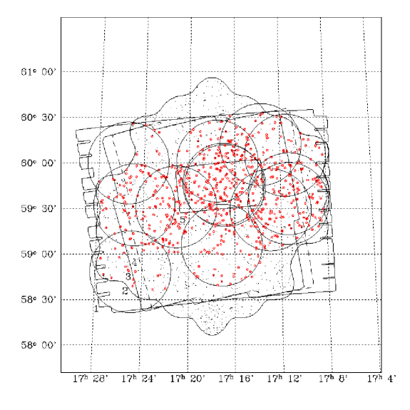
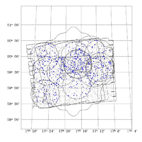
Figure 2: Left: WIYN/Hydra and Spitzer FLS fields (as described in Figure 1) and the location of the VLA radio sources (black dots) observed with WIYN/Hydra (red circles). Right: The location of the Spitzer 24 $\mu$m sources (black dots) observed with WIYN/Hydra (blue circles).

A total of 772 spectra were obtained. Figure 2 (left) shows the complete radio sample from Condon et al. (2003) and highlights the radio sources observed with WIYN/Hydra. The 24 $\mu$m sources in the FLS catalog of Fadda et al. (2006) and those targeted with WIYN/Hydra are also shown in Figure 2 (right).

2.3 WIYN/Hydra Data Reduction

The data reduction was carried out using a combination of tasks run with the Interactive Data Language (IDL) and the Image Reduction and Analysis Facility (IRAF). First, we created average dome flats and comparison arc lamps for each configuration and an average bias for each night. Images were then trimmed and the bias was subtracted. Next, we identified the hot pixels, caused by cosmic ray hits, by subtracting consecutive images and using the la_cosmic task (van Dokkum 2001). After identifying these bad pixels, we coadded all the images relative to one configuration by averaging their values and discarding the masked pixels.

Further processing of the science frames was done using the Hydra reduction package dohydra (Valdes 1995), which is specifically designed for the reduction and spectral extraction of the Hydra multi-fiber spectra. The package allows one to extract the spectra, compute and apply a flat-field and fiber throughput correction, calibrate in wavelength and subtract the sky.

To flux calibrate the spectra, the typical approach is to fit the spectrum of the standard star with a high-order polynomial. However, this removes the fine-scale features, found especially in the red part of the spectrum, making the detection of the H$\alpha$ emission lines of medium-redshift objects very difficult. Therefore, to calibrate in flux, we used a different method. We filtered the spectrum of the standard star, divided by the library spectrum, with a multiscale transform (see, e.g., Fadda, Slezak & Bijaoui 1998). This method removes the high-frequency noise and conserves the significant short-scale features. The obtained response function was then applied to the spectra. The analysis of the spectra, including redshift and line measurements, was carried out using an IDL code written by the authors. Examples of the reduced spectra are shown in Figure 3.

3 Redshift Identification

3.1 The WIYN/Hydra Survey

The redshifts of the infrared and radio sources in our WIYN survey were calculated by identifying spectral features (see Section 4 below) and taking the average. When no lines were present and the 4000Å-break was detected, the location of the break was used to determine the redshift. Of the 772 spectra, we measured redshifts for 498 extragalactic sources. Of these, eight were broad emission line objects – one of which was at $z=3.6$ (see Figure 3) – and eleven were stars. We were able to identify lines in 395 sources, whereas a redshift based on the 4000Å-break was obtained for 72 sources. The features were flagged as “break”, “emission”, or “absorption”. We visually identified the spectroscopic classification as either “galaxy”, “broad emission line”, or “star”, and assigned each target with a redshift quality assessment value of “unknown”, “tentative” or “good”. The results of the WIYN/Hydra spectroscopic survey are given in an ASCII table, available in the electronic edition of the Astrophysical Journal, with the format explained in Table 2.

Our final WIYN/Hydra redshift catalog consists of 382 radio and 412 infrared emitters, of which 322 sources are both. There are also fifteen sources with redshifts that have neither 24 $\mu$m nor 1.4 GHz flux densities (within the flux limits of the surveys). These are close companions of radio or infrared sources that make up a pair, and for which we wanted to obtain both redshifts.

3.2 Complementary Surveys

To increase the completeness of our survey at lower redshift, we queried the release 5 of the SDSS archive for the FLS region (17^h07^m $<\alpha<$ 17^h29^m, 58°21′$<\delta<$ 60°34′). A total of 812 sources with SDSS redshifts were retrieved. Of those, 70 sources were identified as WIYN/Hydra sources as well, allowing us to do a redshift comparison for a sub-sample of objects. We found excellent agreement between the WIYN/Hydra and SDSS spectroscopic redshifts, with only two cases where the redshifts are significantly ($|$z_WIYN-z${}_{MMT}|$ $>$ 0.01) discrepant. Given that these sources were classified as “tentative” under our quality index, we assigned the SDSS redshifts to these objects.

We also retrieved the MMT/Hectospec spectroscopic catalog of Papovich et al. (2006), containing 1317 measured redshifts of 24 $\mu$m sources in the FLS. In this case, we found 201 matches between the two catalogs and agreement (as defined above) for 85% of the matched sources with both redshifts measured. The discrepant 15% of the matched sources fell either under the “tentative” quality assessment or had their redshift estimated from the “4000Å-break”, which is likely less reliable than identifying features. The SDSS and MMT/Hectospec redshifts of WIYN/Hydra targets are included in Table 2.

3.3 Optical/Radio/IR Catalogs

The sources targeted by our survey were selected from both the 1.4 GHz and 24 $\mu$m FLS catalogs. The first sources to be targeted by our survey, prior to the launch of Spitzer, were radio sources detected with the VLA at 1.4 GHz. We used the catalog of Condon et al. (2003) as our 1.4 GHz FLS source list, which contained 5993 radio sources down to a flux density limit of 0.09 mJy. The 24 $\mu$m target selection was done based on the 24 $\mu$m point and extended source catalogs of Fadda et al. (2006). The point source catalog contained 16905 sources detected to a 5-sigma level (Table 5 of Fadda et al. 2006, designated as “P” in the WIYN/Hydra redshift table). An additional 124 extended sources were found in Table 2 of Fadda et al. 2006 (“E” in our table). To identify and remove stars from the point source catalog, we queried the Sloan Digital Sky Survey, Data Release 5, for stars with r’ $<$ 22. This catalog of stars was cleaned of 196 “falsely classified” stars, by matching it to all sources with a measured redshift in the FLS (derived from this work, the SDSS and the work of Papovich et al. 2006). This allowed us to clean 933 sources from our 24 $\mu$m list, leaving a total of 16096 likely extragalactic sources (extended sources included).

Compiling all the redshifts known in the FLS region, we constructed the 24 $\mu$m and 1.4 GHz all-surveys redshift catalogs. Of the 16096 sources at 24 $\mu$m  our final infrared catalog contained 412/369/1207 redshifts from WIYN/SDSS/MMT, respectively (412/305/1036 or a total of 1753 redshifts when cleaned of duplicates). Of the 5993 sources at 1.4 GHz, our final radio catalog contained 382/202/454 redshifts from WIYN/SDSS/MMT, respectively (382/151/297 or a total of 830 redshifts when cleaned of duplicates).

3.4 Redshift Distribution and Completeness of the Survey

The redshift distribution in the FLS, including our WIYN/Hydra survey, is shown in Figure 4. The majority of redshifts we measured using the WIYN/Hydra optical spectra span the range $0<z<0.4$, and the distribution peaks at $z\sim 0.2$. Also displayed in Figure 4 are the redshift distributions of the SDSS and the MMT/Hectospec survey. The WIYN/Hydra survey complements nicely the SDSS at lower redshift, as well as the MMT/Hectospec survey of Papovich et al. (2006), which covers a slightly larger redshift range.

The fraction of 1.4 GHz sources for which we successfully obtained a redshift is displayed in Figure 5 (left) as a function of flux density. A total of 641 out of the 5993 sources in this catalog were observed with WIYN/Hydra, and 382 redshifts were successfully measured, yielding a success rate of $\sim$ 60% (see Figure 5, right).

The fraction of 24 $\mu$m sources for which we successfully obtained a redshift is displayed in Figure 6, as a function of 24 $\mu$m flux density (left), and R-band magnitude (right). A redshift was successfully obtained for 412 out of the 600 sources targeted with WIYN/Hydra, i.e. with a success rate of $\sim$ 80%. The success rate is displayed in Figure 7, as a function of 24 $\mu$m flux density (left), and R-band magnitude (right). As seen in Figure 1, more 24 $\mu$m sources were targeted in the deeper FLS verification (FLSV) region. The WIYN/Hydra redshift survey is more complete there, with a success rate as shown in Figure 8.

4 Emission Line Measurements

Each emission and absorption feature was identified and fitted with a local continuum and a blend of Gaussian components, to determine line centers, fluxes, equivalent widths (EWs), and the continuum level. Errors were calculated using the raw counts. The uncorrected line strengths and equivalent widths of the principal emission features are given in an ASCII table, available in the electronic edition of the Astrophysical Journal, with the format explained in Table 3.

4.1 Extinction Correction

The comparison of the observed and predicted Balmer line ratios can be used to estimate the internal extinction of the galaxies in our survey. The H$\alpha$ $\lambda$6563 and H$\beta$ $\lambda$4861 Balmer lines, were detected in 134 WIYN/Hydra sources. Therefore, a direct measurement of the Balmer decrement was possible for this subset. For the other 317 emission-line sources, we assumed the median value of our subset of 6.26. The color excess E(B-V)_gas of each source was computed by comparing the observed Balmer line ratio (F${}_{o}^{H\alpha}$/F${}_{o}^{H\beta}$) with the intrinsic unobscured ratio using the equation

$$E(B-V)_{gas}=\frac{2.5}{[k(H\alpha)-k(H\beta)]}\log\left[\frac{F_{o}^{H\alpha}/F_{o}^{H\beta}}{F_{i}^{H\alpha}/F_{i}^{H\beta}}\right].$$ (1)

Here, the intrinsic unobscured line ratio F${}_{i}^{H\alpha}$/F${}_{i}^{H\beta}$ was set equal to 2.87, assuming case B recombination and T=10,000 K (Osterbrock 1989). The reddening curve $[k(\lambda)]$ was taken from Calzetti (2001), for starburst galaxies, and is valid between 0.12 to 2.2 $\mu$m. The color excess can also be converted into a wavelength-dependent extinction based on the relation

$$A(\lambda)=E(B-V)_{gas}\;k(\lambda),$$ (2)

where $A(\lambda)$ is the mean emission-line-derived extinction in units of magnitudes at the wavelength $\lambda$.

Using the computed color excess, all emission-lines were dereddened for each galaxy using the routine calz_unred  from the IDL astronomical library. Given the uncorrected line fluxes and color excesses, this code returns the dereddened line fluxes. The Balmer decrement, color excess and extinction, A(V), calculated for each source in our sample, can be found in an ASCII table, available in the electronic edition of the Astrophysical Journal, with the format explained in Table 4.

4.2 Diagnostic Line Ratios

Diagnostic line-intensity ratios, such as [OIII]/H$\beta$ and [NII]/H$\alpha$, corrected for reddening, are effective at separating populations with different ionization sources (Osterbrock 1989; Kewley et al. 2001). The ionizing radiation field found in active galaxies is harder than in star-forming galaxies, and this gives higher values of [NII]/H$\alpha$ and [OIII]/H$\beta$. Hence, the narrow line AGNs are found in the upper right portion of the [OIII]/H$\beta$ versus [NII]/H$\alpha$ diagnostic diagram. The lines in these ratios are also selected to be close in wavelength space in order to minimize the effect of dust extinction on the computed line ratios.

We were able to identify narrow line AGNs in our WIYN/Hydra spectroscopic sample using diagnostic diagrams of [OIII]/H$\beta$ versus [NII]/H$\alpha$ and [OIII]/H$\beta$ versus [SII]/H$\alpha$. The values of these line ratios are given in an ASCII table, available in the electronic edition of the Astrophysical Journal, with the format explained in Table 4. The results are displayed in Figure 9. At first glance, this figure reveals that the majority of emission-line sources in this subsample are star-forming systems. The theoretical starburst-AGN classification, shown in Figure 9 as the solid curve, is a result of the modeling of starburst galaxies of Kewley et al. (2001). These models are generated using the ionizing ultraviolet radiation fields produced by stellar population synthesis models (in this case PEGASE v2.0), in conjunction with a detailed self-consistent photoionization model (MAPPINGS III). Using the Kewley et al. classification, we identified twenty sources in this subsample as narrow line AGNs (shown as filled circles in Figure 9).

Sources without a [NII]/H$\beta$ flux ratio measurement were classified as AGNs when their [OIII]/H$\beta$ flux ratio was greater than 0.6 (shown as filled squares in Figure 9). This value was chosen based on the Kewley et al. curve and the median value of [NII]/H$\alpha$ for the subsample, i.e. -0.5. This is the most conservative limit of the two diagnostic diagrams. Among these sources, another eight narrow line AGNs were found, bringing the total to 28. Adding the eight broad emission line AGNs, we were able to identify, based on the properties of the optical spectra, a total of 36 AGNs in the WIYN/Hydra catalog. Identification of AGNs in the SDSS and MMT/Hectospec catalog was done using the spec_class and class index, respectively. In total, 125 and 298 AGNs were flagged in the radio and infrared catalog, respectively.

4.3 H$\alpha$ and Radio Star Formation Rates

We calculated the star formation rates (SFRs) for the 254 sources in our survey with detected H$\alpha$ line emission (corrected for extinction). We used the SDSS r’ images to estimate the aperture correction needed to transform our measured H$\alpha$ fluxes, obtained using 2 arcsec diameter fibers, to an integrated emission-line flux. The measured H$\alpha$ fluxes from HII regions can be converted into total SFRs using the H$\alpha$-SFR calibration relation derived by Kennicutt (1998)

$$SFR_{H\alpha}=7.9\times 10^{-42}L_{H\alpha},$$ (3)

where $L_{H\alpha}$ is the measured line luminosity in ergs s^-1 and the SFR_Hα is given in M_⊙ yr^-1. The conversion between ionizing flux and the star formation rate generally applies only to OB stars with masses of $>10$ M_⊙ and lifetimes $<20$ Myr. However, the conversion factor in equation (3) was extrapolated to a total SFR assuming solar abundances and a Salpeter initial mass function (IMF) over the mass range 0.1 $<$ M/M${}_{\odot}<$ 100. The main limitations of the method are its sensivity to uncertainties in extinction and the IMF (a change from Salpeter to Scalo IMF will increase the SFR by a factor of 3), and the assumption that all of the massive star formation, which contribute most to the integrated ionized flux, is traced by ionized gas. The calculated values of SFR_Hα are given in an ASCII table, available in the electronic edition of the Astrophysical Journal, with the format explained in Table 4. Note that the sources classified as AGNs were removed from this sample, as the Kennicutt relation does not apply to these systems. We estimated star formation rates in the range $0.2-200$ M_⊙ yr^-1, and found that these values were strongly correlated with extinction (see Figure 10, left).

The star formation rates can also be estimated from the radio luminosity of galaxies (see Condon 1992, equation 21 and 23). Following equation (28) of Condon, Cotton & Broderick (2002), we can write

$$SFR_{1.4~{}GHz}=1.2\times 10^{-21}L_{1.4~{}GHz},$$ (4)

where $L_{1.4~{}GHz}$ is the measured radio luminosity in W Hz^-1, and the SFR${}_{1.4~{}GHz}$ is given in M_⊙ yr^-1. The more massive stars in normal galaxies are responsible for most of the radio emission. Given that their lifetime is shorter than a Hubble time, the current radio luminosity is proportional to the recent star formation rate. The global radio non-thermal (synchrotron radiation) and thermal (free-free emission) luminosities, as well as the FIR/radio ratio, can be computed assuming an average star formation rate of stars more massive than 5 M_⊙. The star formation rate is then extrapolated to stars with M $>$ 0.1 M_⊙, by assuming a Salpeter IMF over the mass range 0.1 $<$ M/M${}_{\odot}<$ 100. The calculated values of SFR${}_{1.4~{}GHz}$ can also be found in an ASCII table, available in the electronic edition of the Astrophysical Journal, with the format explained in Table 4. As can be seen in Figure 10 (right), the SFR${}_{1.4~{}GHz}$ does not correlate with optical extinction.

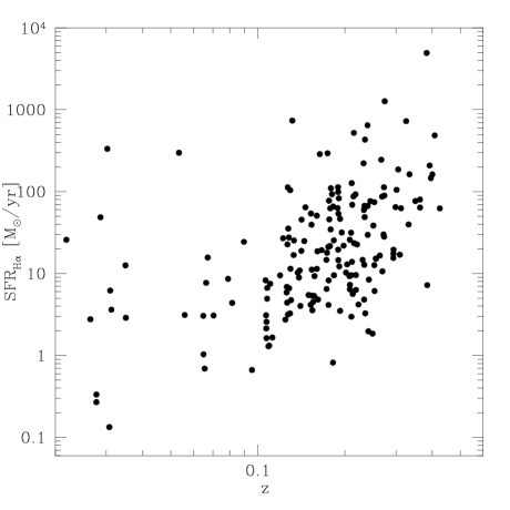
Figure 12: Star formation rates computed from H$\alpha$ (left) and 1.4 GHz luminosities (right) as a function of redshift.

The star formation rates derived from the H$\alpha$ and 1.4 GHz luminosities are compared in Figure 11. The star formation rate computed from the radio luminosity is on average consistent with the one derived from the H$\alpha$ optical line emission. The star formation rates start to deviate slightly from this simple correlation at the upper end of the SFR range, as the optical extinction increases (see Figure 10, left), and therefore the H$\beta$ flux measurement becomes more uncertain. Moreover, we don’t necessarily expect a perfect agreement between the two methods as the current radio emission is proportional to the rate of massive star formation occuring during the past 100 Myr, whereas the H$\alpha$ line emission is associated with more recent, i.e. $<20$ Myr, star-forming activity. The star formation rates are plotted as a function of redshift in Figure 12. At low redshift ($z<0.4$), our survey is detecting sources with a wide range of star-forming activity. However, at higher redshifts, we are only detecting sources with a SFR $>40$ M_⊙ yr^-1.

5 Luminosities and Infrared-Radio Correlation

Radio and infrared luminosities were calculated for a total of 830 radio sources and 1753 24 $\mu$m sources. The observed radio flux densities were corrected to the rest-frame flux densities by applying a multiplicative factor of $(1+z)^{0.7}$, assuming a power law emission of $S\propto\nu^{-0.7}$ at these frequencies. The flux densities were also corrected for the effect of bandwidth compression by applying the multiplicative term of $(1+z)^{-1}$.

The k-correction for the 24 $\mu$m passband was computed using redshifted spectral energy distribution (SED) templates. The majority of 24 $\mu$m sources are star forming galaxies, but their SEDs are not known a priori. However, if fluxes are also measured at other wavelengths, such as 4.5, 24 and 70 $\mu$m, it becomes possible to select a best fit SED from a database of SEDs, such as the one of Siebenmorgen & Krügel (2007), and compute a correction specific to each source. To see if we could apply this technique, we used the 70 $\mu$m source catalogs of Frayer et al. (2004). Unfortunately, only 22% of all sources with measured redshifts were detected at 70 $\mu$m. With most of the 24 $\mu$m population unknown, and with luminosities in the range of normal star-forming galaxies, we therefore elected to use the SED of the typical starburst galaxy M82 as our template for calculating the k-correction (data from Sturm et al. 2000). We obtained identical results when using the average IRS spectrum of 13 starburst galaxies (Brandl et al. 2006). As can be seen in Figure 6 of Brandl et al. (2006), this is not surprising, as this average IRS spectrum and the M82 SED are virtually the same at these wavelengths.

However, extreme sources, such as high redshift luminous infrared galaxies (LIRGs), ultra-luminous infrared galaxies (ULIRGs) and AGNs, are not expected to be well represented by this template. To estimate the error on the luminosity calculations at the bright end of the luminosity function of star forming galaxies, we re-computed the k-correction using two additional templates: UGC 5101 (data from Armus et al. 2007), a typical ULIRG, and Arp 220 (data from Sturm et al. 1996), one of the most extreme objects of this type (see Figure 2 of Armus et al. 2007). The 24 $\mu$m luminosities computed using the M82 and Arp 220 templates differed by $<2$ %, over the redshift range of our survey. The difference was even less when comparing to our typical ULIRG, UGC 5101. Similarly, the impact on the measurement of q₂₄ (see below) was found to be insignificant; using Arp 220, we found a difference of 0.8 % in the median and 0.2 % in the dispersion. The use of M82 for the k-correction was therefore found to be completely adequate for our sample. Moreover, this result is consistent with the work of Appleton et al. (2004), who performed a comparison between the k-correction computed from best fit model SEDs and the SED of M82. We stress, however, that this assumption is likely to break down at higher redshifts, i.e. $z>1.2$, when differences in the SEDs start to have a large impact on the 24 $\mu$m flux densities. As for the AGNs identified in our sample, the Circinus galaxy, a Seyfert 2 object, was assumed as a typical template and used to compute the k-correction (data from Sturm et al. 2000).

The luminosity distribution of the radio sources from our WIYN survey is shown as a function of redshift in Figure 13 (left). The majority of galaxies detected in the redshift range $z=0-0.4$ have low to medium radio luminosities, typical of star-forming galaxies, whereas almost all the higher redshift galaxies are of higher radio luminosity, comparable with powerful luminous infrared galaxies and radio-quiet quasars. The 0.09 mJy flux density limit of the radio survey (solid line in Figure 13, left) tends to truncate the shape of the luminosity function at $z>0.3$. The 24 $\mu$m luminosity distribution is also shown in Figure 13 (right), along with its flux density limits (50% completeness limits) of 0.3 mJy, for the FLS main (FLS) data, and 0.15 mJy, for the deeper FLS verification (FLSV) observations. We plotted the optical extinction as a function of 1.4 GHz and 24 $\mu$m luminosity for the 134 WIYN/Hydra sources with measured H$\alpha$ and H$\beta$ fluxes. No obvious trend was seen. The optical extinction does not appear to correlate with redshift either.

For star-forming galaxies, there exists a tight correlation between far-infrared and radio luminosity. However, as shown by Appleton et al. (2004), this correlation shows much larger scatter when 24 $\mu$m flux densities are used. The monochromatic 24 $\mu$m infrared-radio correlation can best be plotted as a function of redshift by computing the parameter

$$q_{24}=\log(S_{24{\mu}m}/S_{1.4~{}GHz}),$$ (5)

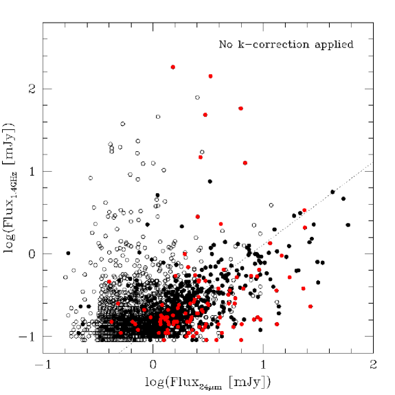
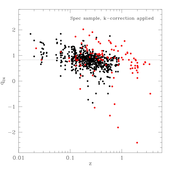
Figure 14: Left: Relation between 24 $\mu$m and 1.4 GHz raw flux densities, i.e. no k-correction applied (open circles). The sources with redshifts are shown with filled black circles and the optically classified AGNs are identified as filled red circles. The dotted line represents the median value of q₂₄ = 0.89, measured using the uncorrected flux densities. Right: The parameter q₂₄, computed using k-corrected flux densities, as a function of redshift for star-forming galaxies (filled black circles). The AGNs that we have identified in the WIYN/Hydra, SDSS and MMT catalogs are shown as filled red circles. The dotted line represents the median value of q₂₄ = 0.83.

where $S_{24{\mu}m}$ and $S_{1.4~{}GHz}$ is the flux density in the 24 $\mu$m band and at 1.4 GHz, respectively. The median value of q₂₄ is a measure of the slope of the infrared-radio correlation, whereas the dispersion is related to the strength of the correlation for the given sample of galaxies. For our WIYN/Hydra sources, the 1.4 GHz and 24 $\mu$m raw flux densities, i.e. no k-correction applied, are plotted against each other in Figure 14 (left). Using these uncorrected flux densities, we calculated the median value of q₂₄ to be 0.89, with a dispersion of 0.30. The values of q₂₄ were also computed using k-corrected flux densities and are plotted against redshift in Figure 14 (right). Removing the optically classified AGNs, we measured the median value to be q₂₄ = 0.83, with a 1-sigma dispersion of 0.31, in agreement with Appleton et al. (2004). This is not too surprising as there is some overlap between our sample and the one of Appleton et al. (2004), although the latter is derived mostly from Keck/DEIMOS redshifts (see Choi et al. 2006). From Figure 14 (right), we can see that there is clearly a population of radio-loud AGN objects which falls off the correlation. These sources were not classified as optical AGNs. They are possibly buried AGNs, or sources that have not been corrected properly using the M82 template for the 24 $\mu$m luminosity calculation. The former explanation is most probably correct, as this population is also seen when the raw flux densities are plotted (Figure 14, left). We also note a slight tendancy for the radio-quiet AGNs to lie below the average correlation, i.e. higher q₂₄ (see Figure 14, left). This effect, however, is less noticeable when the k-correction is applied (see Figure 14, right). It is not clear how significant this is, since the k-corrected 24 $\mu$m flux densities depend on the assumed infrared SED, mostly for the high redshift sources.

6 Radio and Infrared Luminosity Functions

The 1.4 GHz and 24 $\mu$m luminosity functions (LFs) are computed using the $1/V_{max}$ method (Schmidt 1968). $V_{max}$ is the maximum volume within which a galaxy at redshift $z$ could be detected by our survey, given the flux density limits of $f^{lim}_{1.4~{}GHz}=$ 0.09 mJy and $f^{lim}_{24{\mu}m}=$ 0.3 mJy, and the optical limits of R $<$ 23 (WIYN/Hydra) and $i^{\prime}<21.3$ (SDSS and MMT/Hectospec). The maximum comoving volume is given by

$$V_{max}=(\omega/3)d_{M}^{3},$$ (6)

where $\omega$ is the solid angle subtended by the FLS 4.4 sq. deg. area, and $d_{M}$ is the proper motion distance defined as

$$d_{M}=\frac{c}{H_{0}}\int_{z_{min}}^{z_{max}}\frac{dz}{\sqrt{(1+z)^{2}(1+\Omega_{M}z)-z(2+z)\Omega_{\Lambda}}}.$$ (7)

Here, $z_{min}$ and $z_{max}$ refer to the minimum and maximum redshifts (see, e.g., Carroll, Press & Turner 1992). In our survey, $z_{min}=0$ and $z_{max}$ can be computed from $d_{L}(z_{max})=d_{L}(z)$ [$f_{24{\mu}m}/f^{lim}_{24{\mu}m}$] (IR sample), or $d_{L}(z_{max})=d_{L}(z)$ [$f_{1.4~{}GHz}/f^{lim}_{1.4~{}GHz}$] (radio sample), where $d_{L}(z)$, the luminosity distance at redshift $z$, is equal to $(1+z)d_{M}(z)$.

The density of sources in a given luminosity bin of width $\Delta\log L$, centered on luminosity $\log L_{i}$, is simply the sum of the inverse volumes $1/V_{max}$ of all the sources with luminosities in the bin. The luminosity function is expressed as

$$\phi(\log L_{i})=\frac{1}{\Delta\log L}\sum_{|\log L_{j}-\log L_{i}|<\Delta\log L}\frac{1}{V_{max,j}},$$ (8)

where the index $i$ labels luminosity bins, the index $j$ labels galaxies, and
$1/V_{max,j}$=min($V_{optical,j},V_{24{\mu}m,j}$) (IR sample), or $1/V_{max,j}$=min($V_{optical,j},V_{1.4~{}GHz,j}$) (radio sample). Since Poisson statistics apply, the root-mean-square error is

$$\Delta\phi(\log L_{i})=\frac{1}{\Delta\log L}\sqrt{\sum_{|\log L_{j}-\log L_{i}|<\Delta\log L}\frac{1}{V^{2}_{max,j}}}.$$ (9)

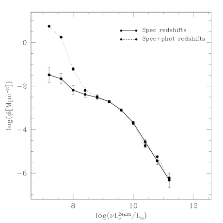
Figure 15: The 1.4 GHz (left) and 24 $\mu$m (right) luminosity function for star-forming galaxies in the FLS. Note that incompleteness corrections have not been made (solid lines). The luminosity functions with added SDSS photometric redshifts, where the AGN component was removed statistically, are shown as the dotted lines.

In Figure 15 we show our derived 1.4 GHz and 24 $\mu$m luminosity functions for star-forming galaxies in the FLS. A total of 125 and 298 AGNs were removed from the radio and 24 $\mu$m all redshift catalogs, respectively. The luminosity function is plotted as a function of $\log(\nu L_{\nu}/L_{\odot})$, with bin width defined as $\Delta\log(\nu L_{\nu}/L_{\odot})=0.4$. The values are listed in Table 5 and 6. The luminosity functions presented in this paper have not been corrected for incompleteness. A future paper will be dedicated to a more indepth study of the luminosity functions, and will exploit a new set of spectra of fainter galaxies (obtained with the Keck telescope) and photometric redshift estimates for the remaining sources.

Nevertheless, a preliminary estimate of the incompleteness correction at low redshift is presented here. We queried the SDSS archive for photometric redshifts in the FLS region. A total of 58321 sources with SDSS photometric redshifts were retrieved. We matched our 24 $\mu$m and 1.4 GHz source lists with the SDSS photometric redshift catalog and found 8441 and 2348 matches, respectively. As the SDSS photometric redshift catalog is contaminated by AGNs, we corrected the luminosity function with added photometric redshifts by applying a correction factor, derived from the measured fraction of AGNs per luminosity bin in our spectroscopic sample. The results are shown in Figure 15 as the dotted lines. As we are less complete at 1.4 GHz than at 24 $\mu$m (see Figure 5 and 6), the completeness correction is more important in the radio.

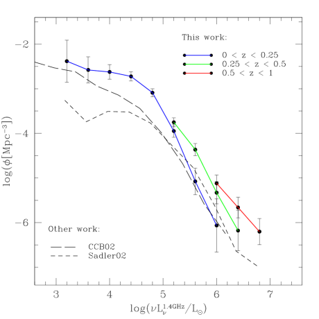
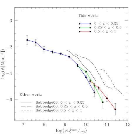
Figure 16: The 1.4 GHz (left) and 24 $\mu$m (right) luminosity function for star-forming galaxies in the FLS, split into the redshift bins $z=0-0.25$ (blue line), $0.25-0.5$ (green line), and $0.5-1.0$ (red line). On the left, our 1.4 GHz luminosity function is compared to the 1.4 GHz local luminosity function of Condon, Cotton & Broderick (2002) (long-dash line) and the luminosity function of Sadler et al. (2002) (short-dash line). On the right, our 24 $\mu$m luminosity function is compared to the 24 $\mu$m luminosity function of Babbedge et al. (2006) for the redshift bins $z=0-0.25$ (solid line), $0.25-0.5$ (long-dash line), and $0.5-1.0$ (short-dash line).

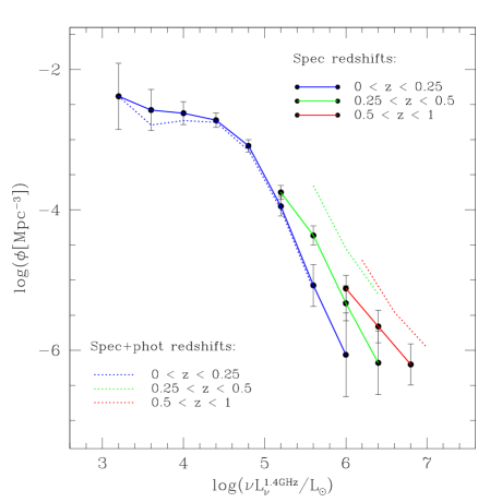
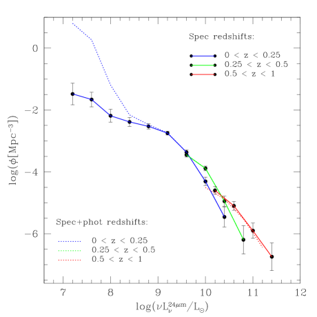
Figure 17: The 1.4 GHz (left) and 24 $\mu$m (right) luminosity function for star-forming galaxies in the FLS, split into the redshift bins $z=0-0.25$ (blue line), $0.25-0.5$ (green line), and $0.5-1.0$ (red line). The dotted colored lines refer to the luminosity function with added SDSS photometric redshifts, where the AGN component was removed statistically, for the same redshift bins.

Both luminosity functions are split into the redshift bins $z=0-0.25$, $0.25-0.5$, and $0.5-1.0$, to investigate evolution in the 24 $\mu$m and 1.4 GHz sample (see Figure 16). We compare our 24 $\mu$m luminosity function with the luminosity function of Babbedge et al. (2006), based on photometric redshifts. Our luminosity functions are lower than those of Babbedge et al. (2006), even when the photometric redshifts are included (Figure 17, dotted lines). This is not surprising, as our luminosity functions are not corrected for incompleteness. The 1.4 GHz luminosity function derived for the redshift bin $z=0-0.25$ agrees well with the 1.4 GHz local luminosity function of Condon, Cotton & Broderick (2002) and Sadler et al. (2002) at the bright end, and is larger at fainter luminosities. This difference can be explained by the lower flux density limit of our survey (0.09 mJy compared to 2.5 mJy). Moreover, the greater depth of our radio survey, compared to previous surveys, allows us to present the first 1.4 GHz luminosity functions at high redshift (see Figure 16). Luminosity evolution over the redshift range $z=0-1$ is clearly detected in both 1.4 GHz and 24 $\mu$m luminosity functions, as shown in Figure 16. This is very interesting as it shows that the infrared and radio galaxy populations were forming stars more actively in the past, like the ultraviolet and optical populations (e.g., Lilly et al. 1995, 1996; Madau et al. 1996), and that therefore this increase in activity at earlier times appears to be a generic property of galaxies.

We also make use of the $V/V_{max}$ method (Schmidt 1968) to test the evolution of the uniformity of the space distribution of sources. The volume, $V$, is the volume corresponding to the actual redshift at which the source is observed and, therefore, the ratio $V/V_{max}$ is a measure of the position of the source within the observable volume, $V_{max}$. The distribution of sources is uniform if $V/V_{max}$ has a uniform distribution from 0 to 1, or the mean value of $V/V_{max}=0.5$. We compute a mean value of $V/V_{max}=0.34\pm 0.26$ and $0.41\pm 0.24$ at 24 $\mu$m and 1.4 GHz, respectively. Although the upper limits are consistent with a luminosity evolution, their low values are indicative of completeness issues and, therefore, cannot be used reliably until incompleteness corrections have been applied.

7 Database of Spectra

The electronic edition of this publication contains the WIYN/Hydra redshift catalog and line measurements, i.e. Table 2, 3 and 4. The reduced spectra can be obtained from the Spitzer FLS website.

8 Summary

We presented an extensive redshift survey of 1.4 GHz and 24 $\mu$m sources in the FLS main and verification fields. We observed 772 sources, and measured redshifts for 382 radio and 412 infrared sources, adding up to 498 redshifts. In the deeper FLS verification region, our survey is 100% complete for 24 $\mu$m flux densities $>$ 0.2 mJy. The success rate of redshift identification of 24 $\mu$m sources is $\sim$ 80%. For the radio sources, our redshift success rate is slightly lower ($\sim$ 60%). The WIYN/Hydra redshift catalog and line measurements are available with the online version of this publication. The reduced spectra can be obtained from the Spitzer FLS website.

Our spectroscopic and emission-line survey covered mainly redshifts in the range $0<z<0.4$, with a distribution peaking at $z\sim 0.2$. Most of our WIYN/Hydra sources are galaxies, with eight broad emission line objects, one of which is a quasar at $z=3.6$. Using the diagnostic line ratios, to separate starburst from AGNs, we found an additional 28 sources with AGN-like emission properties.

The Balmer decrement was used to correct emission line fluxes for extinction. We calculated the SFRs for the subset of our sample with measured H$\alpha$ fluxes. We found that star formation rates computed from the H$\alpha$ line flux measurements ranged from 0.2-200 M_⊙ yr^-1, and correlated directly with extinction. The star formation rates derived from the radio luminosities were found to be on average consistent with those estimated using the H$\alpha$ line fluxes. Moreover, they did not correlate with optical extinction. At low redshift ($z<0.4$), our survey detected sources with a wide range of star-forming activity. However, at higher redshifts, we only detected sources with a SFR $>40$ M_⊙ yr^-1.

We complemented our redshift database with the redshifts produced by the SDSS and MMT surveys, yielding a total of 830 redshifts for the 1.4 GHz sources and 1753 for the 24 $\mu$m sources. The 1.4 GHz and 24 $\mu$m luminosity of sources in the FLS was computed for all galaxies with a redshift. The majority of galaxies in the redshift range $z=0-0.4$ were found to have low to medium radio luminosity, typical of star-forming galaxies, whereas almost all the higher redshift galaxies had higher radio luminosities, comparable to powerful luminous infrared galaxies and radio-quiet quasars. The infrared-radio correlation was derived and a median value of $q_{24}$ = 0.83 was measured, with a 1-sigma dispersion of 0.31.

The 24 $\mu$m and 1.4 GHz luminosity functions – uncorrected for incompleteness – were derived from this spectroscopic sample. By splitting our sample into the redshift bins $z=0-0.25$, $0.25-0.5$, and $0.5-1.0$, we found evidence for luminosity evolution in both the 1.4 GHz and 24 $\mu$m luminosity functions.

Table 1: The 15 Fields Observed with WIYN/Hydra.

Field	$\alpha$ (J2000.0)	$\delta$ (J2000.0)	Observation Date (UTC)
FLS1a02	17:17:00.000	+59:46:00.00	2002 Aug 14
FLS1b02	17:16:52.056	+59:45:00.00	2002 Aug 14
FLS1c02	17:21:07.881	+59:31:00.00	2002 Aug 14
FLS2a02	17:21:07.881	+59:31:00.00	2002 Aug 15
FLS2b02	17:12:52.119	+59:29:00.00	2002 Aug 15
FLS2c02	17:16:52.060	+59:45:00.00	2002 Aug 15
FLS1a03	17:11:35.376	+60:04:59.91	2003 Jun 30
FLS1b03	17:13:45.307	+60:12:01.32	2003 Jun 30
FLS1c03	17:11:16.641	+59:39:38.39	2003 Jun 30
FLS2a03	17:11:18.700	+59:33:15.20	2003 Jul 01
FLS2b03	17:17:08.560	+59:05:48.00	2003 Jul 01
FLS2c03	17:17:31.600	+60:01:04.00	2003 Jul 01
FLS2d03	17:24:48.630	+59:32:16.00	2003 Jul 01
FLS1a05	17:25:10.218	+58:48:15.00	2005 Jul 17
FLS1b05	17:25:19.624	+59:59:53.30	2005 Jul 17

Table 2: Format of the WIYN/Hydra Spectroscopic Catalog of 1.4 GHz and 24 Micron Sources in the Spitzer FLS

Column	Format	Description
1:3	i3	ID
5:11	a7	Field (as defined in Table 1)
13:18	a6	APID
20:39	a20	WIYN/Hydra Target RA,Dec (J2000)
41:49	f7.4	WIYN/Hydra Redshift
49:54	f6.4	WIYN/Hydra Redshift Error
56:56	i1	WIYN/Hydra Redshift Quality
		[0:unknown, 1:tentative, 2:good]
58:60	a3	WIYN/Hydra Type of Spectrum
		[sta:star, gal:galaxy, bel:broad emission line]
62:67	a6	WIYN/Hydra Features
		[b:break, e:emission, a:absorption]
69:74	f6.2	Optical Counterpart R-Band Magnitude
76:95	a20	Radio 1.4 GHz/20 cm Counterpart RA,Dec (J2000)
97:103	f7.3	Radio Counterpart 1.4 GHz/20 cm Flux Density [mJy]
105:110	f6.3	Radio Counterpart 1.4 GHz/20 cm Flux Density Error [mJy]
112:116	f5.2	WIYN/Radio Match Separation [arcsec]
118:137	a20	FIR 24 $\mu$m Counterpart RA,Dec (J2000)
139:143	f5.2	FIR Counterpart 24 $\mu$m Flux Density [mJy]
145:149	f5.2	FIR Counterpart 24 $\mu$m Flux Density Error [mJy]
151:155	f5.2	WIYN/FIR Match Separation [arcsec]
157:157	a1	FIR Source Type
		[E:extended, P:point source, -:no match]
159:165	f7.4	SDSS Redshift
167:173	f7.4	MMT Redshift

Table 3: Format of the Uncorrected Line Strengths and Equivalent Widths Table

Column	Format	Description
1:3	i3	ID
5:11	a7	Field (as defined in Table 1)
13:18	a6	APID
20:39	a20	WIYN/Hydra Target RA,Dec (J2000)
41:46	f6.1	CIII $\lambda$1909 Flux [1e-17 erg/cm2/s]
48:53	f6.1	CIII $\lambda$1909 EW [Å]
55:60	f6.1	MgII $\lambda$2798 Flux [1e-17 erg/cm2/s]
62:67	f6.1	MgII $\lambda$2798 EW [Å]
69:74	f6.1	H$\beta$ $\lambda$4861 Flux [1e-17 erg/cm2/s]
76:81	f6.1	H$\beta$ $\lambda$4861 EW [Å]
83:88	f6.1	[OIII] $\lambda$5007 Flux [1e-17 erg/cm2/s]
90:95	f6.1	[OIII] $\lambda$5007 EW [Å]
97:102	f6.1	H$\alpha$ $\lambda$6563 Flux [1e-17 erg/cm2/s]
104:109	f6.1	H$\alpha$ $\lambda$6563 EW [Å]
111:116	f6.1	[NII] $\lambda$6583 Flux [1e-17 erg/cm2/s]
118:123	f6.1	[NII] $\lambda$6583 EW [Å]
125:130	f6.1	[SII] $\lambda$6716 Flux [1e-17 erg/cm2/s]
132:137	f6.1	[SII] $\lambda$6716 EW [Å]
139:144	f6.1	[SII] $\lambda$6731 Flux [1e-17 erg/cm2/s]
146:151	f6.1	[SII] $\lambda$6731 EW [Å]

Table 4: Format of the Dereddened Line Ratios and Extinction Table

Column	Format	Description
1:3	i3	ID
5:11	a7	Field (as defined in Table 1)
13:18	a6	APID
20:39	a20	WIYN/Hydra Target RA,Dec (J2000)
42:47	f7.2	Balmer Decrement ($F_{o}^{H\alpha}/F_{o}^{H\beta}$)
49:55	f7.2	Color Excess E(B-V) [mag]
57:63	f7.2	Extinction A(V) [mag]
65:71	f7.2	Dereddened H$\alpha$ Luminosity log([erg/s])
73:79	f7.2	1.4 GHz Luminosity log([W/Hz])
81:87	f7.2	24 $\mu$m Luminosity log([W/Hz])
89:95	f7.2	SFRHα [M⊙ yr-1]
97:103	f7.2	SFR${}_{1.4~{}GHz}$ [M⊙ yr-1]
105:111	f7.2	log([OIII] $\lambda$5007/H$\beta$ $\lambda$4861)
113:119	f7.2	log([NII] $\lambda$6583/H$\alpha$ $\lambda$6563)
121:127	f7.2	log([SII] $\lambda$6716+6731/H$\alpha$ $\lambda$6563)

Table 5: The 1.4 GHz LF in the FLS from the 1/$V_{max}$ Analysis

$\log(\nu L_{\nu}^{1.4~{}GHz}/L_{\odot})$	$\log(\phi[$Mpc${}^{-3}])$	1$\sigma$ error
3.2	-2.38	0.47
3.6	-2.58	0.29
4.0	-2.62	0.16
4.4	-2.72	0.10
4.8	-3.02	0.08
5.2	-3.54	0.08
5.6	-4.14	0.10
6.0	-4.88	0.15
6.4	-5.52	0.20
6.8	-6.16	0.28
7.2	-7.12	0.58

Table 6: The 24 $\mu$m LF in the FLS from the 1/$V_{max}$ Analysis

$\log(\nu L_{\nu}^{24\mu m}/L_{\odot})$	$\log(\phi[$Mpc${}^{-3}])$	1$\sigma$ error
7.2	-1.48	0.35
7.6	-1.66	0.24
8.0	-2.18	0.21
8.4	-2.39	0.14
8.8	-2.53	0.09
9.2	-2.71	0.06
9.6	-3.10	0.05
10.0	-3.68	0.06
10.4	-4.56	0.10
10.8	-5.44	0.17
11.2	-6.32	0.33

Figure 1: Coverage of 1) infrared Spitzer MIPS-24 $\mu$m main FLS field (Fadda et al. 2006), 2) VLA 1.4 GHz (Condon et al. 2003), 3) infrared Spitzer IRAC channels 1 and 3 (Lacy et al. 2005), 4) infrared Spitzer IRAC channels 2 and 4 (Lacy et al. 2005), and 5) infrared Spitzer MIPS-24 $\mu$m deeper FLS verification region (Fadda et al. 2006). The solid circles outline the 15 fields (see Table 1) where our WIYN/Hydra spectroscopic targets were selected.

Figure 3: Example spectra from our WIYN/Hydra optical spectroscopic survey. From top to bottom: an emission line galaxy at $z=0.12$, an early-type galaxy at $z=0.22$, a broad emission line object at $z=0.06$, and a quasar at $z=3.6$.

Figure 4: Top: Redshift distribution of radio and 24 $\mu$m sources observed by the SDSS (dotted line), with WIYN/Hydra (solid line) and with the MMT/Hectospec (short-dash line). Bottom: R-band magnitude and redshift correlation for the SDSS (crosses), WIYN/Hydra (filled triangles) and MMT (diagonal crosses) redshifts. The WIYN/Hydra survey had a magnitude limit of R $<$ 23, corresponding roughly to a redshift limit of z $<$ 0.8.

Figure 5: Left: Fraction of 1.4 GHz sources with spectroscopic redshifts in the FLS as a function of flux density. Right: Fraction of WIYN/Hydra targets for which we have successfully measured a redshift as a function of their 1.4 GHz flux density.

Figure 6: Left: Fraction of 24 $\mu$m sources with spectroscopic redshifts in the FLS as a function of 24 $\mu$m flux density. The stars were removed from the 24 $\mu$m catalog. Right: Fraction of 24 $\mu$m sources with redshift in the FLS as a function of R-band magnitude. Our magnitude cutoff for our survey was an R-band magnitude of 23.

Figure 7: Fraction of WIYN/Hydra targets for which we have successfully measured a redshift as a function of 24 $\mu$m flux density (left) and R-band magnitude (right).

Figure 8: Fraction of 24 $\mu$m sources with spectroscopic redshifts in the FLS verification region only, where our redshift survey is more complete, as a function of 24 $\mu$m flux density (left) and R-band magnitude (right).

Figure 9: [OIII]/H$\beta$ vs. [NII]/H$\alpha$ diagnostic diagram (left) and [OIII]/H$\beta$ vs. [SII]/H$\alpha$ (right), for the WIYN/Hydra spectroscopic sources where these emission lines were detected. HII region-like objects are plotted with open circles, whereas objects classified as narrow line AGNs are shown as filled circles. The solid line is the theoretical starburst-AGN classification line from Kewley et al. (2001). The dotted line shows the error range of the Kewley et al. model predictions ($\pm 0.1$ dex range of solid line).

Figure 10: Left: Optical extinction versus SFR measured from H$\alpha$, for the WIYN/Hydra sources with measured H$\alpha$ and H$\beta$ fluxes. The AGNs, as selected from the diagnostic line ratios, were removed. Right: Optical extinction versus SFR estimated from the radio luminosity.

Figure 11: Comparison between the star formation rates computed from the H$\alpha$ and 1.4 GHz luminosities. All sources with dereddened H$\alpha$ fluxes and detected at 1.4 GHz are shown as open circles. The filled circles designate the sources for which a Balmer decrement was measured directly (otherwise, the median value of 6.26 was assumed). The dotted line is the linear relationship with zero intercept and slope equals to one.

Figure 13: Left: The distribution of radio luminosities with redshift in the Spitzer FLS region for SDSS (crosses), WIYN (filled triangles) and MMT (diagonal crosses), from our 1.4 GHz and 24 $\mu$m-selected sample. For comparison, we show the relative scaling between the radio and FIR flux densities (left- and right-hand scale, respectively), assuming a value of q=2.32 for the slope of the radio-FIR correlation (Helou et al. 1985). This value is only appropriate for star-formation dominated systems. The solid line shows the 5$\sigma$ flux density limit of the radio survey. Right: The distribution of 24 $\mu$m luminosities with redshift. The 50% completeness limit of the FLS (solid line) and FLSV (long-dash line) are also shown.

References

- (1) Abazajian, K., et al. 2004, AJ, 128, 502
- (2) Appleton, P.N., et al. 2004, ApJS, 154, 147
- (3) Armus, L., et al. 2007, ApJ, 656, 148
- (4) Babbedge, T.S.R., et al. 2006, MNRAS, 370, 1159 (Babbedge06)
- (5) Brandl, B.R., et al. 2006, ApJ, 653, 1129
- (6) Bridge, C.R., Appleton, P.N., Conselice, C.J., Choi, P.I, Armus, L., Fadda, D., Laine, S., Marleau, F.R., Carlberg, R.G., Helou, G., Yan, L. 2007, ApJ, in press, astro-ph/0701040
- (7) Calzetti, D., Kinney, A.L. & Storchi-Bergmann, T. 1994, ApJ, 429, 582
- (8) Calzetti, D. 2001, PASP, 113, 1449
- (9) Carroll, S.M., Press, W.H., & Turner, E.L. 1992, ARA&A, 30, 499
- (10) Collister, A.A. & Lahav, O. 2004, PASP, 116, 345
- (11) Chary, R. & Elbaz, D. 2001, ApJ, 556, 562
- (12) Choi, P.I., et al. 2006, ApJ, 637, 227
- (13) Condon, J.J., & Broderick, J.J. 1986, AJ, 92, 94
- (14) Condon, J.J. 1992, ARA&A, 30, 575
- (15) Condon, J.J., Cotton, W.D., & Broderick, J.J. 2002, AJ, 124, 675 (CCB02)
- (16) Condon, J.J., et al. 2003, AJ, 125, 2411
- (17) Damjanov, I., Fadda, D., Marleau, F.R., Appleton, P.N., Choi, P.I., Lacy, M., Storrie-Lombardi, L.J., Yan, L. 2006, astro-ph/0604276
- (18) de Jong, T., Klein, U., Wielebinshi, R., & Wunderlich, E. 1985, A&A, 147, L6
- (19) Dickey, J.M., & Salpeter, E.E. 1984, ApJ, 284, 461
- (20) Dole, H., et al. 2006, A&A, 451, 417
- (21) Elbaz, D., et al. 1999, A&A, 351, L37
- (22) Fadda, D., et al. 2006, AJ, 131, 2859
- (23) Fadda, D., et al. 2004, AJ, 128, 1
- (24) Fadda, D., et al. 2002, A&A, 383, 838
- (25) Fadda, D., Slezak, E., & Bijaoui, A. 1998, A&AS, 127, 335
- (26) Fazio, G.G., et al. 2004, ApJS, 154, 10
- (27) Flores, H., et al. 1999, ApJ, 517, 148
- (28) Franceschini, A., et al. 2001, A&A, 378, 1
- (29) Frayer, D., et al. 2004, ApJS, 154, 137
- (30) Glassman, T., et al. 2007, in preparation
- (31) Hacking, P.B., Condon, J.J., & Houck, J.R. 1987, ApJL, 316, 15
- (32) Hauser, M.G., & Dwek, E. 2001, ARA&A, 39, 249
- (33) Helou, G., et al. 1985, ApJ, 298, L7
- (34) Hogg, D.W., et al. 2007, in preparation
- (35) Hg, E. et al. 2000, A&A, 355, 27
- (36) Kennicutt, R.C. 1998, ARA&A, 36, 189
- (37) Kewley, L.J., Dopita, M.A., Sutherland, R.S., Heisler, C.A., Trevena, J. 2001, ApJ, 556, 121
- (38) Lacy, M., et al. 2005, ApJS, 161, 41
- (39) Lagache, G., et al. 2003, MNRAS, 338, 555
- (40) Lagache, G., et al. 2004, ApJS, 154, 112
- (41) Lari, C., et al. 2001, MNRAS, 325, 1173
- (42) Lilly, S.J., Tresse, L., Hammer, F., Crampton, D., Lefèvre, O. 1995, ApJ, 455, 108
- (43) Lilly, S.J., Lefèvre, O., Hammer, F., Crampton, D. 1996, ApJ, 460, L1
- (44) Lonsdale, C.J., Hacking, P.B., Conrow, T.P., Rowan-Robinson, M. 1990, ApJ, 358, 60
- (45) Machalski, J., & Godlowski, W. 2000, A&A, 360, 463
- (46) Madau, P., Ferguson, H.C., Dickinson, M.E., Giovalisco, M., Steidel, C.C., Fruchter, A. 1996, MNRAS, 283, 1388
- (47) Marleau, F.R., et al. 2004, ApJS, 154, 66
- (48) Metcalfe, L., et al. 2003, A&A, 407, 791
- (49) Osterbrock, D. 1989, “Astrophysics of Gaseous Nebulae and Active Galactic Nuclei”, Mill Valley, CA, University Science Books
- (50) Papovich, C., et al. 2004, ApJS, 154, 70
- (51) Papovich, C., et al. 2006, AJ, 132, 231
- (52) Perez-Gonzalez, P.G., et al. 2005, ApJ, 630, 82
- (53) Pozzi, F., et al. 2004, ApJ, 609, 122
- (54) Puget, J., et al. 1996, A&A, 308, L5
- (55) Rieke, M.J., et al. 2004, ApJS, 154, 25
- (56) Sadler, E.M. et al. 2002, MNRAS, 329, 227 (Sadler02)
- (57) Schmidt, M. 1968, ApJ, 151, 393
- (58) Shim, H., et al. 2006, ApJS, 164, 435
- (59) Siebenmorgen, R., & Krügel, E. 2007, A&A, 461, 445
- (60) Soifer, T. & Neugebauer, G. 1991, AJ, 101, 354
- (61) Sturm, E., et al. 1996, A&A, 315, 133
- (62) Sturm, E., et al. 2000, A&A, 358, 481
- (63) Valdes, F. 1995, “Guide to the HYDRA Reduction Task DOHYDRA”, available at
- (64) http://iraf.net/irafdocs/dohydra.pdf
- (65) van Dokkum, P. 2001, PASP, 113, 1420
- (66) Werner, M.W., et al. 2004, ApJS, 154, 1