Numerical simulations of shock wave-driven jets

Abstract

We present the results of numerical simulations of shock wave-driven jets in the solar atmosphere. The dependence of observable quantities like maximum velocity and deceleration on parameters such as the period and amplitude of initial disturbances and the inclination of the magnetic field is investigated. Our simulations show excellent agreement with observations, and shed new light on the correlation between velocity and deceleration and on the regional differences found in observations.

1. Introduction

In the solar chromosphere, jet-like dynamic features are found in several regions. At the quiet sun limb, we find spicules, chromospheric protrusions that reach heights of 5-9 Mm and last for 3-15 minutes, reaching velocities of 10-30 km s^-1 (Beckers, 1968). Many models have been proposed to explain their formation (Sterling, 2000), but observational and interpretational difficulties have made the models hard to constrain.

On the quiet sun disk, we observe dark mottles, which appear to have many similarities to spicules. There has been some controversy over the relationship between spicules and mottles, with Grossmann-Doerth & Schmidt (1992) concluding that they are not counterparts, while other authors have argued that the similarities are striking (Tsiropoula et al., 1994; Suematsu et al., 1995; Christopoulou et al., 2001).

A third group which has come under study recently (De Pontieu et al., 2004, 2007; Hansteen et al., 2006) are dynamic fibrils, a subset of jets frequently found in the vicinity of active region plage. These jets are shorter than spicules in both length and duration, reaching heights of 1-4 Mm and lasting 3-6 minutes, and frequently show both periodicity and internal structure varying on shorter timescales.

Recent observational evidence (Hansteen et al., 2006; De Pontieu et al., 2007) has suggested that dynamic fibrils are driven by magnetoacoustic shocks, which originate in the convection zone and photosphere and, although usually evanescent in the chromosphere, may be able to leak into the upper layers in inclined or heated flux tubes. The data of Rouppe van der Voort et al. (2007) indicate that the same mechanism may also be the driving force behind at least a subset of quiet sun mottles.

We perform numerical simulations of such shock wave-driven jets (henceforth called fibrils), and analyse the data in a similar fashion to Hansteen et al. (2006), De Pontieu et al. (2007) and Rouppe van der Voort et al. (2007). With a more idealised and controlled environment, we can study the effect of parameters such as the period and amplitude of the piston driver and the inclination of the magnetic field. We examine the correlation between the maximum velocity of a fibril and its deceleration, and also see if we can confirm the suggestion (Michalitsanos, 1973; Bel & Leroy, 1977; Suematsu, 1990; De Pontieu et al., 2004, 2005, 2007; Hansteen et al., 2006) that inclined magnetic fields can allow normally evanescent long-period waves to propagate into the upper chromosphere and corona. Signs of such waves have recently been observed (De Pontieu et al., 2005; McIntosh & Jefferies, 2006; Jefferies et al., 2006).

2. Simulations

For our simulations, we use a simple one-dimensional model of the upper solar atmosphere, with a monochromatic piston driver at the lower chromospheric boundary for creating acoustic waves. As these waves travel upwards, they gain in amplitude because of the decreasing density of the medium and steepen into shocks (assuming a large enough initial amplitude), which hit the transition region and thereby push the corona upwards.

Fig. 1 shows the initial density and temperature profiles of our model atmosphere. The model extends around 8.5 Mm in height, starting 0.85 Mm above the photosphere, with the transition region about 1 Mm above the lower boundary, the chromosphere below and the corona above it. The temperature at the upper boundary is maintained at 1 MK while heat conduction and radiation set the temperature in the rest of the domain.

Figure 1.— Initial density (dashed, left axis) and temperature (solid, right axis) structure of the model.

In computing the radiative losses we include a radiative loss term that accounts for the energy loss due to collisional excitation of the various ions comprising the plasma. We have included the elements hydrogen, carbon, oxygen, neon, and iron, as well as thermal bremsstrahlung, using the ionization and recombination rates given by Arnaud & Rothenflug (1985) and Shull & van Steenberg (1982) and using the collisional excitation rates found through the HAO-DIAPER atom data package (Judge & Meisner, 1994). The metals are treated by assuming ionization equilibrium and then deriving an a priori radiative loss curve as a function of electron temperature. While one should ideally solve the equation of radiative transport in order to calculate the radiative losses from hydrogen, comparison with models where this has been done indicate that the errors incurred by assuming effectively thin losses in the Ly$\alpha$ line are not significant to the processes studied in this paper. In order to avoid too large radiative losses in the lower atmosphere the radiative loss term is multiplied with $\exp(-\tau)$, where the “optical depth” $\tau$ is set proportional to the gas pressure.

Thermal conduction is given by $\kappa_{0}T^{5/2}{dT/ds}$, which carries energy from the corona to the upper chromosphere and determines the temperature structure of the transition region. The numerical model is set up so that conduction is carried along the magnetic field. The energy equation is solved by operator splitting with thermal conduction solved implicitly using a multi-grid method as described by Hansteen (2005).

Although it might have been ideal to include the solar atmosphere from the photosphere to the corona in our model, we have chosen to restrict ourselves to the magnetically dominated upper regions, from the chromosphere and upwards. This is because, with an inclined magnetic field, the $\beta\approx 1$ layer, where $\beta$ is the ratio between the thermal and magnetic pressure, is an area of extensive conversion between the so called fast and slow modes (Heggland, 2003; Bogdan et al., 2003). We are here primarily interested in the field-aligned acoustic (upper-atmosphere slow mode) waves, and not the magnetosonic fast mode waves that can propagate across field lines. The reason is that, in a real multidimensional atmosphere, the fast mode waves will be refracted into areas of low Alfvén speed (e.g. Osterbrock, 1961), and thus have difficulty propagating into the higher layers of the atmosphere. In a 1D model, they are forced to propagate vertically, and will then reach the upper layers with far greater energy than is realistic. For this reason, we get cleaner and arguably more realistic results by placing our driving piston in the low-$\beta$ region of the (upper) chromosphere, and restricting our domain to the areas above that.

Of course, $\beta$ could be reduced to any value we like simply by increasing the strength of the magnetic field. We have chosen a field strength of $6.0\times 10^{-3}$ T (60 gauss), representing a reasonable value for chromospheric field outside of, but not too far from, active regions. A stronger field would allow us to include deeper layers of the atmosphere, but at the cost of shorter timesteps because of the increased Alfvén speed. We believe that including deeper layers would be unlikely to change our results significantly, especially in light of the other simplifications inherent in a 1D model. In 1D, we are primarily interested in studying fundamental effects, and further refinements should rather be considered in future multi-dimensional investigations.

The code we use is a version of the code described in Hansteen (2005). (See also Galsgaard & Nordlund’s description of an earlier version of the code at http://www.astro.ku.dk/~kg). This code allows us to use 3D variables in a 1D domain, thus allowing for transverse components of the velocity and magnetic field. We exploit this by using the same background atmosphere (density/temperature) in all cases but tilting the magnetic field away from the vertical.

With plasma movement thereby mostly constrained to being along the inclined magnetic field, but having a vertical computational domain, the simulated data are basically projections of the field-aligned motion onto the vertical. As a result, propagation speeds appear lower when the field is highly inclined — at $60^{\circ}$, the waves have to travel twice as far along the field to reach the same height. If desired, the vertical velocities can be recalculated as field-aligned by multiplication with a simple 1/cos $\theta$ factor, $\theta$ being the inclination.

Using a 1D model makes our analysis simpler, while keeping the important physics. The main phenomena we exclude are wave refraction, which (as mentioned) is only important for the fast mode, and the curvature and expansion of the magnetic field.

In our simulations, the 60 gauss field is constant and homogeneous. We vary the inclination, $\theta$, from $0^{\circ}$ (vertical) via $30^{\circ}$ and $45^{\circ}$ to $60^{\circ}$. We use piston periods of 180, 240, 300 and 360 s, and initial amplitudes of 200, 500, 800 and 1100 m s^-1 at the lower boundary. The driving is sinusoidal and the piston is active throughout the simulations. The piston movement is along the magnetic field rather than vertical, in order to further suppress unwanted fast modes.

The piston generates a train of waves that quickly (especially at greater initial amplitudes) steepen into shocks. As these shocks hit the transition region, they give a large impulsive acceleration (a “kick”) to the plasma there as the shock front passes, then a more gentle “push” for a while in the receding phase of the shock. Some of the wave energy passes through and enters the corona, but quite a lot is reflected down again — Heggland (2003) estimates a reflection coefficient of about 0.70 for low frequency linear waves, though shock waves may behave slightly differently.

In Fig. 2, we have plotted a representation of the vertical energy flux for an example case as a function of height and time. Reflection from the transition region and re-reflection from the closed lower boundary lead to the formation of standing waves in the chromosphere, which makes reliable estimation of the upward energy flux difficult; however, crude estimates comparing the input energy from the piston with the energy flux reaching the upper boundary give a transmission coefficient of 10% or less, the rest being reflected or dissipated.

A plot of the simulated vertical velocity as a function of height and time for an example case is found in Fig. 3. In this case we hardly see the standing waves because of the large amplitudes the shock waves reach when they enter the transition region where the density falls off rapidly with height.

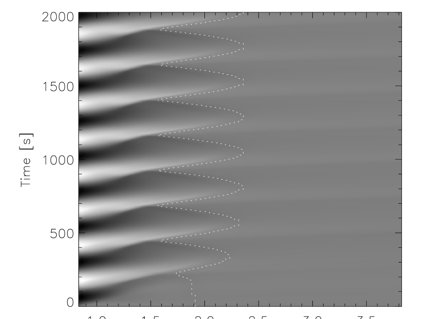
Figure 2.— The vertical energy flux density of the waves in an example case ($45^{\circ}$ inclination, 240 s driver period and 1100 m s^-1 initial amplitude). We have plotted the square root of the actual energy flux density in order to preserve the sign of the velocity — white represents upward velocity and black downward. Most of the energy ends up in standing waves in the chromosphere, while only a small fraction (almost invisible in this plot) reaches the corona. The dotted line is at the height where the temperature is 100 000 K, i.e. the lower transition region.

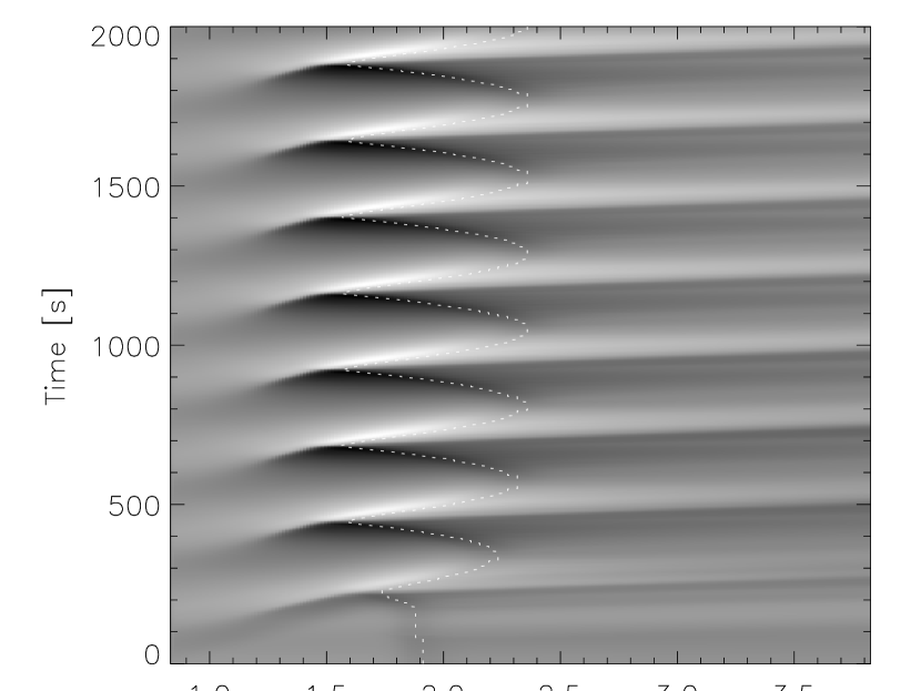
Figure 3.— The vertical velocity taken directly from the simulation data in the same case as Fig. 2. In addition to the main fronts and the parabolic shapes, we see an initial (quite weak) fast mode front and some additional fronts that seem to be generated at the tops of the fibrils. Again, the dotted line marks where T=100 000 K.

3. Analysis

In their observational study, Hansteen et al. (2006) and De Pontieu et al. (2007) find that fibrils, which they observe in H$\alpha$, follow parabolic paths in distance-time diagrams. These parabolic paths are found in our simulations as well, cf. Fig. 3. They can be visualized in a way more comparable to De Pontieu et al. if we instead show the temperature in a distance-time plot, as in Fig. 4. We clearly see the parabolic paths traced by the transition region as it is periodically pushed up by the passing shock waves. H$\alpha$ radiation is primarily generated in the hot upper layers of the chromosphere just below the transition region, and observations in that band will therefore show very similar movement.

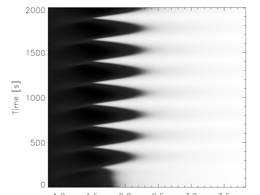
Figure 4.— The gas temperature as a function of time and vertical position in the same case as for Fig. 3. This way of plotting very clearly shows the movement of the transition region which is our primary interest.

A look at Fig. 3 tells us that, although the parabolic shapes are clearly seen, there are also other features present. Some fast mode waves remain — one can be seen faintly at the beginning of the simulation, before the first slow shock front — and some additional slow mode waves are apparently generated in the shock fronts through nonlinear processes. Although these other waves can have significant amplitudes, their effect on the movement of the transition region is far less than that of the slow mode shock waves. In addition, fast modes would tend to refract downwards in a real atmosphere, as discussed in the previous section.

The picture is clearer when looking at the temperature plot. Therefore, it seems reasonable to use the movement of the transition region as a proxy for the movement of the layers where the main H$\alpha$ radiation takes place, make parabolic fits of the position, and use derivatives of these to determine velocities and decelerations. This is similar to the method used by De Pontieu et al. (2007), and makes comparisons easier. Furthermore, it means that the calculated decelerations will be constants. An example of the parabolic fits is shown in Fig. 5.

Figure 5.— An example of the parabolic fitting process, for the same case as Figs. 3 and 4. The transition region height is defined as the height where the temperature is 100 000 K.

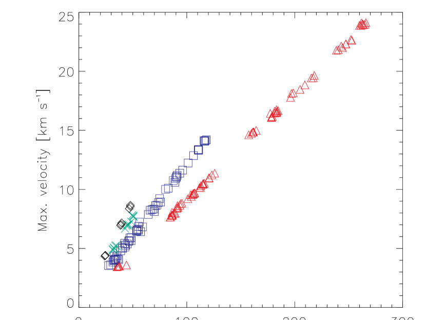
Figure 6.— Scatter plot of the maximum (upward or downward) velocities of fibrils vs. their decelerations, showing clear linear correlations. Red triangles correspond to a period of 180 s, blue squares to 240 s, green crosses to 300 s and black diamonds to 360 s. The slopes are clearly different as the period increases.

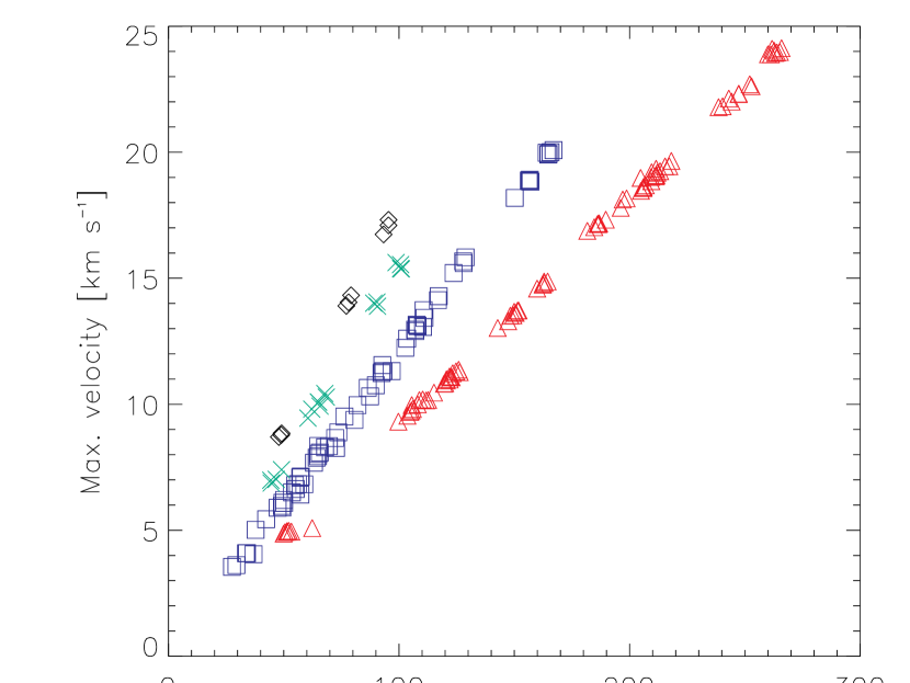
Figure 7.— As Fig. 6, but adjusted for projection effects.

Having determined the decelerations and velocities of each fibril from our 64 simulated cases (not all of which lead to noticeable movement of the transition region), a total of 190 fibrils, we can make scatterplots in the same way as De Pontieu et al. The results are shown in Figs. 6 and 7 — the latter is corrected for projection effects through multiplication by 1/cos $\theta$ when the field is inclined. We see obvious linear correlations between deceleration and maximum velocity, but the slopes are clearly different in the 180 s and 240 s cases. Although the number of points for the 300 s and 360 s cases is small, they too appear to show the same trend, giving progressively lower decelerations for a given maximum velocity. The data of De Pontieu et al. are much more scattered, both because of the greater difficulty in analysing multi-dimensional observational data and because of uncertainty in the relative orientations of the fibrils’ movement and the line of sight, but they also find a more or less linear correlation and signs of a period-dependent slope — again giving smaller decelerations at greater periods.

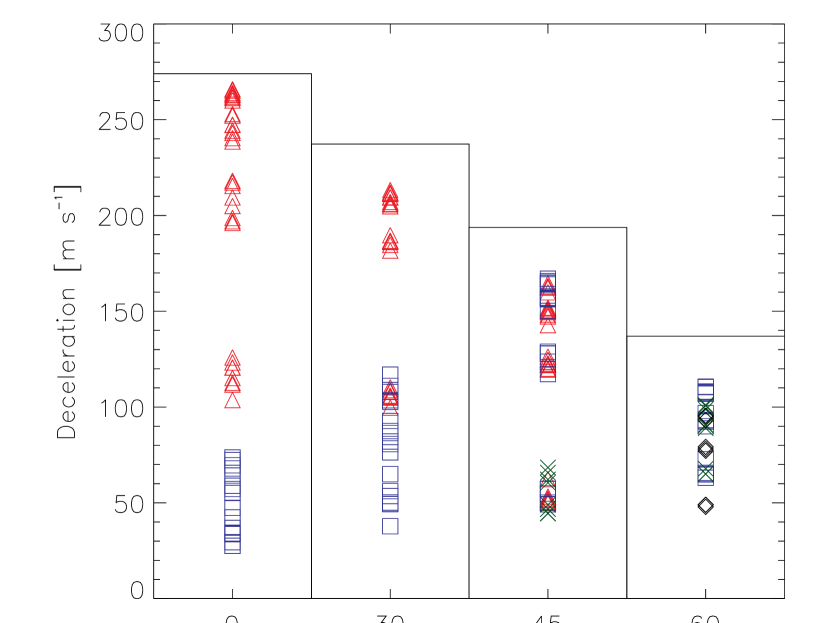
Figure 8.— Distribution of decelerations with magnetic field inclination. The data symbols are the same as in Fig. 6. All decelerations are lower than the projected gravity (solid columns), often very much lower. Since we have already compensated for projection effects, this distribution is extremely hard to reconcile with a ballistic theory.

A question of interest is how big a role gravity plays in setting the deceleration. One natural instinct when seeing the parabolic paths is to assume that we are observing a ballistic flight under the influence of solar gravity, with differences being accounted for by inclination and line of sight effects. In observations, the angle between the fibril movement and the line of sight is often difficult to determine exactly, but the many low decelerations reported would require extremely steep inclinations for the fibrils (Suematsu et al., 1995; De Pontieu et al., 2007).

In looking at our simulation data, we have no line of sight uncertainty, and compensating for the inclination of the fibrils is trivial. We can therefore easily calculate the distribution of decelerations with inclination angle. This distribution is shown in Fig. 8. The black histogram shows the field-aligned component of the solar gravitational acceleration, while the data points are shown with the same shapes and colour scheme as used in Fig. 6. We see that all our observed decelerations are smaller than the projected gravity, and often significantly smaller. Furthermore, they are not particularly clustered, pretty much the whole range of decelerations from about 50 m s^-1 to gravity being represented at all angles. With all projection effects already accounted for, this distribution is extremely hard to reconcile with a ballistic model, and indicates that we should look not to gravity but elsewhere in trying to explain it.

One alternative is to look at shock wave physics and pressure forces. The period of a wave train should remain constant during its propagation, and in that case, a fully developed shock wave (an N-wave) has a given time during which the amplitude must move from its highest to its lowest value. If the maximum amplitude — approximately the same magnitude as the maximum velocity of the fibril — increases, the deceleration must then be greater per unit time. Similarly, if the period is longer, the wave has more time between maximum and minimum amplitude, and the slope becomes less steep, meaning the deceleration is lower for a given amplitude. This is illustrated in Fig. 9.

Figure 9.— An N-wave with lower amplitude (dotted line) will have a less steep descending slope (lower deceleration) than one with higher amplitude (solid line) at a given period. Similarly, one with a longer period (dashed line) will have a lower deceleration than one with a shorter period at a given amplitude.

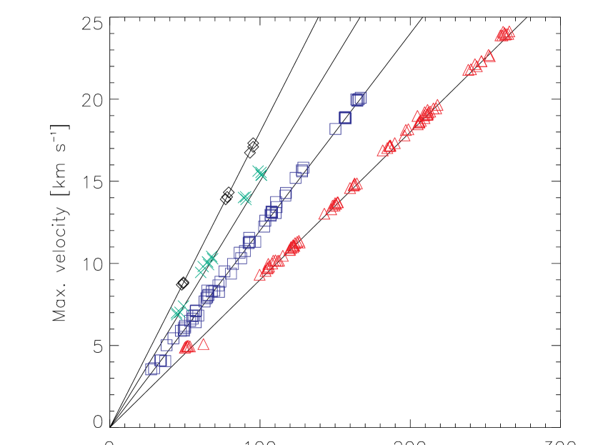
Figure 10.— As Fig. 7, but including the theoretical values from the shock deceleration hypothesis as solid lines. There is a near-perfect fit with the data, giving strong support to the hypothesis.

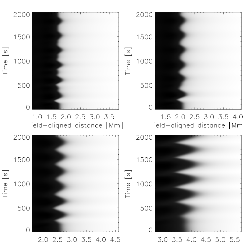
Figure 11.— Temperature plots showing the movement of the transition region with time. The period is 300 s; the piston amplitude is kept constant at 500 m s^-1, while the inclination of the magnetic field varies: $0^{\circ}$ (top left), $30^{\circ}$ (top right), $45^{\circ}$ (bottom left), $60^{\circ}$ (bottom right). As the inclination increases, the movement of the transition region becomes more regular and also gains in amplitude. The horizontal axis is distance along the field rather than height, in order to show the true length of the fibrils. The left boundary is at a different coordinate in each panel, so that the unperturbed transition region appears in the same position, but all panels are at the same scale.

The shock deceleration hypothesis can thus explain both the linear correlation between deceleration and maximum velocity and the variation in its slope with wave period. Indeed, we can calculate the decelerations expected from the theory as a function of period and maximum velocity/amplitude and compare them with the values from our simulations. The formula is simply

$$d=\frac{v_{max}}{P/2},$$ (1)

where $d$ is the deceleration, $v_{max}$ is the maximum velocity and $P$ the period of the wave. As we see in Fig. 10, there is near-perfect correspondence between the theoretical and simulated values, giving strong support to this explanation.

Although all the fibrils we study in this paper have decelerations below projected gravity, the shock wave deceleration model can also explain decelerations greater than gravity. Indeed, in preliminary experiments with even stronger piston driving we have produced decelerations that are slightly greater than gravity. Such decelerations have also recently been reported in observations of quiet sun mottles (Rouppe van der Voort et al., 2007).

One difference between our results and those of De Pontieu et al. (2007) is that they find many more fast fibrils than we do. Significant numbers have maximum velocities up to 25-30 km s^-1, whereas we only find such values for short-period waves propagating vertically. In fact, there are few fibrils with greater than 20 km s^-1 maximum velocity in our simulations. It is also worth noting that the data of De Pontieu et al. are not corrected for projection effects. We will touch on a possible explanation for this discrepancy later in this section.

We also find fibrils with lower maximum velocity than the lowest found in the observations. This is probably because the fibrils are quite easy to find and isolate in our simulation data, while superposition effects and background noise make small disturbances hard to detect in observations. These fibrils show a clear correspondence with the wave movement in the simulations, so they are not an effect of background noise there.

We now turn our attention to the question of whether the inclination of the field helps long-period waves propagate and reach coronal heights. Michalitsanos (1973) and Bel & Leroy (1977) made early investigations into this phenomenon. The idea is that if the plasma is confined to moving along the magnetic field, it will also be subjected to a reduced effective gravity $g\cos\theta$, where $\theta$ is the inclination of the magnetic field. With the acoustic cutoff period given as

$$P_{ac}=\frac{4\pi c_{s}}{\gamma g},$$ (2)

where $\gamma$ is the ratio of specific heats and $c_{s}$ the sound speed, a reduced effective gravity also leads to a higher cutoff period, thus allowing longer-period waves to propagate. More recently, Suematsu (1990) and De Pontieu et al. (2004, 2005) have proposed that this mechanism may let solar p-modes, with a period of around 5 minutes, propagate through the chromosphere and provide the driving force for spicules and fibrils. These waves are usually evanescent, having periods above the acoustic cutoff. In our model atmosphere, the cutoff period at the lower boundary is 213 s at 0^∘ inclination, 245 s at 30^∘, 301 s at 45^∘, and 425 s at 60^∘. The real solar chromosphere should have values close to these.

Note that the reduced effective gravity hypothesis only works if the plasma is in fact confined to moving along the magnetic field, that is, in low-$\beta$ plasma. In our model this applies everywhere, but on the actual sun, where the main source of wave energy is the convection region and photosphere, we would only expect long-period waves to be able to propagate upwards from the photosphere with significant energy in areas where the magnetic field is strong enough to dominate over thermal pressure forces even at photospheric depths. This applies mainly in the vicinity of sunspots, active regions and network flux concentrations.

In Fig. 11 we have plotted the movement of the transition region with time for four different inclinations, with the other parameters — piston period and amplitude — constant. The period is 300 s, and waves with this period ought to be evanescent in a vertical field, being above the cutoff period of 213 s.

With a vertical field (top left), there is some tunneling of wave energy, but the movement is slight and somewhat irregular. As the inclination of the field increases to $30^{\circ}$ (top right), $45^{\circ}$ (bottom left) and $60^{\circ}$ (bottom right), there is a clear progression towards more regular parabolic movement, and the amplitude also increases markedly. These results clearly support the hypothesis of Suematsu (1990) and De Pontieu et al. (2004, 2005). They also support the claim by De Pontieu et al. (2007) that the regional differences in behaviour they observe are at least partially caused by the inclination of the magnetic field, allowing longer period waves (with corresponding lower fibril decelerations) to propagate in regions of inclined field.

Table 1Maximum velocities (km s^-1)

0∘ inclination
	Driver amplitude (km s-1)
Period (s)	00.2	00.5	00.8	01.1
180	10.6	18.7	22.2	24.0
240	$\cdots$	$\cdots$	6.2	8.4
300	$\cdots$	$\cdots$	$\cdots$	$\cdots$
360	$\cdots$	$\cdots$	$\cdots$	$\cdots$
30∘ inclination
180	9.9	17.1	18.7	19.2
240	$\cdots$	6.1	9.7	12.9
300	$\cdots$	$\cdots$	$\cdots$	$\cdots$
360	$\cdots$	$\cdots$	$\cdots$	$\cdots$
45∘ inclination
180	5.0	11.1	13.5	14.8
240	6.6	15.3	18.7	20.0
300	$\cdots$	$\cdots$	7.1	9.9
360	$\cdots$	$\cdots$	$\cdots$	$\cdots$
60∘ inclination
180	$\cdots$	$\cdots$	$\cdots$	$\cdots$
240	$\cdots$	8.0	11.2	13.2
300	$\cdots$	10.2	14.0	15.5
360	$\cdots$	8.8	14.1	17.1

Note. — The values are averaged maximum velocities for all fibrils with that driver period and amplitude, corrected for projection effects. At the missing points, the movement of the transition region is irregular or has very low amplitude (¡ 5 km s^-1).

In Table 1, we have listed the averaged maximum velocities of all fibrils at given magnetic field inclinations, driver amplitudes and periods. Unsurprisingly, at 0^∘ inclination, only 180 s waves produce proper shocks, although it is possible to produce regular movement of the transition region with 240 s waves if the driving piston is strong enough. There is of course a dependence of the maximum velocity on the driver amplitude, but it is not linear. The maximum velocity at 180 s period increases by only about 10% when the driver amplitude increases from 0.8 to 1.1 km s^-1, a pattern that is repeated for several other combinations of period and inclination. It also increases by only a factor of 2.4 when the amplitude increases by a factor of 5.5, from 0.2 to 1.1 km s^-1. This indicates that the waves are reaching a plateau where larger initial amplitudes just lead to increased dissipation.

The maximum velocity of 180 s waves decreases when the inclination increases. Since these waves are well below the acoustic cutoff, this can not be because they are becoming evanescent; instead, it is likely because of the increased effective travel distance when the field is inclined. At 60^∘ inclination, the effective distance to the transition region is twice as long. This leads to increased dissipative losses as the wave travels through the chromosphere. The effect is more pronounced at 180 s because short-period waves steepen into shocks sooner and therefore are more vulnerable to dissipation.

At the other periods, the maximum velocities increase as the acoustic cutoff period increases, becoming noticeable when the wave period is similar to the cutoff and significant when it is well below. At 60^∘ inclination, the 240 s waves drop in amplitude again, while those with longer periods are at their strongest.

It should be noted that field inclination is not the only possible way to increase the cutoff period. We see in equation 2 that we can also modify the sound speed, which is proportional to the square root of the temperature. Hence, in a locally hotter medium, we can get easier propagation of long-period waves. This mechanism may be unlikely to be enough on its own, as you need a temperature increase by a factor 2 to get the same cutoff increase as a field inclination of 45^∘, and a factor 4 to match 60^∘; however, the combination of the two mechanisms could be very effective. For example, in the real solar atmosphere, the field tends to be more vertical at lower heights but becomes more inclined higher up due to the natural expansion of flux tubes. It is then possible that a local temperature enhancement could increase the cutoff period in the lower layers while the field inclination takes over as the waves propagate upwards. Preliminary experiments using a simple model with vertical field up to about 1000 km and inclined fields above that indicate that such a configuration can also let long-period waves propagate.

It could also be a possible reason why, in our simulations, we see fewer fibrils with very high maximum velocities than De Pontieu et al. (2007). In our model, the field inclination is constant, leading to a large increase in effective travel distance at higher inclinations. In a more realistic model with the field inclination increasing gradually, it is possible that the waves travel more vertically through lower parts of the atmosphere before the field inclination increases, leading to shorter travel distances and less dissipation.

4. Summary

Our simulations have shown that, even with a simple 1D model, we are able to reproduce the main observed properties of dynamic fibrils. We get parabolic shapes and reproduce the range of decelerations and roughly the range of maximum velocities found by De Pontieu et al. (2007). We find that the slope of the correlation between maximum velocity and deceleration varies with the driver period, with lower decelerations at longer periods. The distribution of decelerations is incompatible with a ballistic model but fits very well with a shock wave deceleration model. Furthermore, we have shown that long-period waves can propagate and reach the transition region if they travel in a strong inclined field, as suggested by Michalitsanos (1973) and Bel & Leroy (1977), and that they can drive fibrils there as suggested by Suematsu (1990) and De Pontieu et al. (2004, 2005). The different slopes of the correlation and the leakage of long-period waves can account for the regional differences in the observations. Our results give strong support to the theory that jets such as dynamic fibrils and quiet sun mottles are driven by slow mode magnetoacoustic shocks in the chromosphere.

References

- Arnaud & Rothenflug (1985) Arnaud, M. & Rothenflug, R. 1985, A&AS, 60, 425
- Beckers (1968) Beckers, J. M. 1968, Sol. Phys., 3, 367
- Bel & Leroy (1977) Bel, N. & Leroy, B. 1977, A&A, 55, 239
- Bogdan et al. (2003) Bogdan, T. J., Carlsson, M., Hansteen, V. H., McMurry, A., Rosenthal, C. S., Johnson, M., Petty-Powell, S., Zita, E. J., Stein, R. F., McIntosh, S. W., & Nordlund, Å. 2003, ApJ, 599, 626
- Christopoulou et al. (2001) Christopoulou, E. B., Georgakilas, A. A., & Koutchmy, S. 2001, Sol. Phys., 199, 61
- De Pontieu et al. (2005) De Pontieu, B., Erdélyi, R., & De Moortel, I. 2005, ApJ, 624, L61
- De Pontieu et al. (2004) De Pontieu, B., Erdélyi, R., & James, S. P. 2004, Nature, 430, 536
- De Pontieu et al. (2007) De Pontieu, B., Hansteen, V. H., Rouppe van der Voort, L., van Noort, M., & Carlsson, M. 2007, ApJ, 655, 624
- Grossmann-Doerth & Schmidt (1992) Grossmann-Doerth, U. & Schmidt, W. 1992, A&A, 264, 236
- Hansteen (2005) Hansteen, V. H. 2005, in IAU Symposium, ed. A. V. Stepanov, E. E. Benevolenskaya, & A. G. Kosovichev, 385–386
- Hansteen et al. (2006) Hansteen, V. H., De Pontieu, B., Rouppe van der Voort, L., van Noort, M., & Carlsson, M. 2006, ApJ, 647, L73
- Heggland (2003) Heggland, L. 2003, Waves in the Chromosphere and Corona, Master Thesis (University of Oslo)
- Jefferies et al. (2006) Jefferies, S. M., McIntosh, S. W., Armstrong, J. D., Bogdan, T. J., Cacciani, A., & Fleck, B. 2006, ApJ, 648, L151
- Judge & Meisner (1994) Judge, P. G. & Meisner, R. 1994, in The Third Soho Workshop, Solar Dynamic Phenomena and Solar Wind Consequences, ed. J. J. Hunt (ESTEC, Noordwijk, the Netherlands: ESA SP-373), 67–71
- McIntosh & Jefferies (2006) McIntosh, S. W. & Jefferies, S. M. 2006, ApJ, 647, L77
- Michalitsanos (1973) Michalitsanos, A. G. 1973, Sol. Phys., 30, 47
- Osterbrock (1961) Osterbrock, D. E. 1961, ApJ, 134, 347
- Rouppe van der Voort et al. (2007) Rouppe van der Voort, L. H. M., De Pontieu, B., Hansteen, V. H., Carlsson, M., & van Noort, M. 2007, submitted to ApJL
- Shull & van Steenberg (1982) Shull, J. M. & van Steenberg, M. 1982, ApJS, 48, 95
- Sterling (2000) Sterling, A. C. 2000, Sol. Phys., 196, 79
- Suematsu (1990) Suematsu, Y. 1990, LNP Vol. 367: Progress of Seismology of the Sun and Stars, 367, 211
- Suematsu et al. (1995) Suematsu, Y., Wang, H., & Zirin, H. 1995, ApJ, 450, 411
- Tsiropoula et al. (1994) Tsiropoula, G., Alissandrakis, C. E., & Schmieder, B. 1994, A&A, 290, 285