Swift Observations of the Cooling Accretion Disk of XTE J1817$-$330

Abstract

The black hole candidate X-ray transient XTE J1817$-$330 was observed by the Swift satellite over 160 days of its 2006 outburst with the XRT and UVOT instruments. At the start of the observations, the XRT spectra show that the 0.6-10 keV emission is dominated by an optically thick, geometrically thin accretion disk with an inner disk temperature of $\sim 0.8$ keV, indicating that the source was in a high/soft state during the initial outburst phase. We tracked the source through its decline into the low/hard state with the accretion disk cooling to $\sim 0.2\,\mathrm{keV}$ and the inner disk radius consistent with the innermost stable circular orbit at all times. Furthermore, the X-ray luminosity roughly follows $L_{X}\propto T^{4}$ during the decline, consistent with a geometrically stable blackbody. These results are the strongest evidence yet obtained that accretion disks do not automatically recede after a state transition, down to accretion rates as low as $0.001L_{Edd}$. Meanwhile, the near-UV flux does not track the X-ray disk flux, and is well in excess of what is predicted if the near-UV emission is from viscous dissipation in the outer disk. The strong correlation between the hard X-ray flux and the near-UV flux, which scale as $L_{X}^{0.5}$, indicate that reprocessed emission is most likely the dominate contribution to the near-UV flux. We discuss our results within the context of accretion disks and the overall accretion flow geometry in accreting black holes.

1. Introduction

At high mass accretion rates (those corresponding to $L_{X}/L_{Edd.}\geq 0.1$, approximately), it is expected that standard geometrically-thin but optically thick accretion disks should drive accretion onto compact objects. Stellar-mass black holes with low-mass companion stars provide an excellent laboratory for the study of disks. Many of these systems are transient, and the dramatic flux variations and state changes can be understood as resulting from variations in the accretion rate. The timescales in such disks are readily accessible (the viscous timescale for the entire disk is on the order of weeks), and light from the accretion process should strongly dominate that from the companion star. Fits to X-ray spectra with thermal disk models reveal trends broadly consistent with $L\propto T^{4}$ at high accretion rates (e.g., Miller, Fabian, & Miller, 2004).

Although it has long been assumed that light from the accretion disk dominates the emission from infrared to soft X-rays in actively accreting stellar mass black holes, recent observations suggest that this may not always be the case. For instance, Homan et al. (2005) find that the infrared emission in the stellar-mass black hole GX 339$-$4 may be jet-based synchrotron radiation. In the stellar-mass black hole XTE J1118$+$480, Hynes et al. (2006) find that even the UV emission may be partially due to synchrotron emission. On the other hand, Russell et al. (2006) showed that the optical/near-infrared (NIR) emission from an ensemble of 33 black hole X-ray binaries (BHXRBs) is more consistent with reprocessed hard X-ray emission rather than synchrotron emission or direct observations of emission from the accretion disk.

It is also expected that accretion disks should be radially truncated at low mass accretion rates (corresponding to $L_{X}/L_{Edd.}\leq 0.01$), and replaced by an advection-dominated flow (Esin, McClintock, & Narayan, 1997). Recent analyses of GX 339$-$4, Cygnus X-1, and SWIFT J1753.5$-$0127 have revealed cool accretion disks that appear to remain close to the black hole at low accretion rates (Miller et al., 2006b, a). However, observations which strongly constrain the nature of radio to X-ray emission mechanisms and the nature of accretion disks in stellar-mass black holes are still relatively few.

Dense multi-wavelength sampling has proved to be very powerful in revealing the nature of accretion flows in compact objects. Some of the most productive studies have correlated X-ray and radio flux measurements in black holes, as a coarse probe of disk–jet coupling (see, e.g., Gallo et al., 2003; Merloni et al., 2005). New work has linked specific (perhaps disk–driven) timing signatures in X-ray power spectra with radio jet flux (Migliari, Fender, & van der Klis, 2005). The large number of contemporaneous X-ray and radio observations made during the outbursts of transient black holes has been central to this work, and has been greatly facilitated by the ability of Rossi X-ray Timing Explorer (RXTE) to make frequent observations.

The Swift Gamma-Ray Burst Explorer (Gehrels et al., 2004) is dedicated to the discovery and follow-up study of gamma-ray bursts. It also offers the extraordinary opportunity to perform new multi-wavelength studies of X-ray transients that can reveal the nature of accretion disks around compact objects and the relation between disks, hard X-ray coronae, and radio jets. Swift carries the X-ray Telescope (XRT, Burrows et al., 2005), an imaging CCD spectrometer that reaches down to 0.3 keV. This provides substantially improved coverage of thermal accretion disk spectra over RXTE, which has an effective lower energy bound of 3 keV. Moreover, the Swift optical/UV telescope (UVOT, Roming et al., 2005) is ideally suited to tracing inflow through the accretion disk (UV emission should lead X-ray emission in a standard thin accretion disk), and to testing the origin of near-ultraviolet (NUV) emission in accreting black holes.

XTE J1817$-$330 was discovered as a new bright X-ray transient with the RXTE All-sky monitor (ASM) on 2006 January 26 (Remillard et al., 2006). The ASM hardness ratios suggested a very soft source, making XTE J1817$-$330 a strong black hole candidate (e.g. White & Marshall, 1984). Initial pointed observations with RXTE confirmed the soft spectrum, and hinted at very low absorption along the line of sight (Miller et al., 2006c). A likely radio counterpart was detected on 2006 January 31 (Rupen et al., 2006), followed by the detection of counterparts at NIR, optical and ultraviolet wavelengths (D’Avanzo et al., 2006; Torres et al., 2006a; Steeghs et al., 2006). Pointed X-ray observations with Chandra confirmed that the absorption along the line of sight to XTE J1817$-$330 is very low (Miller et al., 2006d). The NUV apparent magnitude of XTE J1817$-$330 was comparable to the optical and infrared magnitudes, which further supports a low reddening towards the source.

The low absorption along the line of sight to XTE J1817$-$330 and its relatively simple fast-rise, exponential-decay (FRED) outburst profile made it an excellent source for intensive study with Swift. Through approximately 160 days of the 2006 outburst, Swift made a total of 21 snapshot observations in the NUV and X-ray bands. The resulting data represent the best sample of simultaneous NUV and X-ray follow-up observations yet obtained from a stellar-mass black hole evolving from the high/soft state to the low/hard state. Herein, we present an analysis of these simultaneous X-ray and NUV observations of XTE J1817$-$330. In Section 2, we detail the methods used to reduce and analyze the data. In Section 3, we present our analysis and results, including a re-analysis of Swift observations of GRO J1655$-$40. Our conclusions follow a brief summary in Section 4.

2. Observations and Data Reduction

Swift visited XTE J1817$-$330 on 21 occasions between 2006 February 18 and 2006 July 23. Tables 1 and 2 provide a journal of these observations. Figure 1 shows the RXTE/ASM light curve in the sum band (1.5-12 keV), with arrows indicating the dates of the Swift observations. XRT observations were taken in windowed timing (WT) mode while the transient was very bright, and in photon counting (PC) mode for the final four observations. The UVOT exposures were taken in six filters ($V$, $B$, $U$, $UVW1$, $UVW2$, $UVM2$) for the first three observations, and with the $UVW1$ filter subsequently. Table 2 provides the effective wavelengths for these filters.

Table 1XRT Observation Log

Obs.	Start	Exposure Time	Count Rate	Exclusion Box/Radius
Number	(UT)	(s)	($\mathrm{ct}\,\mathrm{s}^{-1}$)	(pixels)
001	2006 02 18 04:50:34	1105	776	15
002	2006 03 05 19:12:02	1467	544	10
	2006 03 06 17:57:47	530	532	10
003	2006 03 07 16:25:32	669	516	10
	2006 03 07 18:01:32	805	514	10
004	2006 03 15 07:26:31	1650	427	10
005	2006 03 15 16:59:36	1000	430	10
006	2006 04 08 11:25:05	835	266	5
007	2006 04 16 07:49:04	598	292	5
	2006 04 16 09:26:08	590	286	5
008	2006 04 24 00:20:08	890	259	5
009	2006 04 29 12:33:40	145	210	3
	2006 04 29 14:10:40	325	199	3
	2006 04 29 15:46:40	740	178	3
010	2006 05 09 16:41:46	975	165	3
011	2006 05 13 13:56:13	825	150	2
012	2006 05 20 19:24:02	955	120	2
013	2006 05 23 00:30:44	619	117	2
	2006 05 23 02:09:27	690	107	2
015	2006 06 04 07:50:45	560	77	0
	2006 06 04 09:27:45	375	77	0
016	2006 06 10 21:18:37	746	49	0
	2006 06 10 22:55:59	720	45	0
017	2006 06 18 17:24:44	684	24	0
	2006 06 18 19:03:40	560	25	0
018	2006 06 27 13:28:02	302	5	0
019	2006 07 02 15:34:23	519	1.8	3
	2006 07 02 17:11:23	455	1.9	3
020	2006 07 08 10:09:08	890	2.6	5
021	2006 07 16 17:11:50	434	1.59	3
	2006 07 16 18:46:37	440	1.55	3
022	2006 07 23 11:42:36	628	4.6	7
	2006 07 23 13:19:35	624	3.9	7

Table 2UVOT Observation Log and Photometry

Obs.	Start	Stop	Net Exp. Time	Filter	Mag.	$f_{\nu}$
	(UT)	(UT)	(s)			(mJy)
001	2006 02 18 04:50:39	04:53:42	183	$UVW2$	14.9(3)	1.0(3)
	2006 02 18 04:53:47	04:56:54	82	$V$	15.2(1)	2.5(2)
	2006 02 18 04:56:54	04:59:57	183	$UVM2$	15.0(1)	0.9(2)
	2006 02 18 05:00:03	05:03:11	102	$UVW1$	14.4(1)	1.7(1)
	2006 02 18 05:03:11	05:06:20	11	$U$	14.4(1)	2.3(2)
	2006 02 18 05:06:20	05:09:00	5	$B$	15.7(2)	1.9(4)
002	2006 03 05 19:12:07	18:04:35	881	$UVW2$	15.3(3)	0.7(2)
	2006 03 05 19:20:10	18:06:21	216	$V$	15.7(1)	1.7(1)
	2006 03 05 19:22:13	19:28:11	358	$UVM2$	15.4(1)	0.6(1)
	2006 03 05 19:28:17	19:32:16	235	$UVW1$	14.7(1)	1.2(1)
	2006 03 05 19:32:21	19:34:20	117	$U$	14.7(1)	1.8(1)
	2006 03 05 19:34:25	19:36:00	93	$B$	15.8(1)	1.8(2)
003	2006 03 07 16:25:37	18:06:04	515	$UVW2$	15.4(3)	0.7(2)
	2006 03 07 16:29:50	18:07:16	127	$V$	15.6(1)	1.8(1)
	2006 03 07 16:30:57	18:10:41	386	$UVM2$	15.4(1)	0.6(1)
	2006 03 07 16:34:08	18:13:01	253	$UVW1$	14.7(1)	1.2(1)
	2006 03 07 16:36:17	18:14:12	89	$U$	14.8(1)	1.6(1)
	2006 03 07 18:14:17	18:15:00	42	$B$	15.8(1)	1.9(2)
004	2006 03 15 07:26:36	07:54:01	1612	$UVW1$	14.9(1)	1.0(1)
005	2006 03 15 16:59:42	17:06:45	423	$UVW2$	15.5(3)	0.6(2)
	2006 03 15 17:06:50	17:13:53	416	$V$	15.7(1)	1.7(1)
	2006 03 15 17:13:59	17:16:16	136	$UVM2$	15.7(1)	0.5(1)
007	2006 04 16 07:49:08	09:36:00	1161	$UVW1$	15.2(1)	0.76(5)
008	2006 04 24 00:20:12	00:35:00	874	$UVW1$	15.4(1)	0.64(4)
009	2006 04 29 12:33:45	15:59:00	1167	$UVW1$	15.6(1)	0.55(4)
010	2006 05 09 16:41:51	16:58:00	954	$UVW1$	15.8(1)	0.43(3)
011	2006 05 13 13:56:18	14:10:00	809	$UVW1$	15.8(1)	0.43(3)
012	2006 05 20 19:24:07	19:40:00	938	$UVW1$	16.0(1)	0.38(3)
013	2006 05 23 00:30:50	02:21:00	1277	$UVW1$	16.1(1)	0.35(2)
016	2006 06 10 21:18:42	23:08:00	1390	$UVW1$	16.4(1)	0.26(2)
017	2006 06 18 19:03:45	19:13:01	547	$UVW1$	16.6(1)	0.22(2)
018	2006 06 27 13:28:07	16:51:00	874	$UVW1$	16.9(1)	0.17(1)
019	2006 07 02 15:34:28	17:19:01	950	$UVW1$	17.1(1)	0.13(1)
020	2006 07 08 10:09:13	10:24:00	873	$UVW1$	17.1(1)	0.14(1)
021	2006 07 16 17:11:55	18:54:00	850	$UVW1$	17.1(1)	0.13(1)
022	2006 07 23 11:42:42	13:30:00	1219	$UVW1$	17.1(1)	0.14(1)

Figure 1.— RXTE/ASM light curve of the 2006 outburst of XTE J1817$-$330. The count rates are daily averages in the sum (1.5-12 keV) band. The arrows denote the dates of the Swift observations, as described in Table 1.

2.1. XRT Data Reduction

The XRT observations were processed using the packages and tools available in HEASOFT version 6.1. Initial event cleaning was performed with “xrtpipeline” using standard quality cuts, and event grades 0-2 in WT mode (0-12 in PC mode). For the WT mode data, source extraction was performed with “xselect” in a rectangular box 20 pixels wide and 60 pixels long. Background extraction was performed with a box 20 pixels wide and 60 pixel long far from the source region. Several Swift observations in WT mode contain multiple pointings separated by a few hours. For these observations, each individual pointing was processed separately, as the detector response varies depending on the location of the source in the field of view. For the PC mode data, source extraction was performed with a 30 pixel radius circular aperture, and background extraction was performed with an annulus with an inner (outer) radius of 50 (100) pixels. The PC mode observations with multiple pointings were combined, in spite of the slight variation in the spectral response, to increase the signal-to-noise due to the faintness of the source.

After event selection, exposure maps were generated with “xrtexpomap”, and ancillary response function (arf) files with “xrtmkarf”. The latest response files (v008) were used from the CALDB database. All spectra considered in this paper were grouped to require at least 20 counts per bin using the ftool “grppha” to ensure valid results using $\chi^{2}$ statistical analysis. The spectra were analyzed using XSPEC version 11.3.2 (Arnaud, 1996). Fits made with the WT mode data were restricted to the 0.6-10 keV range due to calibration uncertainties at energies less than 0.6 keV. Similarly, fits to the PC mode data were restricted to the 0.3-10 keV range. All of the X-ray flux measurements, unless otherwise noted, are in the 0.6-10 keV range. The uncertainties reported in this work are 90% confidence errors, obtained by allowing all fit parameters to vary simultaneously.

The WT observations were strongly affected by pile-up, especially in the early observations when the raw uncorrected count rate was as large as $775\,\mathrm{ct}\,\mathrm{s}^{-1}$ (0.6-10 keV). When the observations suffer from pile-up, multiple soft photons can be observed at nearly the same time, and appear as a single hard photon. This creates an artificial deficit of soft photons and an excess of hard photons, and thus hardens the resulting spectral fit. To correct for pile-up, we followed the spectral fitting method described in Romano et al. (2006): we used various exclusion regions at the center of the source and re-fit the continuum spectrum (see below) with each exclusion region. When changing the exclusion region did not vary the fit parameters significantly ($<1\sigma$) we had properly corrected for pile-up. The sizes of the exclusion regions used are listed in Table 1. They are consistent with or larger than those used in Romano et al. (2006).

2.2. UVOT Data Reduction

The UVOT images were initially processed at HEASARC using the standard Swift “uvotpipeline” procedure, with standard event cleaning. The initial astrometric solution of UVOT images is typically offset by 5-10”. We corrected for this offset by matching the detected stars with the USNO B1.0 catalog, improving the aspect solution to better than 1”. After this correction, we stacked the images in observations with more than one exposure with the “uvotimsum” procedure.

The UVOT images were very crowded due to the low Galactic latitude ($-8.0^{\circ}$) and relatively low absorption in the line of sight. This presented a number of challenges in obtaining an absolute flux calibration for the NUV images, and we could not use the standard UVOT analysis procedure. Initial photometry was performed using “uvotdetect” and “uvotmag”. The first program, “uvotdetect”, runs SExtractor (Bertin & Arnouts, 1996) to extract sources and to calculate uncorrected count rates in a fixed aperture. SExtractor provides robust background estimations which are useful for this crowded field where it is difficult to find a source-free background annulus. The second program, “uvotmag”, corrects for coincidence loss and converts count rates to magnitudes using the photometric zero-points determined in orbit. The zero-points were determined with a 12 pixel ($6\arcsec$) radius aperture for the optical filters ($U$, $B$, $V$) and a 24 pixel ($12\arcsec$) radius aperture for the NUV filters ($UVW1$, $UVW2$, $UVM2$). The counterpart to XTE J1817$-$330 was sufficiently isolated from neighboring stars, and we were able to use a 12 pixel radius aperture to perform aperture photometry in all filters. The large aperture sacrifices some signal-to-noise in exchange for proper coincidence loss correction in the initial observations when the counterpart is very bright. In addition, this aperture is matched to that used to obtain the photometric zero-points of the optical filters, thus avoiding the need for aperture corrections for these filters.

We were required to perform aperture correction on the images taken with the NUV filters to use the proper photometric zero-point, which was determined with a 24 pixel aperture. For this correction we chose 20 of the most isolated stars within $5\arcmin$ of the counterpart. The magnitudes of the comparison stars were calculated within 12/24 pixel apertures to calculate the median aperture correction. The RMS error for this correction was typically $5-10\%$. We also confirmed that the corrected light curves of the comparison stars were stable within $\sim 1\%$. The final magnitudes and flux densities are shown in Table 2. The quoted flux density errors include the errors in the photometric zero-points.

3. Analysis & Results

3.1. Column Density and Reddening

The Galactic column density and reddening in the direction of XTE J1817$-$330 is not well constrained. Miller et al. (2006d) obtained Chandra observations of XTE J1817$-$330 during the bright outburst, and found a low equivalent neutral hydrogen column density of $N_{H}=8.8-9.7\times 10^{20}\,\mathrm{cm}^{-2}$. This is smaller than that obtained from the Galactic HI map, which is $1.6\times 10^{21}\,\mathrm{cm}^{-2}$ (Dickey & Lockman, 1990), and implies a relatively short distance to XTE J1817$-$330. Torres et al. (2006b) obtained an optical spectrum during the early phase of the outburst and estimated the Galactic column density and reddening using the equivalent width (EW) of several interstellar bands. They find the Galactic column density to be between $1\times 10^{21}\,\mathrm{cm}^{-2}<N_{H}<3\times 10^{21}\,\mathrm{cm}^{-2}$, and the reddening between $0.1<E(B-V)<0.5$, depending on the calibration chosen. Given the uncertainties in the $E(B-V)/EW$ relationships for interstellar bands, we have chosen to use the Galactic column density $N_{H}$ to constrain the reddening in the direction of XTE J1817$-$330. In any case, the low column density and low reddening make XTE J1817$-$330 an advantageous target for both soft X-ray spectroscopy and NUV observations.

After fitting a number of XRT spectra with different continuum models, a value of $N_{H}=1.2\times 10^{21}\,\mathrm{cm}^{-2}$ was found to yield acceptable fits with the greatest frequency. Given that this value is broadly consistent with other values reported elsewhere, and given that a different choice of $N_{H}$ would only introduce an offset in the measured disk properties, and not a change in the trends reported in Section 3.2, $N_{H}=1.2\times 10^{21}\,\mathrm{cm}^{-2}$ was adopted throughout this work. This column density implies a reddening of $E(B-V)=0.215$, (Zombeck, 1990) which is also consistent with values reported elsewhere; similarly, varying $E(B-V)$ by $\sim 50\%$ does not change the trends described in Section 3.5.

3.2. XRT Spectral Analysis

We used XSPEC to make spectral fits for each individual XRT observation of XTE J1817$-$330. Observation 018 was not used because there were insufficient counts to constrain the spectrum. As previously mentioned, several WT mode observations contained multiple pointings which were processed separately. We fit these multiple pointings simultaneously, although we did not fix the relative normalizations, as the overall X-ray flux varied up to $\sim 10\%$ on timescales of less than a day. To constrain the properties of the cool disk, we have assumed that the column density to XTE J1817$-$330 does not vary with time, and it has been fixed at $N_{H}=1.2\times 10^{21}\,\mathrm{cm}^{-2}$ as described in the previous section.

The XRT spectra of XTE J1817$-$330 cannot be adequately fit with a continuum model with a single component. In the early observations, the soft disk emission dominates, but there is a significant hard excess. In the late observations, the hard X-ray emission dominates, but there is a significant soft excess over a simple power-law spectrum. To demonstrate that our conclusions about the disk emission do not depend on our assumptions about the origin of the hard X-ray emission we have fit the XRT spectra with two separate two-component absorbed models. In each case we start with a simple optically thick geometrically thin accretion disk with multiple blackbody components, as described in “diskbb” (Mitsuda et al., 1984). This is combined with (a) a simple power-law component or (b) a hot optically thin Comptonizing corona (Titarchuk, 1994). In all cases the two-component absorbed continuum model is sufficient to describe the spectra. In the final observations, when one would expect to see a relativistically broadened iron line around $\sim 5\,\mathrm{keV}$ (McClintock & Remillard, 2006) there are insufficient statistics to allow a significant constraint on this component.

The “diskbb” model is very simple in that it does not factor in relativistic effects or radiative transfer, nor does it specify a zero-torque condition at the inner boundary (see, e.g., Zimmerman et al., 2005). More sophisticated disk models have certainly been developed, but “diskbb” is well understood, and correction factors aiming to describe spectral hardening through radiative transfer are based on this model. Furthermore, more sophisticated models do not give statistically superior results. As we are primarily interested in trends rather than absolute values, we have therefore chosen to use the familiar “diskbb” model.

In the first model, we have combined an accretion disk with a power-law component, denoted “diskbb+po”. This power-law component is a purely phenomenological fit and could be from a compact jet, a corona, or reprocessed emission. The results from this fit are shown in Table 3. The best-fit $\chi^{2}$ per degree of freedom ($\nu$) are acceptable for each observation. Using this model we observe the accretion disk cools significantly over the course of the observations from $\sim 0.8\,\mathrm{keV}$ to $\sim 0.2\,\mathrm{keV}$. Figure 2 shows three sample XRT spectra from observation 01, when the accretion disk dominates the emission; observation 16, when the disk and power-law have roughly equal contributions; and observation 22, when the power-law component dominates. The accretion disk component is significant in all spectra, except in observation 21. This low count-rate dataset did not require a soft component to achieve a good fit, but at the same time a disk contribution similar to those of observations 20 and 22 is consistent with the data. Through all the observations the normalization of the disk component, which is proportional to the square of the inner disk radius, does not show a significant trend. The spectral index of the power-law component varies considerably, from 1.4–3.2, also with no significant trend. However, for most of the early observations the power-law spectral index is not well constrained as the soft disk flux dominates the emission.

Table 3XRT Spectral fits with “diskbb+po” model

Obs.	$kT$	Norm	$\Gamma$	Norm.	Flux	Disk Flux	$\chi^{2}/\nu$
	(keV)				($\mathrm{erg}\,\mathrm{cm}^{-2}\,\mathrm{s}^{-1}$)	($\mathrm{erg}\,\mathrm{cm}^{-2}\,\mathrm{s}^{-1}$)
01	0.83(1)	$4.6(2)\times 10^{3}$	2.0(2)	0.8(2)	$4.3(2)\times 10^{-8}$	$3.9(2)\times 10^{-8}$	632.8/513
02	0.768(4)	$3.7(1)\times 10^{3}$	1.4(3)	$0.13^{+0.09}_{-0.07}$	$2.38(9)\times 10^{-8}$	$2.26(5)\times 10^{-8}$	1190.4/953
		$3.4(1)\times 10^{3}$		$0.07^{+0.06}_{-0.04}$	$2.13(6)\times 10^{-8}$	$2.07(4)\times 10^{-8}$
03	0.746(4)	$3.8(1)\times 10^{3}$	1.6(6)	$0.10^{+0.09}_{-0.07}$	$2.10(8)\times 10^{-8}$	$2.03(5)\times 10^{-8}$	906.4/881
		$3.7(1)\times 10^{3}$		$0.10^{+0.09}_{-0.08}$	$2.02(8)\times 10^{-8}$	$1.95(5)\times 10^{-8}$
04	0.700(7)	$3.4(2)\times 10^{3}$	2.1(1)	0.6(1)	$1.61(8)\times 10^{-8}$	$1.39(7)\times 10^{-8}$	596.1/493
05	0.694(8)	$3.5(2)\times 10^{3}$	2.1(1)	0.6(1)	$1.61(9)\times 10^{-8}$	$1.39(8)\times 10^{-8}$	571.8/448
06	0.611(8)	$3.3(2)\times 10^{3}$	2.7(1)	0.42(7)	$8.6(5)\times 10^{-9}$	$7.4(5)\times 10^{-9}$	391.7/372
07	0.646(6)	$3.2(1)\times 10^{3}$	2.4(2)	0.19(5)	$9.7(4)\times 10^{-9}$	$9.1(4)\times 10^{-9}$	848.4/751
		$2.9(1)\times 10^{3}$		0.24(7)	$9.2(5)\times 10^{-9}$	$8.4(4)\times 10^{-9}$
08	0.61(1)	$2.7(2)\times 10^{3}$	2.8(2)	0.29(5)	$6.8(5)\times 10^{-9}$	$6.0(4)\times 10^{-9}$	449.8/337
09	0.611(5)	$3.5(2)\times 10^{3}$	2.7(1)	$0.31^{+0.12}_{-0.06}$	$8.6(6)\times 10^{-9}$	$7.8(4)\times 10^{-9}$	1051.7/941
		$3.7(2)\times 10^{3}$		0.33(8)	$9.2(4)\times 10^{-9}$	$8.3(4)\times 10^{-9}$
		$4.2(2)\times 10^{3}$		$0.41^{+0.03}_{-0.06}$	$1.05(4)\times 10^{-8}$	$9.4(4)\times 10^{-9}$
10	0.532(8)	$4.3(3)\times 10^{3}$	3.0(2)	0.32(5)	$6.0(4)\times 10^{-9}$	$5.2(4)\times 10^{-9}$	419.2/329
11	0.529(7)	$3.4(2)\times 10^{3}$	2.8(2)	0.17(4)	$4.4(3)\times 10^{-9}$	$4.0(3)\times 10^{-9}$	418.6/322
12	0.495(7)	$3.7(3)\times 10^{3}$	3.2(2)	0.20(3)	$3.7(2)\times 10^{-9}$	$3.2(2)\times 10^{-9}$	334.3/287
13	0.480(7)	$3.3(3)\times 10^{3}$	3.1(1)	0.22(5)	$3.0(2)\times 10^{-9}$	$2.5(2)\times 10^{-9}$	550.6/473
		$3.5(3)\times 10^{3}$		0.20(3)	$3.1(2)\times 10^{-9}$	$2.6(2)\times 10^{-9}$
15	0.415(7)	$3.3(4)\times 10^{3}$	2.5(1)	0.28(3)	$2.2(2)\times 10^{-9}$	$1.3(1)\times 10^{-9}$	531.8/544
		$3.2(4)\times 10^{3}$		0.30(4)	$2.2(2)\times 10^{-9}$	$1.3(2)\times 10^{-9}$
16	0.293(6)	$8(1)\times 10^{3}$	2.4(1)	0.27(3)	$1.4(1)\times 10^{-9}$	$5.6(1)\times 10^{-10}$	544.7/563
		$7(1)\times 10^{3}$		0.27(3)	$1.3(1)\times 10^{-9}$	$4.8(1)\times 10^{-10}$
17	0.21(1)	$2.3(4)\times 10^{4}$	2.3(1)	0.14(1)	$7.3(7)\times 10^{-10}$	$2.4(5)\times 10^{-10}$	436.4/415
		$2.3(5)\times 10^{4}$		0.15(2)	$7.6(7)\times 10^{-10}$	$2.5(6)\times 10^{-10}$
19	0.2(1)	$6^{+27}_{-5}\times 10^{2}$	1.7(3)	$8(2)\times 10^{-3}$	$5(1)\times 10^{-11}$	$2.7^{+12}_{-2.5}\times 10^{-12}$	13.3/23
20	0.19(4)	$3^{+5}_{-1}\times 10^{3}$	1.5(3)	0.010(4)	$9(3)\times 10^{-11}$	$1.8^{+3.2}_{-1.0}\times 10^{-11}$	28.3/25
21			2.3(2)	0.012(1)	$4.4(4)\times 10^{-11}$		19.3/20
22	0.20(3)	$4^{+4}_{-2}\times 10^{3}$	2.1(3)	0.024(9)	$1.3(5)\times 10^{-10}$	$3.2^{+3.1}_{-1.8}\times 10^{-11}$	35.0/37

Note. — XRT spectral fits with a continuum model consisting of an optically thick geometrically thin accretion disk combined with a power-law component. This model, “diskbb+po”, is described in Section 3.2. Observations 1-17 have been fit from 0.6-10 keV, and observations 19-22 have been fit from 0.3-10 keV.

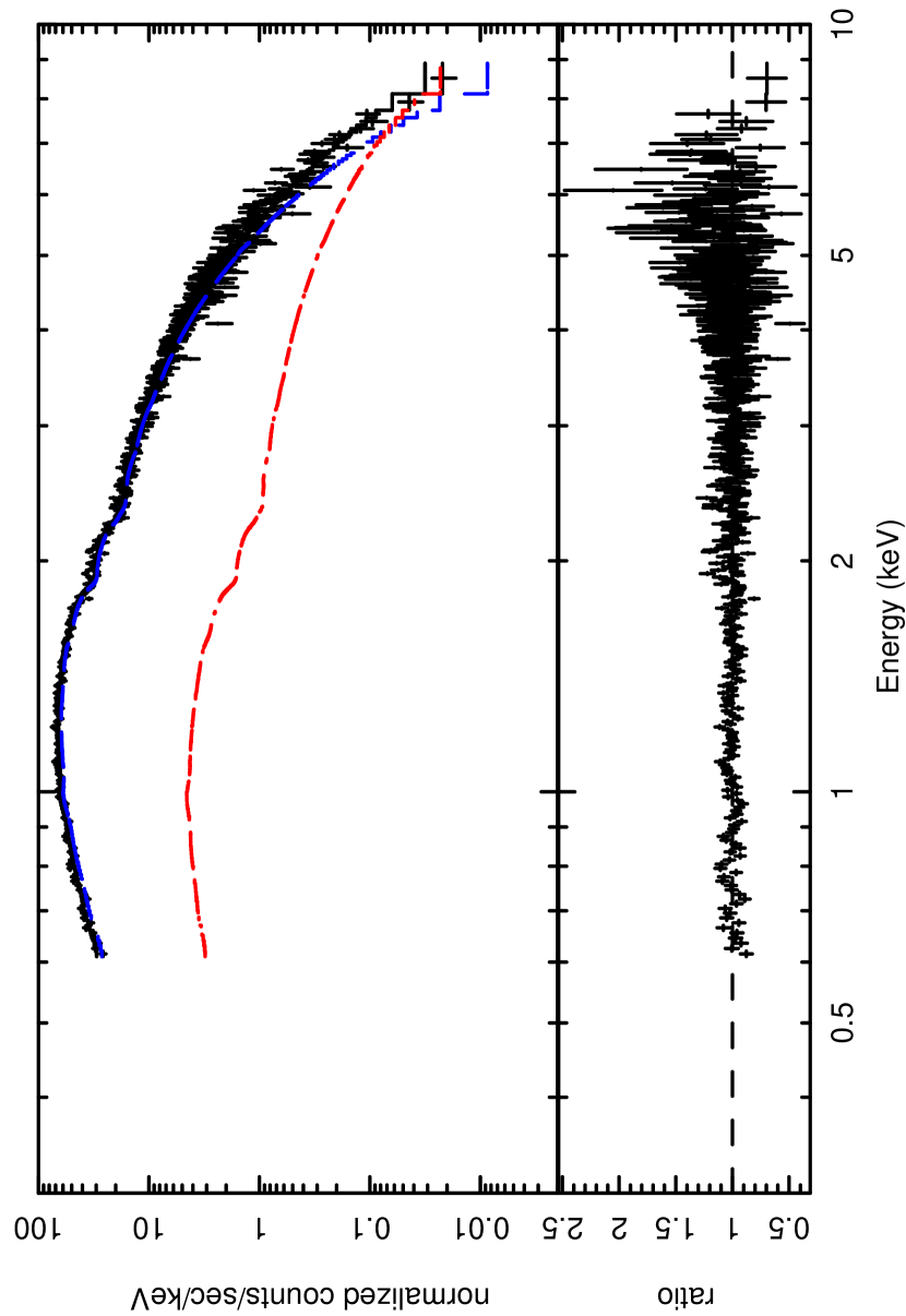
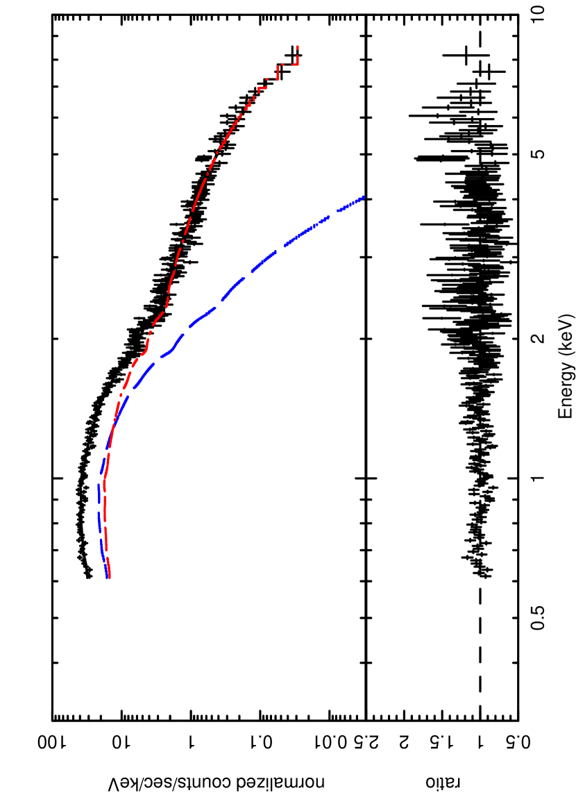
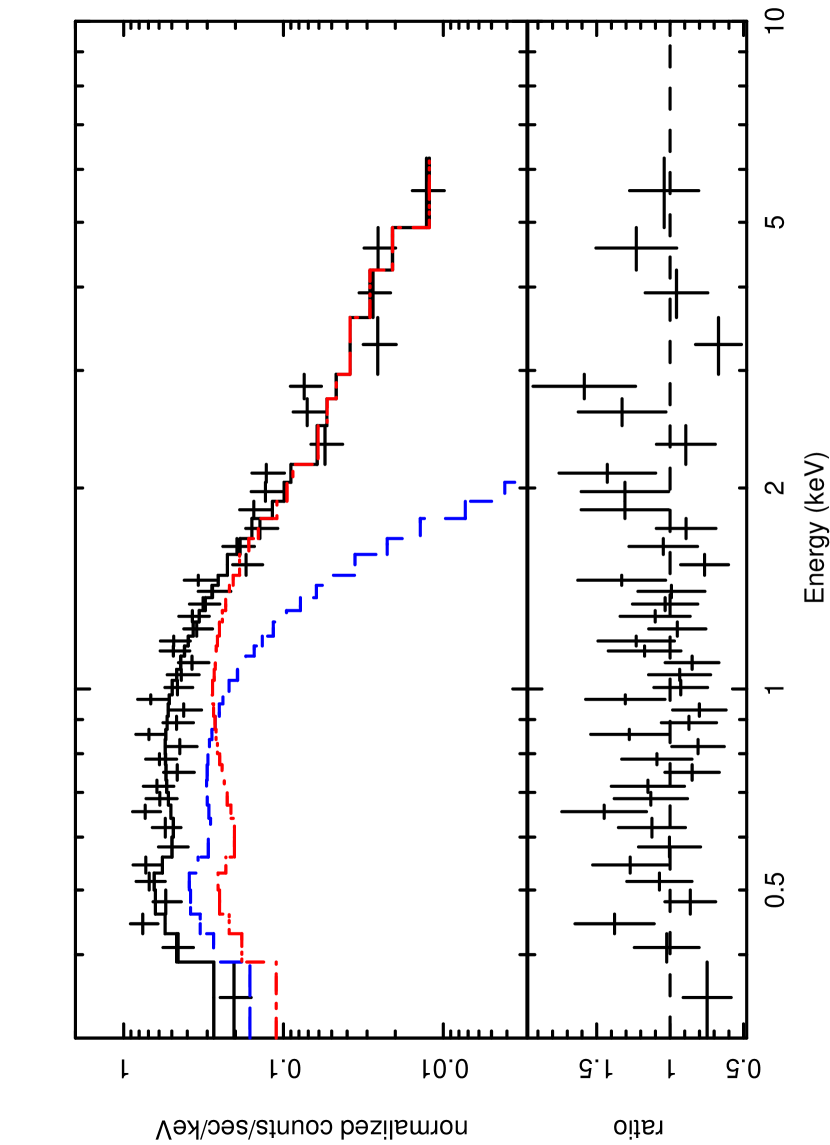
Figure 2.— Three XRT spectra of XTE J1817$-$330fit with an absorbed optically thick, geometrically thin accretion disk, with the addition of a power-law component, denoted “diskbb+po” in the text. The accretion disk component is colored blue, and the power-law component is colored red. The top panel shows the spectrum from observation 01, when the accretion disk dominates the emission. The middle panel shows observation 16, when the disk and power-law have roughly equal contributions. The bottom panel shows observation 22 when the power-law component dominates. There is clear evidence for both components in all three spectra.

In the second model, we have combined an accretion disk with a hot optically thin Comptonizing corona (Titarchuk, 1994), denoted “diskbb+comptt”. The electron temperature of the Comptonizing corona was fixed at 50 keV, and the seed photons were constrained to have the same temperature as the accretion disk. The results from this fit are shown in Table 4. The best-fit optical depth ($\tau$) of the Comptonizing corona is quite low, and for many observations we could only obtain an upper limit on $\tau$. Similar to our fits with the previous model, we were unable to fit the Comptonized model to observation 21, as we could not obtain a significant constraint on the accretion disk to provide seed photons for the hard component. As above, the best-fit values of $\chi^{2}/\nu$ are acceptable for each observation, and we see the accretion disk cooling with no significant trend in the accretion disk normalization parameter and inner disk radius.

Table 4XRT spectral fits with “diskbb+comptt” model

Obs.	$kT$	Norm	$kT_{e}$	$\tau$	Norm.	Flux	Disk Flux	$\chi^{2}/\nu$
	(keV)		(keV)			($\mathrm{erg}\,\mathrm{cm}^{-2}\,\mathrm{s}^{-1}$)	($\mathrm{erg}\,\mathrm{cm}^{-2}\,\mathrm{s}^{-1}$)
01	0.71(6)	$8(1)\times 10^{3}$	50.0	$<3.4\times 10^{-2}$	0.05(2)	$4.3(8)\times 10{-8}$	$3.4(6)\times 10^{-8}$	626.9/513
02	0.74(3)	$4.3(4)\times 10^{3}$		$0.12^{+0.3}_{-0.09}$	$9^{+6}_{-3}\times 10^{-3}$	$2.4(3)\times 10^{-8}$	$2.2(2)\times 10^{-8}$	1173.6/953
		$3.9(4)\times 10^{3}$	50.0		$5^{+5}_{-2}\times 10^{-3}$	$2.1(2)\times 10^{-8}$	$2.0(2)\times 10^{-8}$
03	0.72(3)	$4.4(5)\times 10^{3}$	50.0	$<0.4$	$7^{+6}_{-4}\times 10^{-3}$	$2.1(3)\times 10^{-8}$	$2.0(2)\times 10^{-8}$	899.8/881
		$4.2(5)\times 10^{3}$			$6^{+6}_{-4}\times 10^{-3}$	$2.0(3)\times 10^{-8}$	$1.9(2)\times 10^{-8}$
04	0.58(5)	$7(2)\times 10^{3}$	50.0	$0.03(2)$	$3(2)\times 10^{-2}$	$1.6(4)\times 10^{-8}$	$1.2(3)\times 10^{-8}$	576/493
05	0.56(5)	$8(2)\times 10^{3}$	50.0	$0.03^{+0.03}_{-0.01}$	$0.03(1)$	$1.6(4)\times 10^{-8}$	$1.1(3)\times 10^{-8}$	571.8/448
06	0.51(3)	$7(1)\times 10^{3}$	50.0	$<0.02$	$0.013(6)$	$9(1)\times 10^{-9}$	$7(1)\times 10^{-9}$	419.4/372
07	0.60(2)	$4.3(4)\times 10^{3}$	50.0	$<0.02$	$6(2)\times 10^{-3}$	$9.7(9)\times 10^{-9}$	$8.6(9)\times 10^{-9}$	855.5/751
		$4.1(4)\times 10^{3}$			$6(2)\times 10^{-3}$	$9.1(9)\times 10^{-9}$	$8.1(7)\times 10^{-9}$
08	0.53(3)	$4.7(4)\times 10^{3}$	50.0	$<0.04$	$7(3)\times 10^{-3}$	$6.7(7)\times 10^{-9}$	$5.7(4)\times 10^{-9}$	476.4/337
09	0.54(1)	$5.6(5)\times 10^{3}$	50.0	$<0.02$	$8(2)\times 10^{-3}$	$8.5(7)\times 10^{-9}$	$7.3(6)\times 10^{-9}$	1090.7/941
		$6.0(4)\times 10^{3}$			$9(1)\times 10^{-3}$	$9.2(6)\times 10^{-9}$	$7.9(6)\times 10^{-9}$
		$6.8(5)\times 10^{3}$			$1.0(2)\times 10^{-2}$	$1.0(1)\times 10^{-8}$	$8.9(6)\times 10^{-9}$
10	0.46(1)	$7.6(6)\times 10^{3}$	50.0	$<0.02$	$7(2)\times 10^{-3}$	$5.9(4)\times 10^{-9}$	$5.0(4)\times 10^{-9}$	453.7/329
11	0.47(3)	$5(1)\times 10^{3}$	50.0	$<0.04$	$5^{+1}_{-3}\times 10^{-3}$	$4.4^{+0.2}_{-0.7}\times 10^{-9}$	$3.7^{+0.2}_{-0.6}\times 10^{-9}$	431.5/322
12	0.44(2)	$6.5(8)\times 10^{3}$	50.0	$<0.03$	$4(2)\times 10^{-3}$	$3.6^{+0.2}_{-0.5}\times 10^{-9}$	$3.2^{+0.2}_{-0.4}\times 10^{-9}$	369.3/287
13	0.41(2)	$7(1)\times 10^{3}$	50.0	$<0.02$	$5(2)\times 10^{-3}$	$3.0^{+0.5}_{-0.2}\times 10^{-9}$	$2.4^{+0.4}_{-0.2}\times 10^{-9}$	575.4/473
		$7(1)\times 10^{3}$			$5(2)\times 10^{-3}$	$3.1^{+0.5}_{-0.2}\times 10^{-9}$	$2.5^{0.4}_{-0.2}\times 10^{-9}$
15	0.33(2)	$1.0(2)\times 10^{4}$	50.0	0.14(5)	$7(2)\times 10^{-3}$	$2.2(3)\times 10^{-9}$	$1.3(3)\times 10^{-9}$	554.1/544
		$1.0(2)\times 10^{4}$			$8(2)\times 10^{-3}$	$2.2^{+0.4}_{-0.3}\times 10^{-9}$	$1.3^{+0.3}_{-0.2}\times 10^{-9}$
16	0.25(1)	$2.3(4)\times 10^{4}$	50.0	$0.27^{+0.05}_{-0.01}$	$8(1)\times 10^{-3}$	$1.4(2)\times 10^{-9}$	$6.8(9)\times 10^{-10}$	580.8/563
		$2.1(3)\times 10^{4}$			$7(1)\times 10^{-3}$	$1.3(1)\times 10^{-9}$	$6(1)\times 10^{-10}$
17	0.19(1)	$4(1)\times 10^{4}$	50.0	0.35(4)	$5.6(6)\times 10^{-3}$	$7.3(8)\times 10^{-10}$	$2.8(8)\times 10^{-10}$	445/419
		$4(1)\times 10^{4}$			$5.8(9)\times 10^{-3}$	$7.6(9)\times 10^{-10}$	$2.8(7)\times 10^{-10}$
19	0.16(7)	$1.4^{+66}_{-1.1}\times 10^{3}$	50.0	$1^{+0.8}_{-0.3}$	$4^{+7}_{-1}\times 10^{-4}$	$5.0^{+0.2}_{-1.2}\times 10^{-11}$	$3.7^{+17}_{-2.7}\times 10^{-12}$	13.8/24
20	0.18(4)	$4^{+7}_{-2}\times 10^{3}$	50.0	$1.3^{+1.5}_{-0.6}$	$6(2)\times 10^{-4}$	$9^{+5}_{-2}\times 10^{-11}$	$2^{+4}_{-1}\times 10^{-11}$	28.8/26
22	0.18(5)	$8^{+16}_{-4}\times 10^{3}$	50.0	$0.5(2)$	$1.1^{+1.1}_{-0.3}\times 10^{-3}$	$1.3^{+1.2}_{-0.3}\times 10^{-10}$	$4^{+7}_{-2}\times 10^{-11}$	34.3/37

Note. — XRT spectral fits with a continuum model consisting of an optically thick geometrically thin accretion disk combined with a hot optically thin Comptonizing corona. This model, “diskbb+comptt”, is described in Section 3.2. Observations 1-17 have been fit from 0.6-10 keV, and observations 19-22 have been fit from 0.3-10 keV.

Independent of our assumption for the continuum model, we see the accretion disk cools from $\sim 0.8\,\mathrm{keV}$ to $\sim 0.2\,\mathrm{keV}$. A key theoretical prediction for a stellar-mass black hole accreting below its Eddington limit is that $\dot{M}\propto T^{4}$ and hence $f_{\mathrm{disk}}\propto T^{4}$ (Frank, King, & Raine, 2002). Figure 3 shows the disk flux as a function of disk temperature ($kT$) for each of the assumed models. For the “diskbb+po” model $f_{\mathrm{disk}}\propto T^{4.3\pm 0.1}$, and for the “diskbb+comptt” model $f_{\mathrm{disk}}\propto T^{3.3\pm 0.1}$. In each case the disk flux-temperature relation is close to the predicted relation over three orders of magnitude. This is a further demonstration that the size of the thin accretion disk is not changing significantly as it cools. The observed $T^{4}$ scaling also gives one some confidence that the employed “diskbb” model is validated, since the data scales as expected for such a simple model.

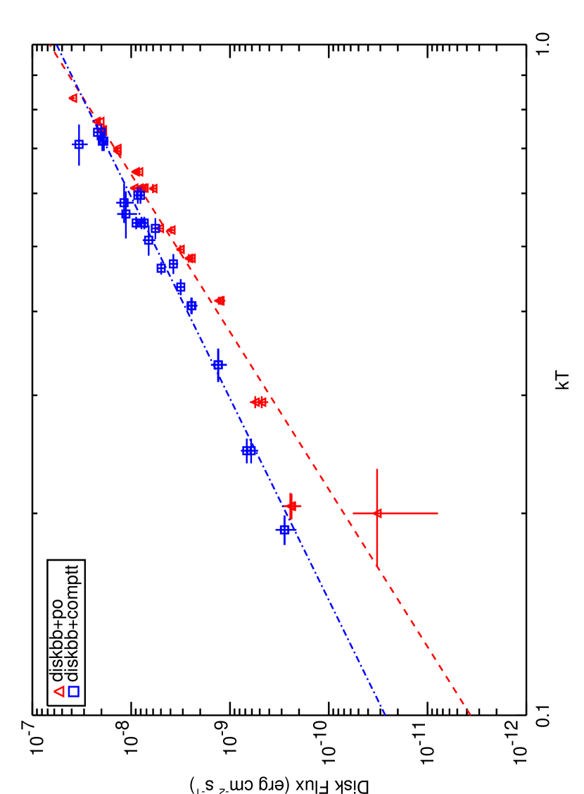
Figure 3.— Disk flux as a function of disk temperature for two different models. The triangles represent the flux and temperature values from the “diskbb+po” model, and the dashed line represents the best fit to these data. The squares represent the flux and temperature values from the “diskbb+comptt” model, and the dot-dashed line represents the best fit to these data. For the “diskbb+po” model $f_{\mathrm{disk}}\propto T^{4.3\pm 0.1}$, and for the “diskbb+comptt” model $f_{\mathrm{disk}}\propto T^{3.3\pm 0.1}$. In each case, for three orders of magnitude in flux the flux-temperature relation is very close to the predicted $f_{\mathrm{disk}}\propto T^{4}$.

3.3. X-ray and NUV Light Curve Comparison

We next investigated the relationship between the X-ray light curve and NUV light curve during the decline of the outburst of XTE J1817$-$330. The NUV light curve has been obtained in a single band, $UVW1$, with a peak response of 2600 Å. We have compared this to the X-ray flux values calculated with the “diskbb+po” model. Using the flux values from the “diskbb+comptt” model gives similar results. Figure 4-a shows the comparison of the total X-ray flux (black squares) to the $UVW1$ flux (magenta triangles) over the 160 days of observations. Each light curve has been normalized to a peak of 1.0 at the time of the first observation. Figure 4-b shows the comparison of the X-ray flux due to the disk component (blue x’s) to the $UVW1$ flux, and Figure 4-c shows the comparison of the X-ray flux due to the power-law component (red diamonds) to the $UVW1$ flux. It is readily apparent that the NUV flux most closely tracks the power-law flux in Figure 4-c and does not track the disk flux in Figure 4-b. The primary source of this difference is the $T^{4}$ scaling from above: the disk component of the X-ray flux declines very rapidly, which is not apparent in the NUV light curve. To mirror the X-ray variation, the NUV flux would have to fade by a factor of $\sim 250$ which we do not see at any time during our observations.

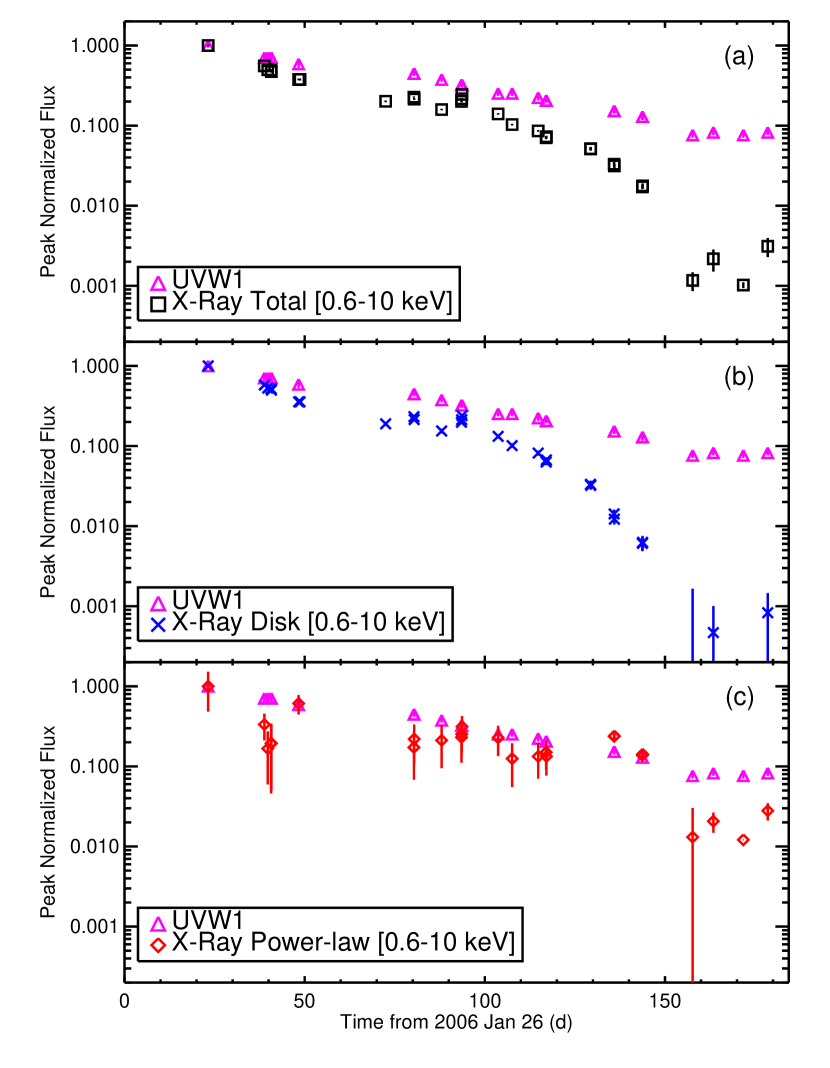
Figure 4.— Comparison of the NUV $UVW1$ and X-ray [0.6-10 keV] light curves over the 160 days of Swift observations. The top panel (a) shows the total X-ray flux (black squares) and the $UVW1$ flux (magenta triangles). The middle panel (b) shows the X-ray flux due to the disk component (blue x’s) and the $UVW1$ flux. The bottom panel (c) shows the X-ray flux due to the power-law component (red diamonds) and the $UVW1$ flux. In all cases the flux values have been normalized to a peak of 1.0 at the time of the first observation; the time scale on the X axis is relative to the outburst date of 2006 January 26. The NUV flux most closely tracks the X-ray power-law emission, and does not track the total X-ray flux or the X-ray disk flux.

3.4. NUV Emission as Reprocessed X-Ray Emission

We next investigate whether the NUV light is consistent with hard X-ray emission reprocessed by the outer accretion disk. van Paradijs & McClintock (1994) show that under simple geometric assumptions reprocessed emission should be proportional to $L_{X}^{0.5}\,a$, where $a$ is the orbital separation of the system. Another possibility, as suggested by the simultaneous spectral fitting above, is that we see jet emission directly in the NUV. Russell et al. (2006) point out that if the optical/NIR (and by extension the NUV) spectrum is jet dominated then it should be flat from the radio regime through the optical, and $L_{\mathrm{Opt/NIR/NUV}}\propto L_{X}^{0.7}$. In a study of an ensemble of 33 BHXRBs observed over many orders of magnitude of X-ray luminosity, Russell et al. (2006) have shown that the optical/NIR emission is more consistent with the prediction of reprocessed hard X-ray emission. Our multiple observations of XTE J1817$-$330 during its decline from outburst allow us to trace this relationship for a single source over several orders of magnitude of the X-ray luminosity and the accretion rate.

Figure 5 shows the NUV flux ${\nu}f_{\nu}$ for the $UVW1$ filter vs. the hard (2-10 keV) X-ray flux. We see a very strong correlation, with a best-fit power-law index of $0.47\pm 0.03$, consistent with the hypothesis that the NUV emission is dominated by reprocessed hard X-ray emission. It is important to note that this relationship, which is independent of reddening in the direction of the source, holds over more than two orders of magnitude of X-ray flux. As shown above with the light curve comparisons, this relationship is not consistent with the NUV emission being dominated by direct emission from the thermal accretion disk.

Figure 5.— NUV flux vs. hard X-ray flux for XTE J1817$-$330. The $UVW1$ flux tracks closely with the hard (2-10 keV) X-ray emission. The best-fit slope is $0.47\pm 0.02$, consistent with the hypothesis that the NUV emission is reprocessed hard X-ray emission.

King & Ritter (1998) predicted that when the optical/NUV flux is dominated by reprocessed hard X-ray emission, the $e$-folding time of the optical/NUV light curve ($\tau_{NUV}$) should be roughly twice the $e$-folding time of the X-ray light curve ($\tau_{X}$), where the decay is roughly exponential: $f\sim f_{0}e^{-t/\tau}$. This relationship has been observed in several X-ray novae, with typical X-ray light curve decay timescales of $\sim 30\,\mathrm{d}$ (Chen et al., 1997). The hard X-ray decay constant of XTE J1817$-$330 is best measured with the densely sampled ASM light curve shown in Figure 1. Using the ASM data from 5 d to 150 d after the initial outburst, when the transient was no longer significantly detected in the 1-day averages, we find $\tau_{X}=30\pm 3\,\mathrm{d}$. This is consistent with the $e$-folding time measured from the XRT light curve in the hard (2-10 keV) band, which is $\tau_{X}\sim 35\,\mathrm{d}$. The NUV light curve, using the data from 23 d to 150 d after the outburst, is well fit with an $e$-folding time of $61\pm 2\,\mathrm{d}$; the $e$-folding time is not significantly different when using the entire NUV data set. Thus the ratio of $e$-folding times, $\tau_{NUV}/\tau_{X}\sim 1.7-2.0$, shows that the NUV emission is consistent with being dominated by reprocessed hard X-ray emission through the final Swift observation.

3.5. XRT and UVOT Simultaneous Spectral Analysis

In order to provide additional constraints on the nature of the NUV emission, we have performed simultaneous spectral fits with the XRT spectra and the UVOT images. Only the first three observations, when the disk flux dominated the X-ray emission, were obtained with six UVOT filters. For most of the other UVOT observations only the $UVW1$ filter was used, providing fewer constraints on the simultaneous spectral fits. However, even a single NUV band is sufficient to test whether or not the NUV emission might be an extrapolation of the X-ray disk emission or power-law emission. We illustrate these broadband fits with observation 01, when the accretion disk emission dominates the X-ray flux; observation 16, when the accretion disk and hard power-law have roughly equal contributions; and observation 22, when the power-law emission dominates.

The UVOT magnitudes were converted to XSPEC compatible files using a modified version of “uvot2pha”, and the latest UVOT spectral response files (v103). We fit the XRT and UVOT spectra using the accretion disk and power-law model (“diskbb+po”) described previously. We fix the equivalent hydrogen column density ($N_{H}$) and optical/NUV reddening with the Milky Way reddening law of Cardelli et al. (1989), as described in Section 3.1.

The results of three spectral fits to observation 01, 16, and 22 are shown in Table 5 and plotted in Figure 6. In all the observations, the NUV emission is well in excess of an extrapolation of the disk flux as seen in the X-rays. In the earliest observations the NUV emission is a factor of $\sim 3$ brighter than an extrapolation, and in the final observations the NUV is a factor of $\sim 20$ brighter. If the Galactic reddening is larger than we assumed, then this discrepancy is even larger. This is consistent with our observations of the NUV and X-ray light curves, where the X-ray disk flux fades much faster than the NUV flux.

Table 5X-ray and NUV simultaneous spectral fits

Obs.	$kT$	Norm	$\Gamma$	Norm.	$\chi^{2}/\nu$
	(keV)
01	0.82(1)	$5.0(2)\times 10^{3}$	1.49(3)	0.32(4)	682.2/519
16	0.32(1)	$7.9(6)\times 10^{3}$	1.55(2)	0.071(3)	442.4/283
22	0.21(2)	$4(2)\times 10^{3}$	1.73(3)	0.016(2)	36.5/37

Note. — XRT and UVOT simultaneous spectral fits with a continuum model consisting of an optically thick geometrically thin accretion disk combined with a power-law component. This model, “diskbb+po”, is described in Sections 3.2 and 3.5.

Figure 6.— Three simultaneous spectral fits to the XRT and UVOT observations of XTE J1817$-$330. The fit model is a reddened (in the NUV) and absorbed (in the X-rays) accretion disk plus an power-law component. The reddening index $E(B-V)$ has been fixed at 0.215 mag. The top panel shows the best fit spectrum of observation 01, when the accretion disk component dominates the soft X-ray emission. The UVOT emission is well in excess of an extrapolation of the disk component, and is roughly consistent with an extrapolation of the power-law emission. The NUV colors, which are not well constrained, appear a bit bluer than the power-law extrapolation predicts. The middle panel shows the spectrum of observation 16. Although the NUV emission is well fit by the power-law, there are large residuals in the X-ray spectrum. The bottom panel shows the spectrum of observation 22. In this instance the NUV emission is directly on the extrapolation of the best-fit power-law in the X-ray spectrum. In observation 22 an extrapolation of the accretion disk spectrum to the NUV provides negligible flux relative to the power-law.

The simultaneous spectral fits in Figure 6 show that the NUV excess can be adequately fit by extrapolating the hard power-law from the X-ray band to the NUV. This implies that the NUV light might be from the same emission region as the hard X-ray flux. However, there are some important caveats. First, the six UVOT colors in observation 01 are only marginally consistent with the power-law extrapolation; however, the de-reddened NUV spectral index is strongly depending on the value of $E(B-V)$ chosen, which is not well constrained. Second, in observation 16, where we have high signal-to-noise and a well constrained power-law in the X-rays (as shown in the middle panel of Figure 2), $\chi^{2}/\nu$ of the fit is rather poor, and significant structure is seen in the fit residuals of the middle panel of Figure 6. It seems that using the “diskbb+po” model for the simultaneous spectra is overly simplistic. Thus, the NUV emission, while clearly in excess of the disk emission, is more consistent with reprocessed hard X-ray emission than an extrapolation of the X-ray power-law to the NUV regime.

3.6. Comparison to GRO J1655-40

Recently, Brocksopp et al. (2006) obtained multiple epoch Swift observations of the 2005 outburst of GRO J1655$-$40. They observed this black hole X-ray transient to rise from the low/hard state to the high/soft state, and for a brief time in a very high state. The light curve morphology of the 2005 outburst of GRO J1655$-$40 was much more complicated than the simple FRED profile of the 2006 outburst of XTE J1817$-$330. However, the spectrum of the initial observation of GRO J1655$-$40 closely resembles the spectrum of the final observation of XTE J1817$-$330. Brocksopp et al. (2006) find that the (0.7-9.6 keV) X-ray spectrum in this observation is consistent with an absorbed power-law, with the addition of a low significance relativistically broadened iron line at $\sim 6.4\,\mathrm{keV}$.

We have re-analyzed the XRT observation (0003000902) of GRO J1655$-$40 in the low/hard state, to compare it directly to our results for XTE J1817$-$330. If we fit an absorbed power-law model without a fixed absorption column density, we are able to replicate the spectral fits from Brocksopp et al. (2006). However, the best-fit value of $N_{H}=(5.9\pm 0.2)\times 10^{21}\,\mathrm{cm}^{-2}$ is significantly lower than that obtained in the high-soft state ($N_{H}=6.6-7.8\times 10^{21}\,\mathrm{cm}^{-2}$). By allowing the column density to float, we are masking any contribution from a dim, soft accretion disk. Therefore, we have chosen to fix the column density at $6.66\times 10^{21}\,\mathrm{cm}^{-2}$, which was determined by multi-wavelength observations of the 1996 outburst of GRO J1655$-$40 (Hynes et al., 1998). This column density is consistent with the values determined during the subsequent Swift observations, and is also consistent with the value obtained from the Galactic HI map, $6.9\times 10^{21}\,\mathrm{cm}^{-2}$ (Dickey & Lockman, 1990).

We find there is a small but significant excess of soft emission. We first fit the spectrum with an absorbed power-law spectrum, with a fixed column density, and find a best fit $\chi^{2}/\nu=793.4/642$. After adding an accretion disk component, we significantly improve the fit with a new $\chi^{2}/\nu=730.4/640$. The F-test statistic for adding the extra model component is 27.6, with probability of $3.2\times 10^{-12}$. Therefore, the two-component model (“diskbb+po”) is significantly better than the single component model. This soft excess is consistent with a thermal accretion disk with an inner disk temperature $0.25\pm 0.05\,\mathrm{keV}$, and a normalization $3_{-2}^{+5}$, and unabsorbed disk flux $8_{-3}^{+16}\times 10^{-11}\,\mathrm{erg}\,\mathrm{cm}^{-2}\,\mathrm{s}^{-1}$ (0.6-10 keV). The spectrum is shown in Figure 7. When compared to the disk flux of GRO J1655$-$40 in the high soft state, we find $F_{disk}\sim T^{4}$. Brocksopp et al. (2006), in fitting for $N_{H}$, were unable to see the soft spectral signature of the cool accretion disk. However, under reasonable assumptions about the absorption column density, we see significant evidence for the accretion disk with an inner radius comparable to that found in the later observations of GRO J1655$-$40 in the high-soft state. The X-ray spectra of this outburst are therefore quite similar to those seen in XTE J1817$-$330, even with a very different light curve morphology.

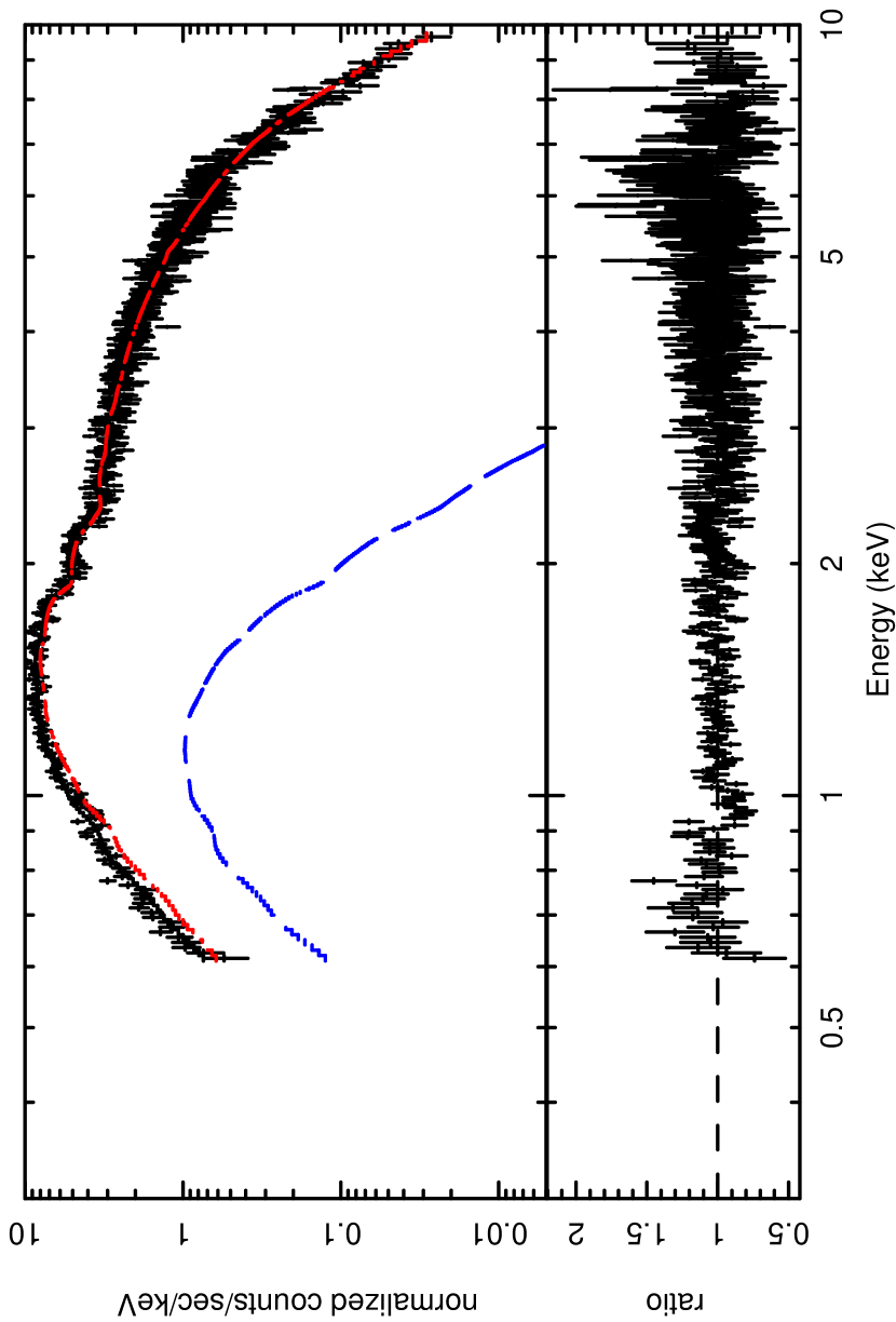
Figure 7.— XRT spectrum of GRO J1655$-$40 for observation 02, in the low/hard state. As in Figure 2, the continuum model is an absorbed accretion disk with a power-law component. The power-law component (red) leaves a soft excess that is consistent with a cool accretion disk (blue).

4. Discussion

Spectral analysis of the X-ray emission from XTE J1817$-$330 during its 2006 outburst shows that the geometrically thin, optically thick accretion disk which dominates the emission in the high-soft state, is also present at or near the innermost stable circular orbit (ISCO) in the low/hard state at very low accretion rates. This is consistent with recent observations of GX 339$-$4, Cygnus X-1, and SWIFT J1753.5$-$0127 (Miller et al., 2006b, a). In the case of XTE J1817$-$330, the flexible scheduling of Swift has made it possible, for the first time, to densely monitor the accretion disk in both X-rays and NUV as it cools and the source transitions from the high/soft state to the low/hard state. Indeed, independently of the exact form of the spectral model chosen, the accretion disk luminosity is shown to be approximately proportional to $T^{4}$, as is predicted for a blackbody of fixed size, and as seen at high accretion rates.

At low accretion rates, the cool accretion disk does not have any significant emission that is visible to RXTE/PCA, which has an effective low energy cutoff of 3 keV. After 2006 June 9, the PCA spectral and timing signatures of XTE J1817$-$330 are consistent with that of the low/hard state (Remillard & McClintock, 2006), when Swift observations still show a prominent accretion disk at $\sim 0.4\,\mathrm{keV}$, as is shown in the middle panel of Figure 2. Although we do not know the distance to XTE J1817$-$330 or the mass of the compact object, we can nevertheless estimate the inner disk radius and accretion rate during the course of the observations, scaled to a nominal distance of $d=10\,\mathrm{kpc}$ and a black hole mass of $M=10\,M_{\sun}$. Then the inner disk radius is $R_{in}=(6\pm 2)\times 10^{1}(d/10\,\mathrm{kpc})/\mathrm{cos}^{-1/2}(\theta)$, where $\theta$ is the disk inclination. This corresponds to $R_{in}=4\pm 1(M/M_{\sun})(d/10\,\mathrm{kpc})/\mathrm{cos}^{-1/2}(\theta)r_{g}$, where $r_{g}=GM/c^{2}$, the Schwarzchild radius, and therefore the inner radius is consistent with the ISCO. The corresponding luminosity during the final observation is $L_{X}=(1.6\pm 0.5)\times 10^{36}(d/10\,\mathrm{kpc})^{2}\,\mathrm{erg}\,\mathrm{s}^{-1}$, or $L_{X}/L_{Edd}=(1.2\pm 0.4)\times 10^{-3}(M/10M_{\sun})(d/10\,\mathrm{kpc})^{2}$, which is a small fraction of the Eddington luminosity.

We find that the NUV (2600 Å) light curve does not track the X-ray light curve. The X-ray flux, which is dominated by the thermal emission, falls much faster than the NUV flux. Furthermore, the NUV flux that is observed is well in excess of an extrapolation of the X-ray disk to lower wavelengths. Thus, the NUV emission is not primarily due to viscous dissipation in the disk. Meanwhile, the $e$-folding time of the NUV light curve is roughly twice the $e$-folding time of the hard X-ray lightcurve. This is consistent with expectations if the optical/NUV emission is dominated by reprocessed hard X-ray emission (King & Ritter, 1998). In addition, there is a strong correlation between the NUV flux and the hard X-ray emission, with a power-law slope of $0.47\pm 0.03$, also consistent with reprocessing. This relationship holds over more than two orders of magnitude in X-ray flux, and is independent of the reddening in the direction of the source.

The above results are consistent with the multi-wavelength observations of the black hole X-ray transient XTE J1859+226 during the 1999-2000 outburst. The optical/UV/X-ray spectral energy distribution (SED) during the early decline was consistent with an irradiation dominated disk extending down to the ISCO (Hynes et al., 2002). Studies of the optical/UV SED of several black hole X-ray transients show that in some cases the UV emission increases towards the far-UV (UV-hard spectra), whereas in others the emission decreases (UV-soft spectra) (Hynes, 2005). In XTE J1859+226 the spectrum evolved from UV-soft to UV-hard, over five UV observations, two of which were simultaneous with X-ray observations. A UV-soft spectrum can be produced in a disk irradiated by a central point source. The UV-hard spectrum can be explained if the disk emission is dominated by viscous dissipation or if the emission is due to X-ray heating from an extended central source such as a jet or a corona (see Hynes 2005 for details). Our results, which do not depend on the reddening in the direction of XTE J1817$-$330, and are based on temporal rather than spectral data, do not suffer from this degeneracy. The multiple epochs of simultaneous NUV and X-ray observations made possible by Swift show in unprecedented detail that the NUV emission is consistent with reprocessed hard X-ray emission in both the high/soft and low/hard states. This would indicate that the irradiating central source of XTE J1817$-$330 is extended, which may well be typical for these black hole X-ray transients.

In this work we have clearly shown that the NUV emission from BHXRBs may be dominated by reprocessed hard X-ray emission. Whereas Russell et al. (2006) came to this conclusion using data from many sources, we see it in detail in an intensive study of a single source. These observations further demonstrate that multi-wavelength emission cannot be assumed to be direct in all cases; the optical/NUV emission and X-ray emission may be from separate components and separate emission regions of the same source.

These results are the strongest evidence yet obtained that accretion disks do not automatically recede after a state transition. Rather, the evolution of the disk temperature appears to be smooth across state transitions, and the inner disk appears to remain at or near the innermost stable circular orbit, at least down to $L_{X}/L_{Edd}\sim 0.001$. We have made a major step forward in being able to demonstrate this result through robust trends, while prior work merely detected disks in the low/hard state. Cool disks with inner radii consistent with the ISCO have been found in every case where good quality soft X-ray spectra have been obtained with a CCD spectrometer, including GX 339$-$4, Cygnus X-1 (Miller et al., 2006b), SWIFT J1753.5$-$0127 (Miller et al., 2006a), XTE J1817$-$330, and GRO J1655$-$40 (this work). However, we must note that geometrically thin accretion disks are likely impossible at the lowest accretion rates observed in black holes, and that an advective flow must take over at some point below $L_{X}/L_{Edd}\sim 0.001$.

References

- Arnaud (1996) Arnaud, K. A. 1996, in ASP Conf. Ser. 101: Astronomical Data Analysis Software and Systems V, ed. G. H. Jacoby & J. Barnes, 17
- Bertin & Arnouts (1996) Bertin, E., & Arnouts, S. 1996, A&AS, 117, 393
- Brocksopp et al. (2006) Brocksopp, C., et al. 2006, MNRAS, 365, 1203
- Burrows et al. (2005) Burrows, D. N., et al. 2005, Space Science Reviews, 120, 165
- Cardelli et al. (1989) Cardelli, J. A., Clayton, G. C., & Mathis, J. S. 1989, ApJ, 345, 245
- Chen et al. (1997) Chen, W., Shrader, C. R., & Livio, M. 1997, ApJ, 491, 312
- D’Avanzo et al. (2006) D’Avanzo, P., et al. 2006, The Astronomer’s Telegram, 724
- Dickey & Lockman (1990) Dickey, J. M., & Lockman, F. J. 1990, ARA&A, 28, 215
- Esin et al. (1997) Esin, A. A., McClintock, J. E., & Narayan, R. 1997, ApJ, 489, 865
- Frank et al. (2002) Frank, J., King, A., & Raine, D. J. 2002, Accretion Power in Astrophysics: Third Edition (Accretion Power in Astrophysics, by Juhan Frank and Andrew King and Derek Raine, pp. 398. ISBN 0521620538. Cambridge, UK: Cambridge University Press, February 2002.)
- Gallo et al. (2003) Gallo, E., Fender, R. P., & Pooley, G. G. 2003, MNRAS, 344, 60
- Gehrels et al. (2004) Gehrels, N., et al. 2004, ApJ, 611, 1005
- Homan et al. (2005) Homan, J., Buxton, M., Markoff, S., Bailyn, C. D., Nespoli, E., & Belloni, T. 2005, ApJ, 624, 295
- Hynes (2005) Hynes, R. I. 2005, ApJ, 623, 1026
- Hynes et al. (2002) Hynes, R. I., Haswell, C. A., Chaty, S., Shrader, C. R., & Cui, W. 2002, MNRAS, 331, 169
- Hynes et al. (1998) Hynes, R. I., et al., 1998, MNRAS, 300, 64
- Hynes et al. (2006) Hynes, R. I., et al. 2006, ApJ, 651, 401
- King & Ritter (1998) King, A. R., & Ritter, H. 1998, MNRAS, 293, L42
- McClintock & Remillard (2006) McClintock, J. E., & Remillard, R. A. 2006, Black hole binaries (Compact stellar X-ray sources), 157–213
- Merloni et al. (2005) Merloni, A., Heinz, S., & Di Matteo, T. 2005, Ap&SS, 300, 45
- Migliari et al. (2005) Migliari, S., Fender, R. P., & van der Klis, M. 2005, MNRAS, 363, 112
- Miller et al. (2004) Miller, J. M., Fabian, A. C., & Miller, M. C. 2004, ApJ, 614, L117
- Miller et al. (2006a) Miller, J. M., Homan, J., & Miniutti, G. 2006a, ApJ, 652, L113
- Miller et al. (2006b) Miller, J. M., Homan, J., Steeghs, D., Rupen, M., Hunstead, R. W., Wijnands, R., Charles, P. A., & Fabian, A. C. 2006b, ApJ, 653, 525
- Miller et al. (2006c) Miller, J. M., Homan, J., Steeghs, D., Torres, M. A. P., & Wijnands, R. 2006c, The Astronomer’s Telegram, 743
- Miller et al. (2006d) Miller, J. M., Homan, J., Steeghs, D., & Wijnands, R. 2006d, The Astronomer’s Telegram, 746
- Mitsuda et al. (1984) Mitsuda, K., et al. 1984, PASJ, 36, 741
- Remillard et al. (2006) Remillard, R., Levine, A. M., Morgan, E. H., Markwardt, C. B., & Swank, J. H. 2006, The Astronomer’s Telegram, 714
- Remillard & McClintock (2006) Remillard, R. A., & McClintock, J. E. 2006, The Astronomer’s Telegram, 836
- Romano et al. (2006) Romano, P., et al. 2006, A&A, 456, 917
- Roming et al. (2005) Roming, P. W. A., et al. 2005, Space Science Reviews, 120, 95
- Rupen et al. (2006) Rupen, M. P., Dhawan, V., & Mioduszewski, A. J. 2006, The Astronomer’s Telegram, 717
- Russell et al. (2006) Russell, D. M., Fender, R. P., Hynes, R. I., Brocksopp, C., Homan, J., Jonker, P. G., & Buxton, M. M. 2006, MNRAS, 371, 1334
- Steeghs et al. (2006) Steeghs, D., Torres, M. A. P., Miller, J., & Jonker, P. G. 2006, The Astronomer’s Telegram, 740
- Titarchuk (1994) Titarchuk, L. 1994, ApJ, 434, 570
- Torres et al. (2006a) Torres, M. A. P., Steeghs, D., Jonker, P. G., Luhman, K., McClintock, J. E., & Garcia, M. R. 2006a, The Astronomer’s Telegram, 733
- Torres et al. (2006b) Torres, M. A. P., Steeghs, D., McClintock, J., Garcia, M., Brandeker, A., Nguyen, D., Jonker, P. G., & Miller, J. M. 2006b, The Astronomer’s Telegram, 749
- van Paradijs & McClintock (1994) van Paradijs, J., & McClintock, J. E. 1994, A&A, 290, 133
- White & Marshall (1984) White, N. E., & Marshall, F. E. 1984, ApJ, 281, 354
- Zimmerman et al. (2005) Zimmerman, E. R., Narayan, R., McClintock, J. E., & Miller, J. M. 2005, ApJ, 618, 832
- Zombeck (1990) Zombeck, M. V. 1990, Handbook of space astronomy and astrophysics (Cambridge: University Press, 1990, 2nd ed.)