Shock oscillation model for QPOs in stellar-mass and supermassive black holes

Abstract

We numerically examine centrifugally supported shock waves in 2D rotating accretion flows around a stellar-mass ($10M_{\odot}$) and a supermassive ($10^{6}M_{\odot}$) black holes over a wide range of input accretion rates of $10^{7}\geq\dot{M}/\dot{M}_{\rm E}\geq 10^{-4}$. The resultant 2D-shocks are unstable with time and the luminosities show quasi-periodic oscillations (QPOs) with modulations of a factor of 2 – 3 and with periods of a tenth seconds to several hours, depending on the black hole masses. The shock oscillation model may explain the intermediate frequency QPOs with 1-10 Hz observed in the stellar-mass black hole candidates and also suggest the existence of QPOs with the period of hours in AGNs. When the accretion rate $\dot{M}$ is low, the luminosity increases in proportion to the accretion rate. However, when $\dot{M}$ exceeds greatly the Eddington critical rate $\dot{M}_{\rm E}$, the luminosity is insensitive to the accretion rate and is kept constantly around $\sim 3L_{\rm E}$. On the other hand, the mass-outflow rate $\dot{M}_{\rm loss}$ increases in proportion to $\dot{M}$ and it amounts to about a few percent of the input mass-flow rate.

1 Introduction

Rotating inviscid and adiabatic accretion flow around a black hole can have two saddle type sonic points. After the flow with adquate injection parameters passes through the outer sonic point, the centrifugal force can virtually stop the rotating supersonic flow, forming a standing shock close to the black hole. Then, the flow passes through the inner sonic point and again falls into the black hole supersonically. In such transonic problems of accretion and wind, Fukue (1987) and Chakrabarti (1989) firstly showed satisfactory analytical or numerical global solutions under a full relativistic treatment and under a pseudo-Newtonian potential, respectively. It has been shown that these generalized accretion flows could be responsible for the hard and soft state transitions or the quasi-periodic oscillations (QPOs) of the hard X-rays from the black hole candidates (Molteni et al., 1996; Ryu et al., 1997; Lanzafame et al., 1998). Further analyses of the transonic problems under modified pseudo-Newtonian potentials showed that the standing shocks are essential ingredients in multi-transonic black hole accretion discs (Das et al., 2001; Das, 2002, 2003) and that the generalized multi-transonic accretion model may show QPO frequencies of Galactic black hole candidates in terms of dynamical flow variables (Das et al., 2003a, b).

Recently, in relative to the shock oscillation models of QPOs, Okuda et al. (2004) and Chakrabarti et al. (2004) showed several numerical simulations of 2D accretion flows around black holes, using the Eulerian method under the treatment of radiation transport and the SPH method in the presence of cooling effects, respectively. From the power spectra of the luminosities, they showed that QPOs are found at a few Hz to hundreds of Hz for stellar-mass black holes with mass of $10M_{\rm\odot}$ and oscillation time-scales of hours to weeks for supermassive black holes with mass of $10^{8}M_{\rm\odot}$. In the present paper, we examine further shock oscillation models over a wide range of accretion rates, focusing on the general properties of the shock waves and the QPO frequencies in the 2D nonadiabatic accretion flows around the black holes.

2 Model Equations

A set of relevant equations consists of six partial differential equations for density, momentum, and thermal and radiation energy. These equations include the heating and cooling of gas and radiation transport. The radiation transport is treated in the gray, flux-limited diffusion approximation (Levermore & Pomraning, 1981). We use spherical polar coordinates ($r$,$\zeta$,$\varphi$), where $r$ is the radial distance, $\zeta$ is the polar angle measured from the equatorial plane of the disc, and $\varphi$ is the azimuthal angle. The gas flow is assumed to be axisymmetric with respect to $Z$-axis ($\partial/\partial\varphi=0$) and the equatorial plane . In this coordinate system, we have the basic equations in the following conservative form (Kley, 1989):

$${\partial\rho\over\partial t}+{\rm div}(\rho\mn@boldsymbol{v})=0,$$ (1)

$${\partial(\rho v)\over\partial t}+{\rm div}(\rho v\mn@boldsymbol{v})=\rho\left[{w^{2}\over r}+{v_{\varphi}^{2}\over r}-{GM_{*}\over(r-r_{\rm g})^{2}}\right]-{\partial p\over\partial r}+f_{r},$$ (2)

$${{\partial(\rho rw)}\over\partial t}+{\rm div}(\rho rw\mn@boldsymbol{v})=-\rho v_{\varphi}^{2}{\rm tan}\zeta-{\partial p\over\partial\zeta}+f_{\zeta},$$ (3)

$${{\partial(\rho r{\rm cos}\zeta v_{\varphi})}\over\partial t}+{\rm div}(\rho r{\rm cos}\zeta v_{\varphi}\mn@boldsymbol{v})=0,$$ (4)

$${{\partial\rho\varepsilon}\over\partial t}+{\rm div}(\rho\varepsilon\mn@boldsymbol{v})=-p\;\rm div\mn@boldsymbol{v}-\Lambda,$$ (5)

and

$${{\partial E_{0}}\over\partial t}+{\rm div}\mn@boldsymbol{F}_{0}+{\rm div}(\mn@boldsymbol{v}E_{0}+\mn@boldsymbol{v}\cdot P_{0})=\Lambda-\rho{(\kappa+\sigma)\over c}\mn@boldsymbol{v}\cdot\mn@boldsymbol{F}_{0},$$ (6)

where $\rho$ is the density, $\mn@boldsymbol{v}=(v,w,v_{\varphi})$ are the three velocity components, $G$ is the gravitational constant, $M_{*}$ is the central mass, $p$ is the gas pressure, $\varepsilon$ is the specific internal energy of the gas, $E_{0}$ is the radiation energy density per unit volume, $P_{0}$ is the radiative stress tensor, and $c$ is the speed of light. The subscript “0” denotes the value in the comoving frame and that the equations are correct to the first order of $\mn@boldsymbol{v}/c$ (Kato et al., 1998). We adopt the pseudo-Newtonian potential (Paczyńsky & Wiita, 1980) in equation (2), where $r_{\rm g}$ is the Schwarzschild radius. The force density $\mn@boldsymbol{f}_{\rm R}=(f_{r},f_{\zeta})$ exerted by the radiation field is given by

$$\mn@boldsymbol{f}_{\rm R}=\rho\frac{\kappa+\sigma}{c}\mn@boldsymbol{F}_{0},$$ (7)

where $\kappa$ and $\sigma$ denote the absorption and scattering coefficients and $\mn@boldsymbol{F}_{0}$ is the radiative flux in the comoving frame. The quantity $\Lambda$ describes the cooling and heating of the gas,

$$\Lambda=\rho c\kappa(S_{*}-E_{0}),$$ (8)

where $S_{*}$ is the source function. For this source function, we assume local thermal equilibrium $S_{*}=aT^{4}$, where $T$ is the gas temperature and $a$ is the radiation constant. For the equation of state, the gas pressure is given by the ideal gas law, $p=R_{\rm G}\rho T/\mu$, where $\mu$ is the mean molecular weight and $R_{\rm G}$ is the gas constant. The temperature $T$ is proportional to the specific internal energy, $\varepsilon$, by the relation $p=(\gamma-1)\rho\varepsilon=R_{\rm G}\rho T/\mu$, where $\gamma$ is the specific heat ratio. To close the system of equations, we use the flux-limited diffusion approximation for the radiative flux:

$$\mn@boldsymbol{F}_{0}=-{\lambda c\over\rho(\kappa+\sigma)}{\rm grad}\;E_{0},$$ (9)

and

$$P_{0}=E_{0}\cdot T_{\rm Edd},$$ (10)

where $\lambda$ and $T_{\rm Edd}$ are the flux-limiter and the Eddington Tensor, respectively, for which we use the approximate formulas given in Kley (1989). The formula fulfill the correct limiting conditions $\lambda\rightarrow 1/3$ in the optically thick diffusion limit, and $\mid\mn@boldsymbol{F}\mid\rightarrow cE_{0}$ as $\lambda\rightarrow 0$ for the optically thin streaming limit.

3 Numerical Methods

The set of partial differential equations (1)–(6) is numerically solved by a finite-difference method under adequate initial and boundary conditions. The numerical schemes used are basically the same as that described previously (Kley, 1989; Okuda et al., 1997). The methods are based on an explicit-implicit finite difference scheme.

3.1 Model Parameters

We consider a stellar-mass black hole with mass $M_{*}=10M_{\odot}$ and a supermassive black hole with $M_{*}=10^{6}M_{\odot}$. To examine the shock model, we determine the injection parameters, such as the specific angular momentum, $\lambda_{\rm out}$, the radial velocity, $v_{\rm out}$, and the sound velocity, $a_{\rm out}$, at an outer boundary radius, $R_{\rm out}$, whose parameters can lead to a shock wave close to the black hole. We search analytically the injection parameters through an examination of the parameter space ($E_{\rm out},\lambda_{\rm out}$), where $E_{\rm out}$ is the total specific energy(Chakrabarti, 1989; Molteni et al., 1994, 1999). The typical model parameters used are listed in Table 1. Here, the velocities and the distances are given in units of $c$ and $r_{\rm g}$, respectively, and $\dot{m}$ is the input accretion rate normalized to the Eddington critical accretion rate $\dot{M}_{\rm E}(=L_{\rm E}/c^{2}$), where $L_{\rm E}$ is the Eddington luminosity given by

$$L_{\rm E}={4\pi GM_{*}c\over{\kappa_{\rm e}}},$$ (11)

and $\kappa_{\rm e}$ is the electron scattering opacity. $L_{\rm E}$ and $\dot{M}_{\rm E}$ are 1.5 $\times 10^{39}$ erg $s^{-1}$ and $1.7\times 10^{18}$ g $s^{-1}$, respectively, for the stellar-mass black hole with $M_{*}=10M_{\odot}$. $\phi$ is the subtended angle of the central black hole to the disc height $h$ at $r=R_{\rm out}$, that is, ${\rm tan}\phi=(h/r)_{\rm out}$. The inner-boundary radius $R_{\rm in}$ of the computational domain is taken to be $2r_{\rm g}$.

Table 1: Model parameters

$M_{*}/M_{\odot}$	$\lambda_{\rm out}$	$v_{\rm out}$	$a_{\rm out}$	$\rho_{\rm out}$($\rm g\;cm^{-3}$)	$\dot{m}$	$\phi$	$R_{\rm out}$
$10$	1.64	0.0751	0.0738	$2.1\times 10^{-12}$ – $7\times 10^{-2}$	$10^{-4}$ – $7\times 10^{6}$	$29^{\circ}$	30
$10^{6}$	1.875	0.0751	0.0654	$2.1\times 10^{-17}$ – $10^{-6}$	$10^{-4}$ – $10^{7}$	$29^{\circ}$	30

3.2 Initial and Boundary Conditions

At the outer-disc boundary we assume a continuous inflow of matter with a constant accretion rate $\dot{M}$ and the injection flow parameters in Table 1. For the accretion rates considered here, we have an optically thick and radiation-pressure dominant accretion flow at the outer boundary $R_{\rm out}=30r_{\rm g}$. Then, the input gas temperature $T_{\rm out}$ is given by

$$(a_{\rm out})^{2}\sim{4\over 3}({P\over\rho})_{\rm out}\sim{4\over 9}({aT^{4}\over\rho})_{\rm out},$$ (12)

where $P$ is the total pressure. Therefore, for a given $a_{\rm out}$, we have a smaller $T_{\rm out}$ for a smaller ambient density $\rho_{\rm out}$. The initial conditions of the flow except the outer-disc boundary are adequately given as a radially hydrostatic equilibrium state with zero azimuthal velocities everywhere. Physical variables at the inner boundary $R_{\rm in}=2r_{\rm g}$, except for the velocities, are given by extrapolation of the variables near the boundary. However, we impose limited conditions that the radial velocities are given by a free-fall velocity and the angular velocities are zero. On the rotational axis and the equatorial plane, the meridional tangential velocity $w$ is zero and all scalar variables must be symmetric relative to these axes. As to the outer boundary region above the outer-disc, we use free-floating conditions and allow for outflow of matter, whereas any inflow is prohibited here. With these initial and boundary conditions, we perform time integration of equations (1)–(6) until a quasi-steady solution is obtained.

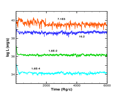
Figure 1: Time evolutions of luminosity $L$ (erg s^-1) for $\dot{m}=1.6\times 10^{-4},1.6\times 10^{-2}$, 16.2, and $7.1\times 10^{5}$ for the stellar-mass black hole.

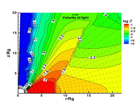
Figure 2: Density contours and velocity vectors at $t=1.2\times 10^{4}\;(r_{\rm g}/c)$ for $\dot{m}=7.1\times 10^{5}$ of the stellar-mass black hole. The standing shock is formed at $r/r_{\rm g}\sim 8$ and $z/r_{\rm g}\leq 3$ near to the equatorial plane but it is bent obliquely toward upstream.

4 Numerical Results

4.1 Stellar-Mass Black Hole

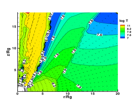
Figure 3: Same as Fig. 2 but temperature contours. The black thick line behind the shocked region shows the funnel wall which is characterized by vanishing effective potential.

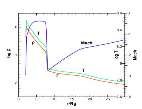
Figure 4: Profiles of density $\rho$ (g cm^-3), temperature $T$ (K), and Mach number of the radial velocity on the equatorial plane at $t=1.2\times 10^{4}\;(r_{\rm g}/c)$ for $\dot{m}=7.1\times 10^{5}$ of the stellar-mass black hole.

The input flow with the injection parameters at the outer-disc radius $R_{\rm out}$ arrives at the innermost radius in a time smaller than $R_{\rm out}/v_{\rm out}(=400r_{\rm g}/c)$ and then the system is settled down toward a quasi-steady state configuration. The luminosity curve is a good measure to check if the quasi-steady state is attained. Fig. 1 shows the time evolutions of luminosity $L$ (erg s^-1) for casese of $\dot{m}=1.6\times 10^{-4},1.6\times 10^{-2}$, 16.2, and $7.1\times 10^{5}$ for the stellar-mass black hole. In each case a quasi-steady state is obtained and the centrifugally supported shock is formed around the black hole. However, the luminosities show QPO phenomena with modulations of a factor of 2 – 3 and the shock positions on the equatorial plane are also found to be variable around several Schwarzschild radii.

The overall features of the flow and the shock are shown in Figs. 2 and 3 which show the contours of density $\rho$ (g cm^-3) and temperature $T$ (K) with velocity vectors at the evolutionary time $t=1.2\times 10^{4}(r_{\rm g}/c)$ for $\dot{m}=7.1\times 10^{5}$, respectively. Here, a spheroidal shock surface is found, where a standing shock exists at $r/r_{\rm g}\sim 8$ and $z/r_{\rm g}\leq 3$ near to the equatorial plane but it is bent obliquely toward upstream. The densities and the temperatures are enhanced by a several factor across the shock surface. Behind the shocked region there exists a funnel wall which is characterized by vanishing effective potential and is roughly denoted by the black thick line in Fig. 3. The extended shocked region between the shock surface and the funnel wall consists of the hot and dense gas with decelerated velocities. The luminosity modulations are caused by oscillations of the hot shocked region. In the cone-like funnel region between the rotational axis and the funnel wall, the temperatures are much higher but the densities are very low, and the gas is optically thin. The accreting matter in the inner shocked region mostly flows into the black hole and partly diverts into the funnel region. The outflow gas generated there is originally subsonic but is accelerated to relativistic velocities due to the radiation pressure force. An upper arrow in Fig. 2 shows the reference velocity vector of light.

Fig. 4 denotes the shock profiles of density $\rho$ (g cm^-3), temperature $T$ (K), and Mach number of the radial velocity on the equatorial plane at the same evolutionary time as Figs. 2 and 3. The radially infalling gas attains to Mach number of $\sim 2.7$ at the shock and is abruptly decelerated across the shock front, and is again supersonically swallowed into the black hole. To understand the transitions of flow variables at the shock, we refer to the pressure balance equation of Rankine–Hugoniot relations:

$$P_{2}+\rho_{2}{v_{2}}^{2}=P_{1}+\rho_{1}{v_{1}}^{2},$$ (13)

where $P$ is the total pressure due to radiation pressure $f_{\rm E}E_{0}$ and gas pressure $R_{\rm g}\rho T/\mu$, $f_{\rm E}$ is the Eddington factor (Kley, 1989), and subscripts “1” and “2” describe quantities before and after the shock.

In the case of $\dot{m}=7.1\times 10^{5}$, the radiation pressure dominates the gas pressure and the gas is optically thick everywhere except the funnel region. The shock features in Figs. 2–4 are very similar to those in the adiabatic flows (Okuda et al., 2004). In Fig. 4, the pre-shock temperature of $\sim 7.5\times 10^{7}$ K jumps to the post-shock temperature of $1.5\times 10^{8}$ K. Here, $f_{\rm E}=1/3,E_{0}=aT^{4},\rho_{1}{v_{1}}^{2}\gg P_{1}$, and $P_{2}\gg\rho_{2}{v_{2}}^{2}$. Then, we have $a{T_{2}}^{4}/3\sim\rho_{1}{v_{1}}^{2}$ from equation (13) and $T_{2}\sim 1.5\times 10^{8}$ K with $\rho_{1}=10^{-1.6}$ g cm^-3 and $v_{1}=0.24$. From the numerical data, $\rho_{2}/\rho_{1}=v_{1}/v_{2}\sim 5$. The gas behaves as an adiabatic flow for a perfect gas with $\gamma=1.5$. The flux limiter $\lambda$ expresses the degree of optical thickness of the gas and $\lambda$ is 1/3 throughout the whole region except the funnel region. On the other hand, for the low accretion rates of $\dot{m}=1.6\times 10^{-2}$ and $1.6\times 10^{-4}$, the gas is optically thin everywhere and the shock features are considerably differ from the adiabatic case, and the shock position near to the equatorial plane moves outward compared with those in the high accretion rates.

Fig. 5 denotes the power energy density spectra of luminosity $L$ (red line) and shock position $R_{\rm s}$ (blue line) on the equatorial plane corresponding to Fig. 1. From the power spectra of $L$, we recognize the QPO-frequencies of a few to 10 Hz and the frequencies increase with increasing $\dot{m}$. The power spectra of $R_{\rm s}$ agree qualitatively with that of $L$.

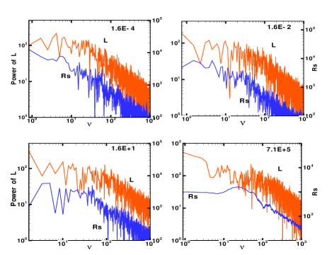
Figure 5: Power energy density spectra of the luminosity $L$ (red line) and the shock position $R_{\rm s}$ (blue line) on the equatorial plane corresponding to Fig. 1.

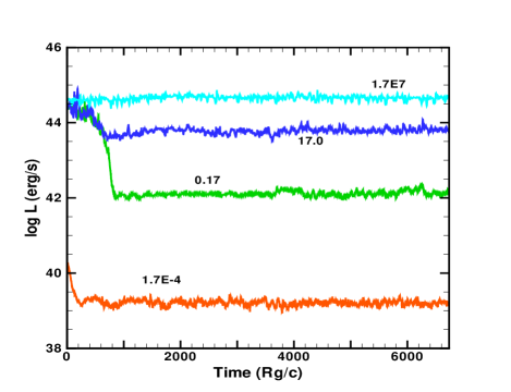
Figure 6: Time evolutions of luminosity $L$ for $\dot{m}=1.7\times 10^{-4}$, 0.17, 17.0, and $1.7\times 10^{7}$ for the supermassive black hole.

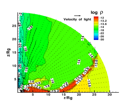
Figure 7: Density contours and velocity vectors at $t=7.4\times 10^{3}(r_{\rm g}/c)$ for $\dot{m}=0.17$ of the supermassive black hole. The oscillating shock near to the equatorial plane is formed at $r/r_{\rm g}\sim$ 12 – 14 and it extends obliquely toward upstream.

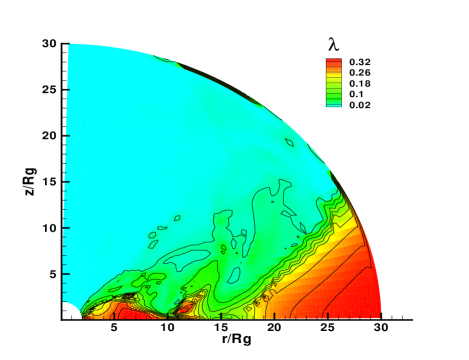
Figure 8: Same as Fig. 7 but the flux-limiter $\lambda$ which shows the degree of optical thickness of the gas.

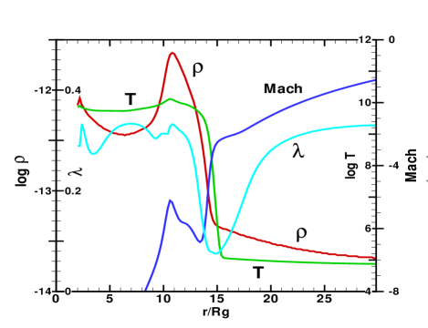
Figure 9: Profiles of density $\rho$ (g cm^-1), temperature $T$ (K), Mach number of the radial velocity, and flux limiter $\lambda$ on the eaqatorial plane at $t=7.4\times 10^{3}\;(r_{\rm g}/c)$ for $\dot{m}=0.17$ of the supermassive black hole.

4.2 Supermassive Black Hole

Fig. 6 shows the luminosity curves for casese of $\dot{m}=1.7\times 10^{-4}$, 0.17, 17.0, and $1.7\times 10^{7}$ for the supermassive black hole. The luminosities show also the quasi-periodic variations with modulations of a factor of 2 – 3. The absolute luminosities are five orders of magnitude larger than those corresponding to the stellar-mass black hole, because of the much larger mass of the supermassive black hole. The general properties of the flows, the shock profiles, and the shock positions for the supermassive black hole are same as those for the stellar-mass black hole. The properties of the flows depend on the input accretion rates. In the high accretion rates, the shock features are same as Figs. 2 – 4 for the stellar-mass black hole and the shock locates at $r/r_{\rm g}\sim$ 7 – 8 on the equatorial plane, as is thoretically predicted in the adiabatic case. However, in the low accretion rates, the accretion flows differ considerably from the cases of high $\dot{m}$.

Figs. 7 and 8 show the contours of density and flux-limiter $\lambda$ with velocity vectors at $t=7.4\times 10^{3}(r_{\rm g}/c)$ for $\dot{m}=0.17$, respectively, where the ambient density $\rho_{\rm out}$ is as low as $\sim 10^{-14}$ g cm^-3. Compared with the flows in Figs. 3 and 4 for the high accretion rate, the accretion flow is geometrically thin in the inner region due to the strong radiative cooling effects. The hot and dense shocked region is confined in a narrow region (red zone in Fig. 7) above the equatorial plane, where the temperatures are as high as $10^{8}$ – $10^{10}$ K. Outside of the shocked region, the densities are very low, so that the gas is optically thin and the temperatures are very high as well. The shock feature near to the equatorial plane is found at $r/r_{\rm g}\sim$ 11 – 14 and it extends obliquely toward upstream. The optically thick input gas becomes optically thin ($\lambda\ll 1/3$) in the pre-shock region and is highly compressed at the shock, and becomes again optically thick ($\lambda\sim 0.3$) in the post-shock region.

The profiles of density $\rho$ (g cm^-3), temperature $T$ (K), Mach number, and flux limiter $\lambda$ on the eqatorial plane are shown in Fig. 9. We find here discontinuous structures of the flow variables like a shock wave in the range of $r/r_{\rm g}$ = 11 – 14 but the flow structures differ considerably from the adiabatic shock solution. Since the upstream temperatures before the discontinuity are as low as $\sim 10^{5}$ K due to the very low input density, the sound velocity is small and Mach number of the infalling gas becomes large. This results in large Mach number of $\sim 6.4$ at the discontinuity. Across the discontinuity, the gas is decelerated down to Mach number $\sim$ 5.2 and is again supersonically falling into the black hole, while the infalling gas never become subsonic after the passage of the outer sonic point and the flow can not have two saddle type sonic points. The discontinuity found in Fig. 9 is eventually regarded as a pseudo-shock front. However, it should be noted that the detailed structures of the horizontal flows at $5\geq z/r_{\rm g}\geq 1$ above the equatorial plane in Fig. 7 show the shock features with the two sonic points and that the shocked regions are joined to the above discontinuity region on the equatorial plane. Then we treat the pseudo-shock like a shock wave to estimate the flow variables before and after the front. Since the gas pressure dominates the radiation pressure in the post-shock region, we have approximately $R_{\rm g}\rho_{2}T_{2}/\mu=\rho_{1}{v_{1}}^{2}$. As the result, the low pre-shock temperature of $\sim 10^{5}$ K jumps to the very high post-shock temperature $T_{2}\sim 10^{10}$ K at the shock. The radiation energy density never change so drastically as the temperature and the density jumps across the shock and is in same order of $\sim a{T_{1}}^{4}$ near to the equatorial plane, so that the radiation pressure dominates the gas pressure in the pre-shock region and the gas pressure is dominant in the post-shock region. The effective thickness of the shock above the equatorial plane becomes broad instead of the discontinuous one in Fig. 4. This agrees with the previous 1D result that the shock thickness broadens with decreasing ambient densities (Okuda et al., 2004).

Fig. 10 denotes the power spectra of luminosity $L$ (red line) and shock position $R_{\rm s}$ (blue line) on the equatorial plane corresponding to Fig. 6. From the power spectra of the luminosities, we find the QPO frequencies $\nu_{\rm qpo}=3\times 10^{-5}$ – $3\times 10^{-4}$ Hz and the period $P_{\rm qpo}=1$ – $10$ hours.

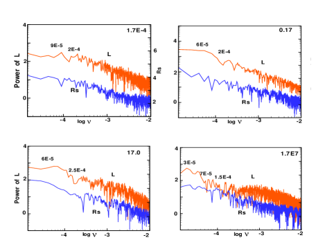
Figure 10: Power energy density spectra of the luminosity $L$ (red line) and the shock position $R_{\rm s}$ (blue line) on the equatorial plane corresponding to Fig. 6

5 Shock Location, Luminosity, and Mass-outflow rate

As to the shock waves examined here, we find general properties of the shock features independent of the black hole masses. This is naturally understood, to some extent, because the injection parameters ($\lambda_{\rm out},v_{\rm out},a_{\rm out}$) have been derived from the dimensionless mass, momentum, and energy conservation equations for the adiabatic gas which are explicitly independent of the black hole masses. There are also common properties of normalized luminosities, shock positions, and mass-outflow rates versus accretion rate $\dot{m}$ between the stellar-mass and the supermassive black holes. Fig. 11 shows the shock position $R_{\rm s}$ versus $\dot{m}$ near to the equatorial plane for the black holes. For $\dot{m}\geq 10^{3}$, $R_{\rm s}/r_{\rm g}\sim$ 7 – 8, while for $\dot{m}\leq$ 1, $R_{\rm s}/r_{\rm g}\sim$ 11 –12. The transition of the former shock position to the latter one occurs in the range of $\dot{m}=1$ – $10^{2}$. The shock positions in the very high accretion rates agree with the theoretical adiabatic solution. In these cases, the gas is optically thick and radiation-pressure dominant, and the radiative cooling term balances the radiative heating one, that is, the radiative energy source $\Lambda\propto(S_{*}-E_{\rm 0})\sim$ 0. Accordingly the flow behaves as the adiabatic flow. However, in the low accretion rates where the gas is optically thin, $S_{*}(=aT^{4})\gg E_{0}$ and the balance of cooling and heating is not established anymore. The source function $\Lambda$ works as the cooling source. At the Rankine–Hugoniot relations of a standing radiative shock in the high accretion rate, the pressure balance is supported by the sum of dominant radiation pressure and ram pressure. When the ambient density is taken to be much lower than that in the high accretion rate, the upstream pressure just before the shock is much smaller because of the lower temperature in the pre-shock region. Therefore, to set up a new pressure balance condition at the shock, the shock must shift outward as far as the same injection parameters are concerened. This is the reason why the decreasing input accretion rate leads to the increasing shock position on the equatorial plane. If the ambient density is taken to be too low, there exists no longer shock wave under the same injection parameters, because the parameters which are originally derived from the adiabatic equations could not match with the optically thin flow.

The QPO-behaviors of the luminosity were attributed to the shock oscillations. We furthermore consider that the shock oscillations are driven by the centrifugal barrier and the radiative cooling in the shocked region (Molteni et al., 1996). When the gas is fully optically thick, the cooling effect is negligible. In the transonic accretion problems around the black hole, it is well known that the transonic flows have generally multi-shock wave solutions, such as the inner and outer shock solutions. The shock waves obtained in this paper correspond to the outer shock wave solution. From the instability analyses of accretion flow with a standing shock wave, it has been found that the outer shock wave both for isothermal and adiabatic flows are dynamically stable (Nakayama, 1994; Nobuta & Hanawa, 1994). On the other hand, when the flow is in an optically thin state, $S_{*}\gg E_{0}$ and the source function $\Lambda\propto\kappa\rho T^{4}$. As the shock is perturbed and propagates outward, it heats the post-shock flow to a higher temperature since the relative velocity between the shock and the incoming flow becomes higher. As a result, the radiative cooling in the post-shock region grows up and the outward motion of the shock stops when the flow is sufficiently cooled down. The shock eventually moves towards the black hole due to the reduced pressure behind the shock. This time, the relative velocity between the shock and the post-shock flow decreases and the post-shock temperature drops. The lower pressure in the post-shock region is unable to balance the preshock ram pressure and the shock collapse continues till the centrifugal barrier is sufficient to hold the flow. The shock then bounces outward and this process is repeated as the shock oscillations. In order to have an oscillatory behavior, the post-shock region must be able to cool in a cooling timescale comparable to the advection timescale at the shock. Thus far, the shock oscillation period is considered as the advection timescale at the shock position $R_{\rm s}$ and the larger $R_{\rm s}$ leads to the larger oscillation timescale and the smaller QPO-frequency. From the power spectra in Figs. 5 and 10, we find that the QPO-frequencies drift to the larger frequencies with increasing $\dot{m}$.

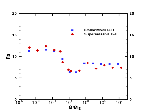
Figure 11: Shock position $R_{\rm s}$ on the equatorial plane versus $\dot{m}$ for cases of the stellar-mass and the supermassive black holes

Fig. 12 shows the normalized luminosity $L/L_{\rm E}$ versus $\dot{m}$ in the wide range of $10^{-4}$ – $10^{7}$. The $L/L_{\rm E}-\dot{m}$ relations are almost identical both for the stellar-mass and the supermassive black holes. When $\dot{M}$ is low, the luminosity increases in proportion to the accretion rate. However, when $\dot{M}$ exceeds greatly the Eddington critical rate $\dot{M}_{\rm E}$, the luminosity is insensitive to $\dot{m}$ and is kept constantly around a maximum luminosity of $\sim 3L_{\rm E}$. We have here approximately

$${\rm log}{L\over L_{\rm E}}=\cases{{\rm log}\;\dot{m}-1.2,\;\;\;\;{\rm for}\;\dot{m}\leq 10^{-2}\cr-0.15\;({\rm log}\;\dot{m})^{2}+0.74\;{\rm log}\;\dot{m}-0.81,\;\;\cr\;\;\;\;\;\;\;\;\;\;\;\;\;\;\;\;\;\;\;\;\;\;\;{\rm for}\;10^{-2}\leq\dot{m}\leq 10^{2},\cr 0.48,\;\;\;\;\;\;\;\;\;\;\;\;\;\;\;{\rm for}\;\dot{m}\gg 10^{2}.\cr}$$ (14)

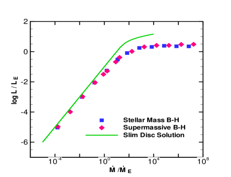
Figure 12: Normalized luminosity $L/L_{\rm E}$ versus $\dot{m}$ for cases of the stellar-mass and the supermassive black holes. The line shows the slim disc solution by Watarai et al. (2000).

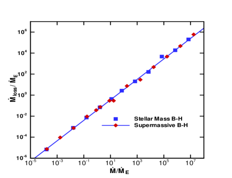
Figure 13: Mass-outflow rate $\dot{M}_{\rm loss}/\dot{M}_{\rm E}$ versus $\dot{m}$ for cases of the stellar-mass and the supermassive black holes.

Watarai et al. (2000) studied the slim-accretion disc model shining at the Eddington luminosity and numerically derived an $L/L_{\rm E}$ - $\dot{m}$ relation. The result is also plotted in Fig. 12. Their $L/L_{\rm E}$ - $\dot{m}$ relation agrees well with ours in the low accretion rates but the luminosities in the high accretion rates are rather larger than ours. The result for the low accretion rates shows $L=0.063\dot{M}c^{2}$, that is, the conversion efficiency $\eta$ of gravitational energy to radiation is $\sim 1/16$. The existence of the maximum luminosity $\sim 3L_{\rm E}$ is interesting from the ultra luminous X-ray sources point of view. The normalized mass-outflow rate $\dot{m}_{\rm loss}(=\dot{M}_{\rm loss}/\dot{M}_{\rm E})$ versus $\dot{m}$ is given in Fig 13. The mass-outflow rate increases in proportion to $\dot{m}$ and we have

$$\dot{M}_{\rm loss}=0.04\;\dot{M}.$$ (15)

The mass-outflow rate $\dot{M}_{\rm loss}$ amounts to about a few percent of the input accretion rate $\dot{M}$.

6 Concluding Remarks

We examined numerically 2D inviscid transonic flows around the stellar-mass and the supermassive black holes, while taking account of the cooling and heating of gas and radiation transport. In these accretion flows, the centrifugally supported shock waves are formed around the black holes. The shock waves are unstable with time and the resultant luminosities show the QPOs with modulations of a factor of 2 – 3. The shock positions are weakly dependent on the accretion rate over a wide range of $\dot{m}$ and are in the range of 7 – 12 $r_{\rm g}$ on the equatorial plane. In the cases of much higher accretion rates ($\dot{m}\gg 1$), the shock position agrees with the theoretical adiabatic solution . On the other hand, the much lower accretion rate leads to the more outward shock position and accordingly the smaller QPO-frequency. As results, we have the QPO frequency $\nu_{\rm qpo}$ of a few to 10 Hz and $3\times 10^{-5}$ – $3\times 10^{-4}$ Hz, that is, the period $P_{\rm qpo}$ of 0.1 – several seconds and 1 – $10$ hours for the stellar-mass and the supermassive black holes, respectively.

Chakrabarti et al. (2004) examined numerically the shock oscillation model around the black holes with masses of $10M_{\rm\odot}$ and $10^{8}M_{\rm\odot}$ and obtained the QPO-frequencies of $\sim$ 8 – 12 Hz and $10^{-7}$ – $10^{-6}$ Hz for the stellar-mass and the supermassive black holes, respectively. We plot the QPO period-mass relation in Fig. 14, together with their results. Here we have approximately

$$P_{\rm qpo}=0.016({M_{*}\over M_{\rm\odot}})\;\;{\rm sec}.$$ (16)

This suggests the QPO-periods expected from the shock oscilation model around black holes in various mass range.

The normalized luminosity and the mass-outflow rate versus $\dot{m}$ have common properties independently on the black hole masses. When $\dot{m}$ is low, the luminosity increases in proportion to the accretion rate. However, when $\dot{M}$ exceeds greatly the Eddington critical rate $\dot{M}_{\rm E}$, the luminosity is insensitive to the accretion rate and is kept constantly around 3 $L_{\rm E}$. On the other hand, the mass-outflow rate $\dot{M}_{\rm loss}$ increases in proportion to $\dot{M}$ and it amounts to a few percent of the input mass-flow rate both for the stellar-mass and the supermassive black holes.

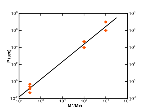
Figure 14: QPO-period $P_{\rm qpo}$ versus black hole mass $M_{*}/M_{\rm\odot}$ due to the shock oscillation model.

The shock oscillation model works only for the accretion flows within a limited parameter space with adequate input parameters for the inviscid flows. Up to now, only the transonic solutions of the accretion flows with total positive energy have been discussed and simulated. However, recent work of the sub-Keplerian flows with negative total energy enlarges the parameter space for which the steady shocks are exhibited in the rotating accretion flows around the black holes (Molteni et al., 2006). Even in the viscous accretion discs, the shock oscillation models are still valid when the viscosity parameter, $\alpha$, is less than a critical value (Molteni et al., 1996; Lanzafame et al., 1998). Of course, if the viscosity is too high, the standing shock disappears.

The centrifugally supported shocks around black holes and the shock oscillation models have been applied to the QPO phenomena in the black hole candidate GRS 1915+105 (Chakrabarti, 1999; Chakrabarti & Manickam, 2000; Rao et al., 2000) in comparison with the observational data. The Galactic X-ray transient source GRS 1915+105 exhibits various types of QPOs: (1) the low-frequency QPO ($\nu_{\rm L}\sim$ 0.001 – 0.01Hz), (2) the intermediate frequency QPO ($\nu_{\rm I}\sim$ 1 – 10Hz), and (3) the high frequency QPO ($\nu_{\rm H}\sim$ 67 Hz) (Morgan, 1997). The QPO-frequencies of a few to 10 Hz due to the shock oscillation model in the stellar-mass black hole may be representative of the intermediate frequency QPO observed in GRS 1915+105.

The shock oscillation model of the supermassive black hole may be applicable to Active Galactic Nuclei, because they are powered by accretion onto a central black hole. Therefore, it may be plausible that QPOs should be observed in AGNs as well. The QPO-frequency due to the shock oscillation model depends on the mass of the supermassive black hole. Recent data of Seyfert galaxies by the EUVE and the Chandra show some periodicities or QPOs in the range of a tenth of hours to a month (Halpern et al., 2003; Moran et al, 2005) and may suggest the relevance to the shock oscillation model. Further observations of the black hole candidates will be needed to confirm the shock oscillation model for QPOs.

References

- Chakrabarti (1989) Chakrabarti, S. K., 1989, ApJ, 347, 365
- Chakrabarti (1999) Chakrabarti, S. K., 1999, A&A, 351, 185
- Chakrabarti et al. (2004) Chakrabarti, S. K., Acharyya., Molteni, D., 2004, A&A, 421, 1
- Chakrabarti & Manickam (2000) Chakrabarti, S. K., Manickam, S. G., 2000, ApJ, 531, L41
- Chakrabarti & Molteni (1993) Chakrabarti, S. K., Molteni, D., 1993, ApJ, 417, 671
- Das (2002) Das, T. K., 2002, ApJ, 577, 880
- Das (2003) Das, T. K., 2003, ApJ, 588, L89
- Das et al. (2001) Das, S., Chattopadhyay, I., Chakrabarti, S. K., 2001, ApJ, 557, 983
- Das et al. (2003a) Das, T. K., Pendharkar, J. K., Mitra, S., 2003a, ApJ, 592, 1078
- Das et al. (2003b) Das, T. K., Rao, A. R., Vadawale, S. V., 2003b, MNRAS, 343, 443
- Fukue (1987) Fukue, J., 1987, PASJ, 39, 309
- Halpern et al. (2003) Halpern, J. M., Leighly, K. M.., Marshall, H. L.., 2003, ApJ, 585, 665
- Kato et al. (1998) Kato, S., Fukue, J., Mineshige, S. ,1998, Black Hole Accretion Disks (Kyoto: Kyoto University Press)
- Kley (1989) Kley, W., 1989, A&A, 208, 98
- Lanzafame et al. (1998) Lanzafame, G., Molteni, D., Chakrabarti, S. K., 1998, MNRAS, 299, 799
- Levermore & Pomraning (1981) Levermore, C. D., Pomraning, G. C., 1981, ApJ, 248, 321
- Molteni et al. (2006) Molteni, D., Gerardi, G., Teresi, V., 2006, MNRAS, 365, 1405
- Molteni et al. (1994) Molteni, D., Lanzafame, G., Chakrabarti, S. K., 1994, ApJ, 425, 161
- Molteni et al. (1996) Molteni, D., Sponholz, H., Chakrabati, S. K., 1996, ApJ, 457, 805
- Molteni et al. (1999) Molteni, D., Toth, G., Kuznetsov, O. A., 1999, ApJ, 516, 411
- Moran et al (2005) Moran, E. C., Eracleous, M., Leighly, K. M., Chartas, G., Filippenko, A. V., Ho, L. C., Blanco, P. R., 2005, AJ, 129, 2108
- Morgan (1997) Morgan, E. H., Remillard, R. A., Greiner, J., 1997, ApJ, 482, 993
- Nakayama (1994) Nakayama K., 1994, MNRAS, 270, 871
- Nobuta & Hanawa (1994) Nobuta K., Hanawa T., 1994, PASJ, 46, 257
- Okuda et al. (1997) Okuda, T., Fujita, M., Sakashita, S., 1997, PASJ, 49, 679
- Okuda et al. (2004) Okuda, T., Teresi, V., Toscano, E., Molteni, D., 2004, PASJ, 56, 547
- Paczyńsky & Wiita (1980) Paczyńsky, B., Wiita, P. J., 1980, A&A, 88, 23
- Rao et al. (2000) Rao, A. R., Naik, S., Vadawale, S. V., Chakrabarti, S. K., 2000, A&A, 360, L25
- Ryu et al. (1997) Ryu, D., Chakrabarti, S. K., Molteni, D., 1997, ApJ, 474, 378
- Watarai et al. (2000) Watarai, K., Fukue, J., Takeuchi, M, Mineshige, S., 2000, PASJ, 52, 133