Spitzer Space Telescope Observations of the Magnetic Cataclysmic Variable AE Aqr

Abstract

The magnetic cataclysmic variable AE Aquarii hosts a rapidly rotating white dwarf which is thought to expel most of the material streaming onto it. Observations of AE Aqr have been obtained in the wavelength range of $5-70\mu$m with the IRS, IRAC, and MIPS instruments on board the Spitzer Space Telescope. The spectral energy distribution reveals a significant excess above the K4V spectrum of the donor star with the flux increasing with wavelength above 12.5 $\mu$m. Superposed on the energy distribution are several hydrogen emission lines, identified as Pf $\alpha$ and Hu $\alpha$, $\beta$, $\gamma$. The infrared spectrum above 12.5 $\mu$m can be interpreted as synchrotron emission from electrons accelerated to a power-law distribution $dN\propto E^{-2.4}dE$ in expanding clouds with an initial evolution timescale in seconds. However, too many components must then be superposed to explain satisfactorily both the mid-infrared continuum and the observed radio variability. Thermal emission from cold circumbinary material can contribute, but it requires a disk temperature profile intermediate between that produced by local viscous dissipation in the disk and that characteristic of a passively irradiated disk. Future high-time resolution observations spanning the optical to radio regime could shed light on the acceleration process and the subsequent particle evolution.

1 Introduction

Multi-wavelength observational investigations of cataclysmic variable (CV) binaries are of continuing interest since they provide important diagnostic information constraining the characteristics of the white dwarf, main sequence like donor, and accretion disk in these systems. Within the last decade, observational studies of CVs at near to mid infrared wavelengths have been carried out in order to determine the spectral type of the mass losing star. Further interest in long wavelength studies of CVs stems from the possibility of detecting cool gas surrounding such systems as its presence can have some affect on the secular evolution of these systems (Spruit & Taam 2001). Circumstantial evidence for the presence of this material had been provided by the existence of faint features characterized by narrow line widths in the optical and far UV spectrum of several objects (e.g., see references in Dubus et al. 2004), although such features are not present in all systems (Belle et al. 2004). Recently, Spitzer Space Telescope observations have revealed the presence of excess infrared emission in magnetic CVs (Howell et al. 2006; Brinkworth et al. 2007) and black hole low-mass X-ray binaries (Muno & Mauerhan 2006).

In view of the accumulating observational evidence for the presence of cool gas surrounding CVs and its possible importance for CV evolution, AE Aquarii was observed with the Spitzer Space Telescope. AE Aqr (catalog ) is a particularly unusual CV as the white dwarf in the system rotates (at 33.08 s) asynchronously with the orbital motion ($P_{orb}=9.88$ hrs). It is highly variable exhibiting flaring behavior in the optical (van Paradijs et al. 1989), radio (Bastian et al. 1988), and ultraviolet (Eracleous & Horne 1996) wavelength regions. More recent observations of AE Aqr in the mid infrared and far infrared wavelengths using ISO (Abada-Simon et al. 2005) have led to the measurement of a crude spectral energy distribution (SED) from $3.6-170\mu$m. Observations in the mid infrared wavelength region were also carried out by Dubus et al. (2004) at Keck Observatory leading to the detection of excess emission in AE Aqr at 12 $\mu$m above that extrapolated from shorter wavelengths and variable on timescales less than an hour.

To significantly improve on the measurement of the SED in the wavelength range from $5-70\mu$m, to identify any possible thermal contribution and to further test the synchrotron emission interpretation for the mid-infrared, based on the multiple injection expanding clouds model (Bastian, Dulk, & Chanmugam 1988) successfully used in the radio regime, we report on the observations of AE Aqr based on measurements obtained with the IRAC, IRS (Infrared Spectrometer), and MIPS (Multiband Imaging Photometer) instruments on the Spitzer Space Telescope. Recently, Harrison et al. (2007) independently reported on the IRS observations. In the next section, we describe the observations and the method of analysis of the Spitzer infrared data. The SED of AE Aqr from combined IRAC, MIPS, IRS and archival data is presented in §3. The implications of these results for CVs are discussed in §4 and summarized in the final section.

2 Observations

2.1 IRAC/MIPS

Observations of AE Aqr were performed with the Infrared Array Camera (IRAC; Fazio et al. 2004) in all four channels (3.6, 4.5, 5.8, and 8.0 $\micron$ ) beginning Julian date 2453501.1. Images were obtained in subarray mode, producing 2 composites of 64 $\times$ 0.1 sec exposures in a 4 point dither pattern for each channel. The final mosaic images were produced for photometric extraction using the Basic Calibrated Data products (pipeline version S12.0.2). Aperture photometry was performed with the IRAF APPHOT package using the standard IRAC 10 pixel aperture radius (12$\arcsec$.2) with a sky annulus extending 10 to 18 pixels (IRAC Data Handbook, Version 3.0, 2006). Since a high SNR ($>$ 23-167) was achieved in all four IRAC channels, the photometric errors in these bands are dominated by an absolute calibration uncertainty of 10%, resulting from the not-yet fully characterized IRAC filter bandpass responses in subarray mode (Quijada et al. 2004, Reach et al. 2005, Hines et al. 2006). The results are listed in Table 1.

AE Aqr was also imaged with the Multiband Imaging Photometer for Spitzer (MIPS; Rieke et al. 2004) at 24 $\micron$ and 70 $\micron$ beginnning Julian date 2453503.8. A single 3 sec exposure was obtained at 24 $\micron$ and a 10 $\times$ 10 sec composite was obtained at 70 $\micron$. Photometry was extracted from the Post Basic Calibrated Data products (pipeline version S12.4.0) using the IRAF APPHOT package. A 13$\arcsec$ aperture radius with a sky annulus extending 20$\arcsec$ to 32$\arcsec$ and aperture correction of 1.167 was used for the MIPS 24 $\micron$ image, whereas, a 35$\arcsec$ aperture radius with sky annulus extending 39$\arcsec$ to 65$\arcsec$ and aperture correction of 1.21 was used for the 70 $\micron$ image. The SNR at 24 $\micron$ and 70 $\micron$ was sufficiently high ($>$100 and 10, respectively) that the photometric uncertainty is dominated by absolute calibration errors of 10% and 20% for MIPS 24 $\micron$ and 70 $\micron$, respectively (MIPS data handbook, Version 3,2, 2006). The total unceratinty for the 70 $\micron$ measurement was obtained by summing in quadrature the 20% absolute calibration error with the inverse of the SNR, resulting in a final error of 22%. The results are also listed in Table 1.

2.2 IRS

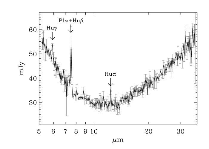
Figure 1: IRS SL-LL spectrum of AE Aqr with line detections indicated. The uncertainties in the fluxes, as derived from the standard deviation from the mean of individual exposures are also shown.

IRS observations of AE Aqr were carried out on 2004 November 13 (Spitzer AOR ID 12699904), as part of the IRS_Disks guaranteed-time observing program. In somewhat different form, the data were analyzed and discussed by Harrison et al. (2007). We used the IRS long-slit, low-spectral-resolution modules ($\lambda/\Delta\lambda~{}=~{}60-100$) to record the 5.3-36 $\mu$m spectrum of AE Aqr. Four 14-second exposures were taken at $\lambda~{}=~{}5.3-14~{}\mu$m, and six 30-second exposures were taken at at $\lambda~{}=~{}14-36~{}\mu$m, divided equally in each case between two sets of observations with the object nodded along the slit by a third of a slit length. We reduced the resulting spectra using the SMART software package (Higdon et al. 2004). Starting with non-flatfielded (”droop”) 2-D spectral data products from the Spitzer Science Center IRS pipeline (version S14), we removed sky emission by subtraction of differently- nodded observations, and extracted signal for each within a narrow window matched to the instrumental point-spread function. The resulting 1-D spectra were multiplied by the ratio of a template spectrum of the A0V star $\alpha$ Lac (Cohen et al. 2003), to identically-prepared IRS observations of this star, to produce calibrated spectra for each exposure. Averaging all of the exposures, we obtain the final spectrum shown in Figure 1.

Like most grating spectrographs, the modules of the IRS respond better to light polarized parallel to the grating rulings than to the orthogonal linear polarization. The ratio of the response in the two linear polarizations is, however, poorly characterized at present. Our observations of AE Aqr were done with the $\lambda~{}=~{}5.3-14~{}\mu$m slit at position angle -22.5°, and the $\lambda~{}=~{}14-36~{}\mu$m slit nearly perpendicular to the other, at -106.1°. These slit orientations are fixed with respect to each other, and cannot be adjusted significantly on the sky for objects as close to the ecliptic plane as AE Aqr. It appears from the continuity of the IRS spectrum at 14 $\mu$m (difference $<4\%$ of the signal) that AE Aqr does not have a large linear polarization in either slit direction at this wavelength. It is possible that the object is more highly polarized at the longest IRS wavelengths than it is at 14 $\mu$m, and because we cannot check the orthogonal polarization at long wavelengths, this possibility adds an unknown additional uncertainty to the flux calibration there; at shorter wavelengths we estimate the photometric uncertainty to be 5% (1$\sigma$).

3 Results

The SED based on the fluxes obtained from the IRS instrument is illustrated in Fig. 1. It can be seen that the flux in the spectrum exhibits a significant excess at longer wavelengths compared to the expected Rayleigh Jeans contribution of the K4V companion star. The flux actually increases at wavelengths longer than 12.5 $\mu$m, as noted by Harrison et al. (2007). In addition to the hydrogen emission lines at 7.5 $\mu$m (Pf $\alpha$ and Hu $\beta$), and 12.4 $\mu$m (Hu $\alpha$) identified by Harrison et al. (2007), we also find evidence for the Hu $\gamma$ transition at 5.9 $\mu$m.

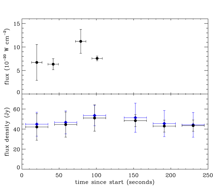
Figure 2: Time dependence of signals during observations. Top panel: flux in the Pf $\alpha$/Hu $\beta$ line blend. Bottom: flux density at 20-28 $\mu$m (circles) and 28-32 $\mu$m (blue diamonds). The time origin of the lower-panel observations is 551 seconds later than that of the upper.

The sensitivity of the observations was sufficient to investigate variability of AE Aqr on the scale of the times of individual exposures. Figure 2 is a plot of the flux in the Pf $\alpha$/Hu $\beta$ blend ($\lambda~{}=~{}7.5~{}\mu$m), and of the continuum flux within bands at $\lambda~{}=~{}20-28~{}\mu$m and $28-32~{}\mu$m, as functions of time. Here, the uncertainties in Fig. 2 were propagated from the IRS noise based uncertainties in each wavelength channel of the individual exposures and (in the case of Pf $\alpha$) the uncertainty in the fit of a Gaussian profile to the line. Although there is a hint of substantial variability in Pf $\alpha$/Hu $\beta$ on minute time scales, the statistical significance is not high (about 2$\sigma$), and thus remains to be confirmed with a longer observation. The long-wavelength continuum bands show no significant variation on minute timescales. Given the uncertainties in each measurement, detecting variability at the 3$\sigma$ level would have required a deviation of 50-100% from the mean flux in one bin. In comparison, Dubus et al. (2004) found 30-50% variability between flux measurements taken about an hour apart at 4.6, 11.3 and 17.6 $\mu$m (with integration times of several minutes).

The overall SED including the fluxes obtained by the IRAC and MIPS instruments is shown in Fig. 3. The fluxes obtained from ISO and IRAS measurements (Abada-Simon et al. 2005), average radio and mm fluxes from Abada-Simon et al. (1993), and Keck measurements in the optical and near infrared are also plotted (Dubus et al. 2004) to provide a spectrum extending over 6 orders of magnitude in frequency. For comparison, the spectrum of a K4V star is fitted to the optical and near infrared data (see Dubus et al. 2004 for details) and is plotted overlaying the SED to illustrate the presence of excess infrared emission for wavelengths longer than 5.8 $\mu$m. The flux measurements for the two long wavebands of the IRAC instrument are not only consistent with those obtained from the IRS instrument, but also with the Keck mid-IR fluxes obtained in 2002. Overall, the average infrared spectrum from 10-100 $\mu$m is well approximated by a $\nu^{-0.7}$ power-law.

4 Discussion

4.1 Non-thermal synchrotron radiation

Non-thermal synchrotron radiation provides a common framework to interpret the SED from radio to mid-infrared frequencies. Although Harrison et al. (2007) considered cyclotron emission from the white dwarf, they concluded that the synchrotron radiation interpretation was more likely, confirming earlier work of Dubus et al. (2004). The inverted radio spectrum is typical of superposed emission from multiple synchrotron self-absorbed components, as seen in X-ray binary and AGN jets. Indeed, Bastian, Dulk, & Chanmugan (1988) modelled the radio emission by multiple clouds of particles undergoing adiabatic expansion. The average spectrum then steepens around $2\times 10^{12}$ Hz to $F_{\nu}\propto\nu^{-0.7}$, as expected for optically thin synchrotron emission from electrons in freshly injected clouds. The required index $p=2.4$, assuming a power-law distribution $dN\propto E^{-p}dE$, is the canonical index derived from shock acceleration theory.

As described in Bastian et al. (1988), the clouds are characterized by their initial radius $R_{0}$, particle density $n_{0}$ and magnetic field $B_{0}$. These values probably change from cloud to cloud but are assumed identical here (representing a time-averaged value). The expansion scales with $\rho\equiv R/R_{0}=(1+t/\beta t_{0})^{\beta}$ with $t_{0}\equiv R_{0}/v_{0}$, and $v_{0}$ the initial expansion velocity. Reproducing the average radio slope $\nu^{0.5}$ with $p=2.4$ requires $\beta\approx 0.53$ (see Eq. 1 in Dubus et al. 2004), faster than expansion in a uniform medium ($\beta$=2/5) but slower than steady expansion ($\beta$=1). Adiabatic cooling arguably dominates since the infrared spectrum up to a few $10^{13}$ Hz appears unaffected by synchrotron or inverse Compton losses, which would steepen the power-law at high frequencies. Requiring that the timescale for adiabatic losses ($t_{0}$) be shorter than the synchrotron timescale of electrons emitting at $10^{13}$ Hz sets an upper limit to $t_{0}$ of $2.4\times 10^{5}B_{0}^{-3/2}\nu_{13}^{-0.5}$ s.

Although the average SED can be reproduced by multiple clouds (see below), reconciling this interpretation with the variability leads to two puzzles. The first is that the variability is not as strong as expected if a single cloud dominated the infrared SED. In this case, the initial optically thin emission would decrease rapidly with time ($F_{\nu}\propto\rho^{-2\beta p}$). Either most of the variability occurs on longer timescales than those sampled in individual observations ($t_{0}\gtrsim 1000$ s) or it occurs very quickly ($t_{0}\lesssim$ 30 s, Fig. 2) and is smoothed out by the continuous ejection of new clouds combined with a coarse time resolution. A long $t_{0}$ is unlikely as radio observations would then show little variability: the peak frequency for a single cloud moves from far-infrared to radio frequencies on a timescale $t\sim 100\,t_{0}(\nu_{12}/\nu_{9})^{0.77}$ so that the variation in radio would be extremely slow. Inversely, observations of radio variability on ks timescales directly set $t_{0}\approx 10$ s. The infrared emission is then the average flux from clouds evolving on a sub-min timescale with an average elapsed time between cloud ejection $t_{\rm flare}\lesssim t_{0}$. This flaring timescale cannot be too long compared to $t_{0}$ (or the peak flux would need to be very high to average out to $\approx 100$ mJy at $2\times 10^{12}$ Hz), nor can it be too short (since then the average SED would require superposing many clouds with small peak flux, implying little variability at any wavelength). The most plausible case appears to be $t_{\rm flare}\sim t_{0}\sim 10$ s. In this case, each 30s bin in Fig. 2 would be an average of three consecutive flares, explaining why the lightcurve shows little variation over 6 min.

Figure 3 shows the average SED expected using $t_{\rm flare}=t_{0}=10$ s, $n_{0}=4.7\times 10^{10}$ cm^-3, $R_{0}=1.3\times 10^{9}$ cm and $B_{0}=1830$ G. To obtain these numbers, which are comparable to those found from the analysis of the radio data by Bastian et al. (1988), an equipartition magnetic field was assumed and the values of the initial peak emission (210 mJy at $3\times 10^{12}$ Hz) were adjusted so as to have the average spectrum peak at about 100 mJy at $2\times 10^{12}$ Hz. The average flux corresponds to the emission from a single cloud integrated over time and multiplied by the flaring rate $t_{\rm flare}^{-1}$. However, if the peak is on average at 40 $\mu$m with a flux of $\approx 50$ mJy, then the multiple clouds interpretation will fail to reproduce the average radio flux.

With the peak position fixed, $B_{0}$, $R_{0}$ and $n_{0}$ are set uniquely by the observations in as much as equipartition is assumed and $t_{\rm flare}=t_{0}$ (regardless of the actual value). A weaker (sub-equipartition) magnetic field would be actually preferable as the synchrotron timescale at 10¹³ Hz for the equipartition field (3 s) is smaller than the adiabatic timescale (10 s). The cloud size compares well with the size of the magnetized blobs through which mass transfer has been proposed to occur in AE Aqr. These blobs approach the white dwarf down to $\approx 10^{10}$ cm at which point the spinning magnetic field of the white dwarf presumably propels them out of the system. Note that $P_{\rm spin}\sim t_{0}$ and that the escape velocity at closest approach is comparable to the expansion velocity $v_{0}=R_{0}/t_{0}\approx 1300$ km s^-1.

Figure 3 also shows the instantaneous emission from a cloud at $t=0$ and $t=t_{0}$ (before a new ejection occurs). Strong variability is expected on a timescale of a few seconds (less than that sampled here by Spitzer) and this can be tested by a high-time resolution mid or far-IR light curve. Emission to near-IR frequencies require electrons of a few 100 MeV. The maximum electron energy is arbitrarily set at 500 MeV in Fig. 3. The high energy electrons contribute a little to the optical $V$-band flux, but this is not sufficient to explain the 0.5 mag flaring that is observed on timescales of minutes (van Paradijs, Kraakman & van Amerongen 1989). Although the flaring at optical (and X-ray) frequencies has also been attributed to propelled gas (Eracleous & Horne 1996), the connection with the non-thermal flaring at low frequencies remains obscure.

The rapid cloud evolution illustrated in Fig. 3 raises the second puzzle. The peak flux from a single cloud varies as $S_{\rm peak}\propto\nu_{\rm peak}^{-1.3}$ so that a cloud initially emitting 100 mJy in infrared can only emit a few 0.1 mJy at most in radio. The radio emission therefore consists of the superposition of hundreds of faint clouds, at odds with the observations of variation of 1-10 mJy in amplitude. A possible solution is that the clouds are re-energized during their expansion (Meintjes & Venter 2003). The variability properties would change, enabling longer variations in infrared to be compatible with the radio flares. Again, a comparison between lightcurves at IR and radio frequencies, notably to characterize lags, would shed light on the conditions during expansion.

4.2 A thermal component?

The circumstantial evidence points towards non-thermal emission. However, in the absence of variability directly linking the infrared emission to the radio, we cannot exclude a contribution from circumbinary material. A multicolor disk blackbody fit to the infrared requires a temperature distribution $T\propto R^{-0.54}$, in between the $-3/7$ slope of a thin disk passively heated by irradiation and the $-3/4$ slope of a thin disk heated by viscous dissipation. We note that a profile of a similar form, $T\propto R^{-1/2}$, has been found from detailed vertical structure models of irradiated accretion disks (D’Alessio et al. 1998) to provide satisfactory fits to the emission properties of young stellar objects (D’Allesio et al. 1999).

The Spitzer data is fitted adequately (Fig. 3) by such a disk extending out to 1.2 AU at a temperature of $55$ K, taking a distance of 102 pc (Friedjung 1997) and an inclination of 55$\arcdeg$. Here, the disk peaks around 40 $\mu$m. This is a better fit than a single temperature (140 K) blackbody (Harrison et al. 2007). Optically thin emission from material at larger distances, and not taken into account here, may contribute to longer wavelengths. The dominant contribution below $\sim 10^{12}$ Hz would still be non-thermal flaring. The contraints on the flare peak frequency and flux are therefore relaxed compared to §4.1, but not enough to account for the amplitude of the radio flares without e.g. re-energizing the clouds.

The expected infrared variability from CB material is slow since the thermal timescale is roughly Keplerian hence $\gtrsim P_{\rm orb}$. Variability on timescales of years might explain the discrepancy between the Spitzer and ISO far-infrared measurements. However, the disk would have to be colder and larger to account for the ISO flux at 90 $\mu$m. The variability seen on a sub-hour timescale by Dubus et al. (2004) argues against thermal infrared emission but has yet to be confirmed by a more extensive set of observations. A disk could be resolved by interferometric observations at mm wavelengths, or possibly in mid-IR where the emission is already a few milli-arcseconds wide. Polarimetric observations may also distinguish between scattered light and synchrotron emission.

4.3 Infrared line emission

The detection of Pf $\alpha$ and Hu $\alpha$, $\beta$ and $\gamma$ in the IRS spectrum is consistent with observations of intense Brackett and Pfund lines in the near-infrared from AE Aqr (Dhillon & Marsh 1995). These lines were attributed to the accretion disk due to their intensity and their widths of $\approx 1500$ km  s^-1 (unfortunately below the IRS spectral resolution). However, high temporal and spectral resolution studies of H$\alpha$ show no disk in AE Aqr and that most of the mass flow from the donor star is probably ejected by the spinning magnetosphere before reaching the white dwarf (Wynn et al. 1997; Welsh et al. 1998). The hydrogen lines are probably produced in the propeller outflow. We note that the combination of intense H line emission and radio emission is reminiscent of outflows in young stellar objects – with the distinction that the radio emission is due to bremsstrahlung in the latter (e.g. Simon et al. 1983).

5 Conclusion

The presence of infrared emission in excess of expectations from the stellar companion in AE Aqr, already present in Keck data up to 17 $\micron$ (Dubus et al. 2004) and in ISO data (Abada-Simon et al. 2005), is confirmed by Spitzer. Synchrotron emission from multiple expanding clouds provides a coherent framework to interpret the SED from radio to infrared wavelengths. Alternatively, interpreting the infrared SED as thermal emission from CB material provides an intriguing parallel with disks surrounding T Tauri stars. This interpretation would still require non-thermal flaring to explain the radio emission and would be ruled out if fast, large amplitude variability is confirmed at infrared wavelengths. On the other hand, synchrotron emission from electrons injected with a canonical $E^{-2.4}$ power-law reproduces well the whole spectrum down to radio frequencies.

However, the multiple cloud picture raises several conundrums. Rapid (seconds) variability is expected in the infrared, but remains undetected, probably for lack of an adequately sampled light curve. In addition, the number of clouds required to reproduce the average radio spectrum is too large to also explain the amplitude of the variations seen at these frequencies (Meintjes & Venter 2003). This requires modification of the basic assumptions adopted by Bastian, Dulk, & Chanmugam (1988). A continuous outflow from the propeller, rather than discrete ejections, may provide a better description of the process operating in AE Aqr. Other questions remain open, such as the nature of the particle acceleration process and the link to the flaring behaviour at optical to X-ray frequencies. Better multiwavelength sampling for short time scale ($<30$ s) spectral evolution studies is needed to obtain further insights into the physics of this unique system.

Table 1: Spitzer Photometry of AE Aquarii

Wavelength	Flux
(${\mu}$m )	(mJy)
3.6	138.9 ${\pm}$ 13.9
4.5	73.2 ${\pm}$ 7.3
5.8	56.1 ${\pm}$ 5.6
8.0	38.2 ${\pm}$ 3.8
24	39.2 ${\pm}$ 3.9
70	52.5 ${\pm}$ 11.6

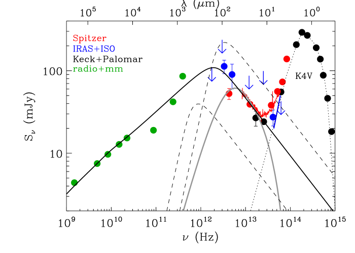
Figure 3: Overall spectral energy distribution of AE Aqr. Spitzer measurements from this work are shown in red (large dots for IRAC and MIPS, red line for IRS spectrum). ISO and IRAS measurements and upper limits are shown in blue (Abada-Simon et al. 2005). The blue line represents the ISOCAM spectrum. The black dots show the lower values of the UBVRIJHK measurements obtained at Palomar and the average M, 11.6 $\mu$m and 17.6 $\mu$m measurements obtained with Keck in 2002 (Dubus et al. 2004). The black dotted line is a K4V star fit to the optical and near-IR data illustrated for comparison. The green dots are average radio and mm fluxes taken from Abada-Simon et al. (1993, 2005). The solid black line is the average emission from clouds ejected on a timescale $t_{\rm flare}$=10 s and cooling adiabatically on the same timescale (§4.1). The dashed lines show the instantaneous spectrum emitted by a single cloud at $t=0$ and at $t=10$ s, just before a new cloud flares. Alternatively, the solid grey line is the emission from an optically thick circumbinary disk with $T\propto R^{-0.54}$ and a temperature of 55 K at its maximum radius of 1.2 AU (§4.2).

References

- Abada-Simon et al. (1993) Abada-Simon, M. Lecacheux, A., Bastian, T. S., Bookbinder, J. A., Dulk, G. A. 1993, ApJ, 406, 692
- Abada-Simon et al. (2005) Abada-Simon, M. et al. 2005, A&A, 433, 1063
- Bastian, Dulk & Chanmugan (1988) Bastian, T. S., Dulk, G. A., & Chanmugam, G. 1988, ApJ, 324, 431
- Belle et al. (2004) Belle, K. E., Sanghi, N., Howell, S. B., Holberg, J. B., & Williams, P. T. 2004, AJ, 128, 448
- Brinkworth et al. (2007) Brinkworth, C. S., et al. 2007, ApJ, in press, ArXiv Astrophysics e-prints, arXiv:astro-ph/0701307
- Cohen et al. (2003) Cohen, M., Megeath, S. T., Hammersley, P. L., Fabiola, M., & Stauffer, J. 2003, AJ, 125, 2645
- (7) D’Alessio, P., Calvet, N., Hartmann, L, Lizano, S., Canto, J. 1999, ApJ, 527, 893
- (8) D’Alessio, P., Canto, J., Calvet, N., & Lizano, S. 1998, ApJ, 500, 441
- Dhillon & Marsh (1995) Dhillon, V. S., & Marsh, T. R. 1995, MNRAS, 275, 89
- Dubus et al. (2004) Dubus, G., Campbell, R., Kern, B., Taam, R. E., & Spruit, H. C. 2004, MNRAS, 349, 869
- Eracleous & Horne (1996) Eracleous, M., & Horne, K. 1996, ApJ, 471, 427
- (12) Fazio, G. et al., 2004, ApJS, 154, 10 (IRAC instrument reference)
- (13) Friedjung M., 1997, New Astron. 2, 319
- Harrison et al. (2007) Harrison, T. E., Campbell, R. K., Howell, S. B., Cordova, F. A., & Schwope, A. D. 2007, ApJ, 656, 444
- Higdon et al. (2004) Higdon, S. J. U., Devost, D., Higdon, J. L., Brandl, B. R., Houck, J. R., Hall, P., Barry, D., Chamandaris, V., Smith, J. D. T., Sloan, G. C., & Green, J. 2004, BAAS, 116, 975
- (16) Hines, D. et al. 2006, ApJ, 638, 1070
- Howell et al. (2006) Howell, S. B., et al. 2006, ApJ, 646, L65
- Meintjes & Venter (2003) Meintjes, P. J., & Venter, L. A. 2003, MNRAS, 341, 891
- Muno & Mauerhan (2006) Muno, M. P., & Mauerhan, J. 2006, ApJ, 648, L135
- (20) Quijada, M. A., Marx, C. T., Arendt, R. G., & Moseley, S. H. 2004, Proc. SPIE, 5487, 244
- (21) Reach, W. T. et al. 2005a, PASP, 117, 978
- (22) Rieke, G. et al. 2004, ApJS, 154, 25 (MIPS instrument reference)
- Simon et al. (1983) Simon, M., Felli, M., Massi, M., Cassar, L., & Fischer, J. 1983, ApJ, 266, 623
- Spruit & Taam (2001) Spruit, H. C., & Taam, R. E. 2001,ApJ, 561, 329
- van Paradijs, Kraakman & van Amerongen (1989) Van Paradijs, J., Kraakman, H., & van Amerongen, S. 1989, A&AS, 79, 205
- Welsh et al. (1998) Welsh, W. F., Horne, K., & Gomer, R. 1998, MNRAS, 298, 285
- Wynn et al. (1997) Wynn, G. A., King, A. R., & Horne, K. 1997, MNRAS, 286, 436