Galaxy Evolution from Halo Occupation Distribution Modeling of DEEP2 and SDSS Galaxy Clustering

Abstract

We model the luminosity-dependent projected two-point correlation function of DEEP2 and SDSS galaxies within the Halo Occupation Distribution (HOD) framework. From this we infer the relationship between galaxy luminosity and host dark matter halo mass at $z\sim 1$ and at $z\sim 0$. At both epochs, there is a tight correlation between central galaxy luminosity and halo mass, with the slope and scatter decreasing for larger halo masses, and the fraction of satellite galaxies decreasing at higher luminosity. Central $L_{*}$ galaxies reside in halos a few times more massive at $z\sim 1$ than at $z\sim 0$. The satellite fraction of galaxies more luminous than $L_{*}$ is $\sim$10% at $z\sim 1$, compared to $\sim$20% at $z\sim 0$. We find little evolution in the relation between the characteristic minimum mass of a halo hosting a central galaxy above a luminosity threshold and the mass scale of a halo that on average hosts one satellite galaxy above the same luminosity threshold, with the latter being 15–20 times the former. Combining these HOD results with theoretical predictions of the typical growth of halos, we establish an evolutionary connection between the galaxy populations at the two redshifts by linking $z\sim 0$ central galaxies to $z\sim 1$ central galaxies that reside in their progenitor halos, which enables us to study the evolution of galaxies as a function of halo mass. We find that the stellar mass growth of galaxies depends on halo mass. On average, the majority of the stellar mass in central galaxies residing in $z\sim 0$ low-mass halos ($\sim 5\times 10^{11}h^{-1}M_{\odot}$) is the result of star formation between $z\sim 1$ and $z\sim 0$, while only a small fraction of the stellar mass in central galaxies of high mass halos ($\sim 10^{13}h^{-1}M_{\odot}$) is the result of star formation over this period. In addition, the mass scale of halos where the star formation efficiency reaches a maximum is found to shift toward lower mass with time. With appropriately defined galaxy samples at different redshifts, future work can combine HOD modeling of the clustering with the assembly history and dynamical evolution of dark matter halos. This can lead to an understanding of the stellar mass growth due to both mergers and star formation as a function of host halo mass and provide powerful tests of galaxy formation theories. In the appendix, we provide a brief discussion of systematic biases related to the assumption of “one galaxy per halo” in estimating the mass scale and number density of host halos from the observed clustering strength of galaxies.

1. Introduction

The spatial clustering of galaxies encodes useful information about their formation and evolution, which remain outstanding problems in modern cosmology and astrophysics. Large redshift surveys at different epochs have enabled detailed studies of galaxy clustering and its evolution. In particular, the dependence of clustering on galaxy properties such as luminosity and color provides fundamental constraints on galaxy formation theories. In this paper, we model the luminosity-dependence of the galaxy two-point correlation functions at $z\sim 1$ and $z\sim 0$ measured for galaxies in the DEEP2 Galaxy Redshift Survey (Coil et al., 2006a) and the Sloan Digital Sky Survey (SDSS; (Zehavi et al., 2005) to investigate the evolution of galaxies over the last $\sim$7 billion years.

To make full use of the galaxy clustering measurements to test galaxy formation theories, one needs to extract and characterize the information available in the clustering data in a convenient and informative form. In the cold dark matter (CDM) hierarchical structure formation paradigm, the evolution of galaxies is coupled to that of the dark matter halos, defined as roughly spherical, virialized regions with over-density about 200 times that of the mean background density. The formation and evolution of dark matter halos are dominated by gravity and, with the help of improving computational power and $N$-body simulations, can be calculated accurately for any specified cosmological model. Galaxy clustering data are particularly illuminating if one can relate galaxies to dark matter halos in a way that results in informative tests of galaxy formation theory. This can be achieved within the framework of the halo occupation distribution (HOD), which describes the statistical relation between galaxies and dark matter halos (see e.g., Jing, Mo, & Börner 1998; Ma & Fry 2000; Peacock & Smith 2000; Seljak 2000; Scoccimarro et al. 2001; Berlind & Weinberg 2002; Cooray & Sheth 2002). The HOD characterizes this relation in terms of the probability distribution $P(N|M)$ that a halo of virial mass $M$ contains $N$ galaxies of a given type and the relative spatial and velocity distribution of galaxies and dark matter within halos.

Contemporary large galaxy surveys, such as the SDSS (York et al., 2000) and the Two-Degree Field Galaxy Redshift Survey (2dFGRS; Colless et al. 2001), enable detailed studies of the $z\sim 0$ galaxy population. HOD modeling, or the closely related “conditional luminosity function” (CLF) method (Yang, Mo, & van den Bosch, 2003), has been applied to interpret clustering data from these local surveys (e.g., Jing & Börner 1998; Jing, Börner, & Suto 2002; van den Bosch et al. 2003; Magliocchetti & Porciani 2003; Zehavi et al. 2005; Yang et al. 2005). Recently, much effort has also been placed on studying the clustering of high redshift galaxies, from $z\lesssim 1$, such as the DEEP2 survey (Davis et al., 2003), the COMBO-17 survey (Classifying Objects with Medium Band Observations in 17 filters; Wolf et al. 2004), the NDWFS (NOAO Deep Wide-Field Survey; Jannuzi & Dey 1999), and the VVDS (VIMOS-VLT Deep Survey; Le Fevre et al. 2005), up to $z\sim 3$–$5$ in many surveys (e.g., Adelberger et al. 2005a, b; Lee et al. 2006; Ouchi et al. 2004, 2005; Allen et al. 2005; Hildebrandt et al. 2005; Daddi et al. 2003). HOD/CLF modeling has also been used to explain the clustering properties of these high redshift galaxies (e.g., Bullock, Wechsler, & Somerville 2002; Moustakas & Somerville 2002; Yan, Madgwick, & White 2003; Zheng 2004; Lee et al. 2006; Hamana et al. 2006; Cooray 2005, 2006; Cooray & Ouchi 2006; Conroy et al. 2006; White et al. 2007; Blake et al. 2007). Galaxy clustering data at different redshifts provide a goldmine of information from which to deepen our understanding of galaxy evolution. As an example, White et al. (2007) find evidence for merging or disruption of red galaxies in NDWFS from modeling the evolution of their clustering. Recent studies of galaxy luminosity functions and two-point correlation functions at different redshifts with the CLF approach also reveal some interesting evolutionary trends, such as a brightening of the luminosity of central galaxies at a fixed halo mass toward higher redshifts (e.g., Cooray 2005).

As galaxies evolve, they grow in both stellar and dark matter mass. Their stellar component continuously changes as the original stars age and new stars form. Galaxies can also change their stellar contents and increase their mass as a result of mergers with other galaxies. Different feedback or pre-heating mechanisms, such as those caused by star formation, active galactic nuclei, or the photo-ionizing ultra-violet background, can also impact at different stages of a galaxy’s life. Various evolutionary processes can change galaxy properties such as luminosity, color, mass and morphology. To observationally establish a connection between galaxy populations at different redshifts is therefore not trivial. Much of the work to identify progenitors or descendants of certain galaxy types from galaxy clustering has been based on rather simple models with limited constraining power, such as the object-conserving or the merging model (Matarrese et al., 1997; Moscardini et al., 1998). By contrast, the HOD framework converts the observed galaxy clustering data to a relation between galaxies and their host dark matter halos, placing galaxies in a cosmological context. Using HOD constraints at different redshifts derived from clustering data thus provides a physically motivated way to study galaxy evolution.

The evolution of the HOD reflects how the relation between galaxies and halos changes with time, which can be used to test galaxy formation models in a more transparent way. The evolution of dark matter halos can be solved with analytic approaches (e.g., Taylor & Babul 2001, 2004; Benson et al. 2002; Oguri & Lee 2004; van den Bosch et al. 2005; Zentner et al. 2005) and cosmological simulations (e.g., Springel et al. 2005). Thus, the HOD evolution may potentially provide valuable constraints on the evolution of baryons in galaxies (e.g., accretion and consumption of gas, formation of stars) and put powerful tests on galaxy formation theories. Many recent studies of galaxy evolution have measured specific galaxy properties (e.g., the star formation rate or the star formation history) as a function of the mass of the galaxy, where either the stellar mass or an estimate of the dynamical mass is used (e.g., Heavens et al. 2004; Jimenez et al. 2005; Juneau et al. 2005; Bundy et al. 2006; Cimatti et al. 2006; Erb et al. 2006a, b; Jimenez et al. 2006; Noeske et al. 2007a, b; Zheng et al. 2007). The unique aspect of the approaches presented and envisioned in this paper that make use of HOD modeling of galaxy clustering at different redshifts is that we are able to study the evolution of galaxy properties as a function of the host dark matter halo mass, which is a fundamental parameter in galaxy formation and evolution.

In this paper we perform HOD modeling of the luminosity dependence of the galaxy two-point correlation function for samples at two epochs, the $z\sim 1$ DEEP2 galaxies and the $z\sim 0$ SDSS galaxies, to study the evolution of the HOD and its implication for galaxy formation models. The structure of the paper is as follows. In § 2 we briefly describe the DEEP2 and SDSS galaxy samples used here. We define our cosmological model and introduce the HOD parameterization in § 3. The modeling results are presented in § 4. In § 5 we make a detailed comparison between the HODs at the two epochs. In § 6 we attempt to establish an evolutionary link between the two galaxy populations through the growth of dark matter halos. This allows us to infer the evolution of galaxies as a function of the host halo mass during the last $\sim$7 billion years. We also discuss the star formation efficiency at the two epochs. Finally, in § 7 we summarize our results and discuss how to extend the study in this paper to a powerful, comprehensive program to constrain galaxy formation and evolution theories. For a simple estimate, instead of using a full HOD modeling, some applications of galaxy clustering assume one galaxy per halo. In the Appendix we use an HOD model to investigate the potential systematic errors introduced by this assumption.

2. Galaxy Samples

2.1. DEEP2 Samples

We use the projected two-point correlation functions measured by Coil et al. (2006a) for luminosity threshold galaxy samples from the DEEP2 Galaxy Redshift Survey to constrain the HOD at $z\sim 1$. The DEEP2 survey uses DEIMOS (Faber et al., 2003) on the 10-m Keck II telescope to survey optical galaxies at $z\sim 1$ in a comoving volume of approximately 5$\times$10⁶ $h^{-3}$Mpc³. DEEP2 has measured redshifts for $>30,000$ galaxies in the redshift range $0.7<z<1.45$ to a limiting magnitude of $R_{\rm AB}=24.1$ over 3 deg² of the sky. Technical details of the DEEP2 survey can be found in Davis et al. (2003) and Davis, Gerke, & Newman (2004).

Here we use the four nearly volume-limited samples of Coil et al. (2006a), defined by thresholds in rest-frame Johnson $B$ absolute magnitude ($M_{B}$). $K$-corrections are calculated as described in Willmer et al. (2006), and no corrections are made for luminosity evolution. Each sample has a minimum redshift of $z=0.75$ and a maximum redshift of $z=1.0-1.2$, depending on luminosity, and includes 5000–11,000 galaxies. The three brightest samples ($M_{B}<-20.5$, $M_{B}<-20.0$, and $M_{B}<-19.5$) are volume-limited for blue galaxies, while the faintest sample ($M_{B}<-19.0$) is missing some fainter blue galaxies at $0.95<z<1.0$. The samples are not entirely volume-limited for red galaxies, due to the $R_{\rm AB}$ selection of the DEEP2 survey (for definitions of blue and red galaxies and a discussion of this selection effect see Willmer et al. 2006). By assuming little evolution in the red galaxy fraction at $z\sim 1$ and using a volume-limited (but smaller) control sample at a slightly lower redshift, we estimate that, for each sample, about 10% of the full population is missed because of the red galaxies being not volume-limited. We address the impact of this sample selection on the galaxy evolution we attempt to establish in § 6.

2.2. SDSS Samples

We compare the DEEP2 clustering and modeling results to those obtained from the SDSS at lower redshifts. The SDSS (York et al. 2000; Stoughton et al. 2002) is an ongoing project that aims to map nearly one quarter of the sky in the northern Galactic cap, as well as a small portion of the southern Galactic cap, using a dedicated 2.5m telescope (Gunn et al., 2006). A drift-scanning mosaic CCD camera (Gunn et al., 1998) is used to image the sky in five photometric bandpasses to a limiting magnitude of $r\sim 22.5$. Objects are selected for spectroscopic follow-up using specific algorithms for the main galaxy sample (Strauss et al., 2002), luminous red galaxy sample (Eisenstein et al., 2001), and quasars (Richards et al., 2002). To a good approximation, the main galaxy sample consists of all galaxies with Petrosian magnitude $r<17.77$, with a median redshift of $\sim 0.1$. The construction of the large-scale structure samples is described in detail in Blanton et al. (2005). The radial selection function is derived from the sample selection criteria using the $K$-corrections of Blanton et al. (2003a) and an improved version of the evolving luminosity function model of Blanton et al. (2003b). The angular completeness is characterized carefully for each sector (a unique region of overlapping spectroscopic plates) on the sky.

We use here the clustering results presented in Zehavi et al. (2005) for an SDSS sample containing some $200,000$ galaxies extending over $\sim 2500$ deg² on the sky. More specifically, we use the projected two-point correlation function measurements for volume-limited samples defined by thresholds in $r$-band absolute magnitude ($M_{r}$). These luminosity threshold samples span a redshift range of $0.02<z<0.22$. Zehavi et al. (2005) have also performed detailed HOD modeling of these clustering measurements. We build on these results, although in order to facilitate a more direct comparison to the DEEP2 modeling presented here, we repeat the SDSS HOD modeling with a slightly different and more flexible suite of models used in this work.

The SDSS and the DEEP2 surveys have different sample selections, with SDSS galaxies selected in rest-frame $r$-band and DEEP2 galaxies in rest-frame $B$-band. The differences in the selection complicate the comparison of the HOD modeling results, a point we address throughout the paper.

3. Cosmology and HOD Models

3.1. Cosmology and Halo Properties

We adopt a spatially-flat CDM cosmological model with Gaussian initial density fluctuations that is consistent with the determination from the cosmic microwave background, Type Ia supernovae, and galaxy clustering (e.g., Spergel et al., 2003, 2007; Riess et al., 2004; Tegmark et al., 2004; Abazajian et al., 2005). Density parameters are assumed to be ($\Omega_{m}$, $\Omega_{\Lambda}$, $\Omega_{b}$)=(0.3, 0.7, 0.047), where $\Omega_{m}$, $\Omega_{\Lambda}$, and $\Omega_{b}$ are density parameters of the matter (CDM+baryons), dark energy, and baryons, respectively. The mass fluctuation power spectrum is the primordial power spectrum, with the spectral index assumed to be $n_{s}$=1, modified by the transfer function, which is computed using the formula given by Eisenstein & Hu (1998) with the effect of baryons taken into account. It is normalized such that the rms fluctuation of the linear density in spheres of radius 8$h^{-1}{\rm Mpc}$ at $z$=0 is $\sigma_{8}$=0.9. The Hubble constant is $H_{0}\equiv 100h=70\,{\rm km\,s}^{-1}{\rm Mpc}^{-1}$.

We define a dark matter halo as an object with mean density of 200 times that of the background universe. With the assumed cosmological model, properties of dark matter halos are calculated based on numerically tested fitting formulas. The halo mass function is computed according to the formula given by Jenkins et al. (2001). For the large-scale halo bias factor, we adopt the formula in Tinker et al. (2005), which is a modification of that given by Sheth et al. (2001) and is accurate for a large range of cosmological parameters. The density distribution of a dark matter halo of mass $M$ is assumed to follow the Navarro-Frenk-White (NFW) profile (Navarro, Frenk, & White, 1995, 1996, 1997) characterized by the concentration parameter $c(M)$. For $c(M)$, we use the relation given by Bullock et al. (2001), modified to be consistent with our halo definition,

$$c(M)=\frac{c_{0}}{1+z}(M/M_{*})^{\beta},$$ (1)

where $c_{0}=11$, $\beta=-0.13$, and $M_{*}$ is the nonlinear mass at $z=0$ ($M_{*}=7.77\times 10^{12}h^{-1}M_{\odot}$ for the adopted cosmology).

3.2. HOD Parameterization

It has proven to be useful to parameterize the HOD by separating contributions from central and satellite galaxies, through studies of subhalo HODs in high-resolution, dissipationless $N$–body simulations (Kravtsov et al., 2004) and galaxy HODs in semi-analytic galaxy formation model (SA) and in smoothed particle hydrodynamics (SPH) simulations (Zheng et al., 2005). For galaxy samples defined by lower luminosity thresholds, a simple parameterization of the mean occupation function has three parameters (e.g., Kravtsov et al., 2004; Zheng et al., 2005; Zehavi et al., 2005) — the mean occupation function $\langle N_{\rm cen}(M)\rangle$ of central galaxies can be represented by a step-like function with a characteristic minimum halo mass $M_{\rm min}$, and the mean occupation function $\langle N_{\rm sat}(M)\rangle$ of satellite galaxies is approximated by a power law with the amplitude and slope as two free parameters. This simple three-parameter model can capture the basic features in the mean occupation function predicted by galaxy formation models.

However, there are some advantages in choosing a parametrization more flexible than the simple one. For example, at lower halo mass, the mean occupation function of satellites predicted by galaxy formation models drops faster than the extrapolation of the high mass power law (Kravtsov et al., 2004; Zheng et al., 2005). Since, in the low-mass range, satellites have a substantial contribution to the galaxy two-point correlation function, with the simple three-parameter model, the best-fit power law slope in the satellite mean occupation function tends to reflect the effective slope in the low-mass range (e.g., Zehavi et al., 2005). That is, the overall slope is adjusted to fit the amplitude of $\langle N_{\rm sat}\rangle$ in the low-mass range, and it may become a poor description for the slope at high halo mass.

In this paper we adopt a slightly more flexible parameterization with five parameters, motivated by the results presented in Zheng et al. (2005). The mean occupation function of the central galaxies is a step-like function with a soft cutoff profile to account for the scatter between galaxy luminosity and host halo mass. That of the satellite galaxies is a power law modified by a low-mass cutoff profile in better agreement with predictions of galaxy formation models. This more flexible parameterization includes two parameters for the mean occupation function of central galaxies and three for that of the satellite galaxies, which are described in detail below.

The mean occupation function of central galaxies is a step-like function parameterized by

$$\langle N_{\rm cen}(M)\rangle=\frac{1}{2}\left[1+{\rm erf}\left(\frac{\log M-\log M_{\rm min}}{\sigma_{\log M}}\right)\right],$$ (2)

where ${\rm erf}$ is the error function

$${\rm erf}(x)=\frac{2}{\sqrt{\pi}}\int_{0}^{\rm{x}}e^{-t^{2}}dt.$$ (3)

There are two free parameters: $M_{\rm min}$, the characteristic minimum mass of halos that can host central galaxies above the luminosity threshold, and $\sigma_{\log M}$, the width of the cutoff profile. Note that $M_{\rm min}$ here can be interpreted as the mass of such halos for which half of them host galaxies above the given luminosity threshold, i.e., $\langle N_{\rm cen}(M_{\rm min})\rangle=0.5$. It is not identical to those used in three-parameter models (e.g., Zehavi et al. 2005): $\langle N_{\rm cen}(M_{\rm min})\rangle=1/e$ for an exponential cutoff profile and $\langle N_{\rm cen}\rangle$ changes from 0 to 1 at $M_{\rm min}$ for a sharp cutoff profile. Nevertheless, in all cases, $M_{\rm min}$ characterizes the minimum mass scales of the host halos. In the three-parameter model, $\langle N_{\rm cen}(M)\rangle$, which uses one parameter $M_{\rm min}$, can also have a soft cutoff profile, e.g., an exponential profile as in Zehavi et al. (2005). However, the two parameters $M_{\rm min}$ and $\sigma_{\log M}$ of the cutoff profile in equation (2) have a more physical meaning. To see this, we briefly review the derivation of the form of $\langle N_{\rm cen}(M)\rangle$. The motivation for such a form is the relation between the central galaxy luminosity and the host halo mass predicted by galaxy formation models. Based on predictions of SA and SPH galaxy formation models, Zheng et al. (2005) show that the distribution of the central galaxy luminosity $L_{c}$ at fixed halo mass $M$ can be described by a log-normal distribution, and here we write it as

$$P(\log L_{c}|M)=\frac{1}{\sqrt{2\pi}\sigma_{\log L}}\exp\left[-\frac{(\log L_{c}-\log\langle L_{c}(M)\rangle)^{2}}{2\sigma_{\log L}^{2}}\right].$$ (4)

In halos of mass $M$, the mean occupation function of the central galaxies above a luminosity threshold $L_{\rm min}$ is an integration of equation (4) over $\log L_{c}$, and the result turns out to have the same form as equation (2) but with the argument of the ${\rm erf}$ function being $[\log L_{\rm min}-\log\langle L_{c}(M)\rangle]/(\sqrt{2}\sigma_{\log L})$. If the mass range of the cutoff profile is not large so that we can approximate the mean luminosity $\langle L_{c}(M)\rangle$ of central galaxies in halos of mass $M$ as $\langle L_{c}(M)\rangle\propto M^{p}$, it is straightforward to see the meaning of the parameters in equation (2) — $M_{\rm min}$ is the mass of halos in which the mean luminosity of central galaxies is the luminosity threshold $L_{\rm min}$, and the width of the cutoff profile is related to the scatter of the central galaxy luminosity in halos of mass $M$ as $\sigma_{\log M}=\sqrt{2}\sigma_{\log L}/p$. Therefore, by studying the HODs of galaxy samples with different luminosity thresholds, we would learn the distribution (mean and scatter) of central galaxy luminosity as a function of halo mass, from the cutoff profile and the mass scale of $\langle N_{\rm cen}(M)\rangle$. We follow the above explanation when interpreting our modeling results.

According to predictions from $N$–body, SA, and SPH galaxy formation models (Kravtsov et al., 2004; Zheng et al., 2005), the mean occupation function of satellite galaxies $\langle N_{\rm sat}(M)\rangle$ approximately follows a power law at the high halo mass end with the slope close to unity. At lower mass, $\langle N_{\rm sat}(M)\rangle$ drops steeper than the power-law extrapolation and can be parameterized by $[(M-M_{0})/M_{1}^{\prime}]^{\alpha}$, where $M_{0}$ is the mass scale of the drop, $M_{1}^{\prime}$ characterizes the amplitude, and $\alpha$ is the asymptotic slope at high halo mass. Applying the same cutoff profile of the central galaxies, we assume the following form for the mean occupation of satellite galaxies, for $M>M_{0}$:

$$\langle N_{\rm sat}(M)\rangle=\frac{1}{2}\left[1+{\rm erf}\left(\frac{\log M-\log M_{\rm min}}{\sigma_{\log M}}\right)\right]\left(\frac{M-M_{0}}{M_{1}^{\prime}}\right)^{\alpha}.$$ (5)

For modeling the two-point correlation function of galaxies, we also need to know the second moment of the occupation number in addition to the mean. Central galaxies simply follow the nearest-integer distribution (Berlind & Weinberg, 2002; Zheng et al., 2005), and for satellite galaxies, we assume a Poisson distribution that is consistent with theoretical predictions (Kravtsov et al., 2004; Zheng et al., 2005). The spatial distribution of galaxies inside halos is assumed to be the same as the dark matter that follows the NFW profile, a reasonable assumption on scales we model (e.g., Nagai & Kravtsov, 2005; Macciò et al., 2006). Overall, our basic HOD parameterization has a total of five parameters — two for $\langle N_{\rm cen}(M)\rangle$ ($M_{\rm min}$ and $\sigma_{\log M}$) and three for $\langle N_{\rm sat}(M)\rangle$ ($M_{0}$, $M_{1}^{\prime}$, and $\alpha$). With respect to the simple three-parameter model used in Zehavi et al. (2005), our five-parameter model essentially introduces one additional parameter to $\langle N_{\rm cen}(M)\rangle$ and one to $\langle N_{\rm sat}(M)\rangle$ to characterize the cutoff profiles at low halo mass.

For theoretical calculations of galaxy two-point correlation functions, we adopt the method proposed in Tinker et al. (2005), which improves that presented in Zheng (2004) by incorporating a more accurate treatment of the halo exclusion effect. The method is calibrated and tested using mock catalogs and can reach an accuracy of 10% or better in calculating galaxy two-point correlation functions. More specifically, we adopt the “$\bar{n}_{g}^{\prime}$–matched” approximation (see their Appendix B) for a more efficient calculation.

4. HOD Modeling Results for DEEP2 and SDSS Galaxies

Table 1 Best-fit HOD Parameters for DEEP2 and SDSS Galaxy Samples

Sample	$\log M_{\rm min}$	$\sigma_{\log M}$	$\log M_{0}$	$\log M_{1}^{\prime}$	$\alpha$	$\log M_{1}$	$b_{g}$	N	$\chi^{2}$
DEEP2
$M_{B}<-19.0$	11.64${}_{-0.08}^{+0.08}$	0.31${}_{-0.19}^{+0.19}$	12.02${}_{-0.86}^{+0.93}$	12.57${}_{-0.47}^{+0.44}$	0.89${}_{-0.34}^{+0.23}$	13.00${}_{-0.10}^{+0.10}$	1.22${}_{-0.01}^{+0.01}$	18	8.4
$M_{B}<-19.5$	11.83${}_{-0.07}^{+0.08}$	0.30${}_{-0.19}^{+0.18}$	11.53${}_{-0.65}^{+0.65}$	13.02${}_{-0.10}^{+0.11}$	0.97${}_{-0.11}^{+0.11}$	13.06${}_{-0.08}^{+0.08}$	1.32${}_{-0.01}^{+0.01}$	18	4.9
$M_{B}<-20.0$	12.07${}_{-0.09}^{+0.09}$	0.37${}_{-0.19}^{+0.17}$	9.32${}_{-0.96}^{+1.53}$	13.27${}_{-0.06}^{+0.06}$	1.08${}_{-0.06}^{+0.05}$	13.28${}_{-0.06}^{+0.06}$	1.44${}_{-0.01}^{+0.01}$	18	7.9
$M_{B}<-20.5$	12.63${}_{-0.11}^{+0.11}$	0.82${}_{-0.09}^{+0.09}$	8.58${}_{-0.94}^{+0.97}$	13.56${}_{-0.06}^{+0.06}$	1.27${}_{-0.12}^{+0.12}$	13.58${}_{-0.06}^{+0.06}$	1.47${}_{-0.02}^{+0.02}$	18	14.8
SDSS
$M_{r}<-18.0$	11.35${}_{-0.07}^{+0.07}$	0.25${}_{-0.16}^{+0.18}$	11.20${}_{-0.54}^{+0.66}$	12.40${}_{-0.12}^{+0.15}$	0.83${}_{-0.07}^{+0.09}$	12.47${}_{-0.10}^{+0.10}$	0.91${}_{-0.02}^{+0.02}$	12	12.7
$M_{r}<-18.5$	11.46${}_{-0.06}^{+0.06}$	0.24${}_{-0.16}^{+0.18}$	10.59${}_{-0.82}^{+0.86}$	12.68${}_{-0.08}^{+0.09}$	0.97${}_{-0.05}^{+0.06}$	12.70${}_{-0.08}^{+0.08}$	0.95${}_{-0.02}^{+0.02}$	12	11.8
$M_{r}<-19.0$	11.60${}_{-0.06}^{+0.06}$	0.26${}_{-0.17}^{+0.17}$	11.49${}_{-0.96}^{+0.78}$	12.83${}_{-0.08}^{+0.09}$	1.02${}_{-0.05}^{+0.05}$	12.88${}_{-0.07}^{+0.08}$	1.01${}_{-0.01}^{+0.01}$	12	8.6
$M_{r}<-19.5$	11.75${}_{-0.06}^{+0.06}$	0.28${}_{-0.18}^{+0.16}$	11.69${}_{-0.75}^{+0.68}$	13.01${}_{-0.09}^{+0.09}$	1.06${}_{-0.06}^{+0.06}$	13.06${}_{-0.06}^{+0.06}$	1.03${}_{-0.01}^{+0.01}$	12	3.9
$M_{r}<-20.0$	12.02${}_{-0.06}^{+0.06}$	0.26${}_{-0.16}^{+0.16}$	11.38${}_{-0.93}^{+1.01}$	13.31${}_{-0.09}^{+0.09}$	1.06${}_{-0.08}^{+0.08}$	13.34${}_{-0.07}^{+0.07}$	1.05${}_{-0.02}^{+0.02}$	12	6.2
$M_{r}<-20.5$	12.30${}_{-0.05}^{+0.05}$	0.21${}_{-0.14}^{+0.16}$	11.84${}_{-0.42}^{+0.43}$	13.58${}_{-0.06}^{+0.06}$	1.12${}_{-0.04}^{+0.04}$	13.59${}_{-0.06}^{+0.06}$	1.15${}_{-0.01}^{+0.01}$	12	2.8
$M_{r}<-21.0$	12.79${}_{-0.10}^{+0.10}$	0.39${}_{-0.22}^{+0.20}$	11.92${}_{-1.27}^{+1.15}$	13.94${}_{-0.08}^{+0.08}$	1.15${}_{-0.10}^{+0.09}$	13.98${}_{-0.06}^{+0.06}$	1.28${}_{-0.02}^{+0.02}$	12	2.3
$M_{r}<-21.5$	13.38${}_{-0.16}^{+0.15}$	0.51${}_{-0.27}^{+0.22}$	13.94${}_{-0.51}^{+0.48}$	13.91${}_{-0.84}^{+0.56}$	1.04${}_{-0.59}^{+0.55}$	14.47${}_{-0.07}^{+0.07}$	1.52${}_{-0.05}^{+0.05}$	11	5.1
$M_{r}<-22.0$	14.22${}_{-0.18}^{+0.13}$	0.77${}_{-0.18}^{+0.12}$	14.00${}_{-0.22}^{+0.22}$	14.69${}_{-0.18}^{+0.21}$	0.87${}_{-0.52}^{+0.35}$	14.88${}_{-0.12}^{+0.12}$	1.91${}_{-0.08}^{+0.09}$	7	1.0

We perform HOD modeling of the projected two-point correlation function $w_{p}(r_{p})$ for each DEEP2 galaxy sample. The jackknife covariance matrices estimated from the DEEP2 data are noisy due to the size of the volume probed, and we therefore use only the diagonal elements in measuring $\chi^{2}$. In calculating $\chi^{2}$ for each sample, in addition to $w_{p}(r_{p})$ we also include the galaxy number density, obtained by integrating the observed luminosity function (Willmer et al., 2006) and assigning a 10% fractional uncertainty to the result. We apply a Markov Chain Monte Carlo (MCMC; see e.g., Gilks, Richardson, & Spiegelhalter 1996) method to explore the parameter space. For the purpose of comparison, we also model the SDSS galaxy samples in Zehavi et al. (2005) using the same HOD parameterization and MCMC method. The full jackknife covariance matrices are used for the SDSS samples. We perform a test with the $M_{r}<-20.5$ SDSS sample by only including the diagonal elements of the covariance matrix in the fit and find that the best-fit $\chi^{2}$ is higher, which reflects the fact that the likely positive covariance among values of the two-point correlation function in adjacent bins is neglected. However, the marginalized distributions of HOD parameters are found to be pretty similar to those with the full covariance matrix. The test indicates that there are not likely to be large systematic uncertainties in the inferred HOD parameters for the DEEP2 samples for which we use only the diagonal elements of the covariance matrices in the fits.

Best-fit HOD parameters for DEEP2 and SDSS samples are listed in Table 1. We also list two derived parameters in the table: $M_{1}$ (not $M_{1}^{\prime}$), the mass scale of a halo that can on average host one satellite galaxy above the luminosity threshold, and $b_{g}$, the large scale bias factor of galaxies. In this section, we briefly describe the modeling results and fits to $w_{p}(r_{p})$, focusing on the DEEP2 galaxies. Detailed inspections of individual HOD parameters and comparisons between occupation properties of DEEP2 and SDSS galaxies are presented in the next section.

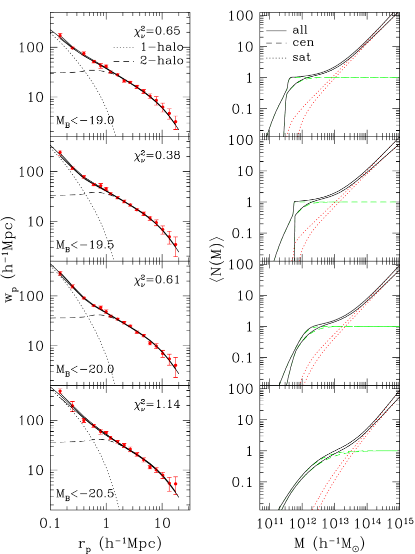
Figure 1.— HOD fits to $w_{p}(r_{p})$ (left) and the mean occupation functions (right) for DEEP2 galaxy samples. In each $w_{p}(r_{p})$ panel, overplotted on the data points are the range of lines predicted from models with $\Delta\chi^{2}<1$ (the reduced $\chi^{2}$ from the best fit is labeled in each panel). The one-halo (dotted line) and two-halo (dashed line) terms from the best-fit model are also plotted for illustration. In each $\langle N(M)\rangle$ panel, the envelopes of mean occupation functions from models with $\Delta\chi^{2}<1$ are plotted and the total mean occupation function (solid line) is decomposed into contributions from central (dashed line) and satellite (dotted line) galaxies.

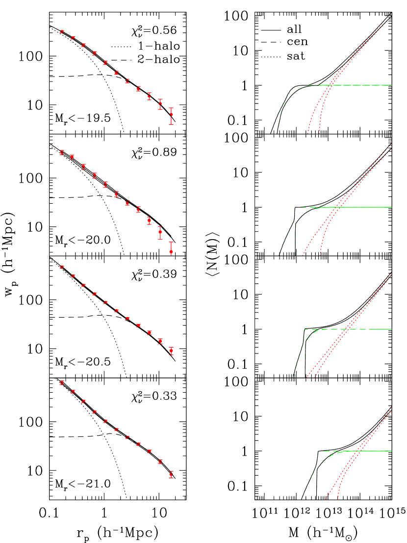
Figure 2.— Similar to Fig. 1, but for SDSS galaxy samples.

4.1. Results for DEEP2 Galaxies

The modeling results for the four DEEP2 luminosity threshold samples are shown in Figure 1. In each of the left panels, lines from model predictions are plotted together with the $w_{p}(r_{p})$ data points. All fits are excellent. With five parameters (one of which is largely determined by the mean galaxy density once the other four are specified), this success may seem unsurprising. However, it is worth noting that the combination of the CDM halo distribution (fixed by our assumed cosmology) and an HOD model cannot fit arbitrary functions — this is a physically constrained model with vastly less freedom than, say, a 4th-order polynomial. Our HOD fits self-consistently produce the two-point correlation function both on small scales and on large scales. On small scales, the two-point correlation function reflects how galaxies are spatially distributed inside halos. On large scales (e.g., $\sim 10h^{-1}{\rm Mpc}$), the galaxy two-point correlation function is simply the matter correlation function multiplied by a constant (i.e., the square of the scale-independent galaxy bias factor). Our HOD model nicely reproduces the large-scale shape of $w_{p}(r_{p})$, which indicates that the matter power spectrum we use has the correct shape on these scales.

The central solid line corresponds to the best-fit model and is bounded by two solid lines, which are the envelopes of predictions from models with $\Delta\chi^{2}<1$. As we do not have the full error covariance matrix, these should only be interpreted as indicative of the associated 1-$\sigma$ uncertainty. The best-fit line is decomposed into contributions from the one-halo term (intra-halo galaxy pairs; dotted lines) and two-halo term (inter-halo galaxy pairs; dashed lines), which dominate on small and large scales, respectively. The transition from the one-halo term to the two-halo term causes an inflection in $w_{p}(r_{p})$, leading to departures from a pure power law that are observed for both low redshift galaxies (e.g., Zehavi et al., 2004; Hawkins et al., 2003) and high-redshift galaxies (e.g., Ouchi et al., 2005; Lee et al., 2006). If the transition scale is defined as the scale where the two contributions to $w_{p}(r_{p})$ are equal, we find that it increases from $\sim$0.4$h^{-1}{\rm Mpc}$ to $\sim$0.6$h^{-1}{\rm Mpc}$ as the luminosity threshold of galaxies increases, a manifestation that more luminous galaxies reside in more massive halos.

The mean occupation functions for the four DEEP2 samples are shown in the right panels of Figure 1. The mean occupation function for all galaxies in the sample is decomposed into that for central galaxies and that for satellites. For each mean occupation function, we plot the envelope from models with $\Delta\chi^{2}<1$. It can be clearly seen that the mean occupation function shifts to higher halo mass as the luminosity of galaxies increases. In general, a low-mass cutoff in the satellite mean occupation function (which is usually neglected in the simple three-parameter model) is required by the DEEP2 $w_{p}(r_{p})$ data for a good model fit. The best-fit models for the two brighter samples have a shallow cutoff profile in $\langle N_{\rm cen}\rangle$. For the two fainter samples, the inferred cutoff profile in $\langle N_{\rm cen}\rangle$ can be either sharp or shallow, which leads to the kink seen in the envelope of $\langle N_{\rm cen}\rangle$ for models with $\Delta\chi^{2}<1$. The general trend that the central galaxy cutoff profile is better constrained for brighter galaxies reflects the fact that the halo mass function and bias factor change steeply toward the high mass end, although the residual redshift-space distortion [because of $w_{p}(r_{p})$ being derived from a finite projection] could artificially increase the shallowness of the cutoff profile (J. L. Tinker, private communication).

We note that the constraints on the HOD models can be further strengthened by enforcing the condition that at any halo mass the mean occupation number for central or satellite galaxies in a sample with lower luminosity threshold is always higher than that for galaxies in a sample with higher luminosity threshold. A full implementation of this would require modeling the data from all galaxy samples simultaneously, and there would be strong correlations among mean occupation functions of different samples. Here we choose to model each sample individually. To roughly account for the above condition, we drop some models that are in apparent conflict. Specifically, the mean occupation functions of satellites for the $M_{B}$$<$$-19.0$ sample from a small fraction of models have a cutoff at much higher mass than those for the $M_{B}$$<$$-19.5$ sample, which is not realistic. We therefore only keep models for the $M_{B}$$<$$-19.0$ sample with a satellite cutoff mass of $M_{0}$$<$$10^{12}h^{-1}M_{\odot}$ for the following discussions. We note that the above consistency condition is automatically satisfied by adopting the CLF method, with the HOD of each sample obtained by integrating the CLF over halo mass, although to reach a similar level of flexibility in the HOD we use here, more parameters need to be introduced in the CLF.

The high-mass end slopes $\alpha$ for mean occupation functions of satellites are found to be $0.89_{-0.34}^{+0.23}$, $0.97_{-0.11}^{+0.11}$, $1.08_{-0.06}^{+0.05}$, and $1.27_{-0.12}^{+0.12}$ in order of increasing luminosity threshold, where each value is quoted as the mean with error bars from the central 68.3% of the marginalized distribution (i.e., 1–$\sigma$ range). Although the value for the most luminous sample is slightly larger, all values are close to unity, which agrees with predictions of galaxy formation models (e.g., Kravtsov et al., 2004; Zheng et al., 2005).

We note that the best-fit HOD model for the brightest DEEP2 sample ($M_{B}<-20.5$) has a larger $\chi^{2}$ than those of the other samples. Much of the difference between the model and the data happens on small scales ($r_{p}\lesssim 0.5h^{-1}{\rm Mpc}$). On these scales, the raw measurements of $w_{p}(r_{p})$ are affected by the undersampling of galaxies caused by the slitmask target selection algorithm, and they are corrected by using the mock galaxy catalogs of Yan et al. (2004) (Coil et al., 2006a). In general, the correction increases the amplitude and the slope of $w_{p}(r_{p})$ on small scales by a small amount. As a test of the robustness of our HOD results to this correction, we perform an MCMC run with the uncorrected $w_{p}(r_{p})$ data for this sample and find $\chi^{2}/{\rm d.o.f.}=0.75$. The inferred HOD therefore seems to be robust against such a correction — there is almost no change, except for a slight decrease in the number of satellite galaxies in low-mass halos to account for the slightly reduced amplitude and slope of the uncorrected $w_{p}(r_{p})$. The slitmask correction could in principle be improved by using catalogs generated according to the best-fit HOD model and iterating the correction and model fitting a couple of times. However, given the robustness of the best-fit HOD under the adopted parameterization, we do not intend to perform such iterations in this paper.

We also tried to fit the data with a more flexible HOD parameterization, which uses a spline line for the satellite mean occupation function (similar to what is used in Fig.19c of Zehavi et al. 2005). We found that the HOD is adjusted to fit almost every feature in $w_{p}(r_{p})$, and the modeling may result in solutions that are not seen in galaxy formation models. For instance, for the brightest $M_{B}<-20.5$ sample, the best-fit satellite mean occupation function has an inflection and flattens out toward the low halo mass end, which allows it to fit the high amplitude and steep slope of $w_{p}(r_{p})$ on small scales that are vulnerable to slitmask corrections. Therefore, we conclude that this more flexible HOD parameterization might be “over fitting” the data, and that to robustly interpret the present data does not require an HOD form more flexible than our five-parameter model.

4.2. Results for SDSS Galaxies

The modeling results for SDSS galaxies using the five-parameter model described in §3.2 are shown in Figure 2. To be concise, only the results of the samples that are most relevant to the evolution connection between DEEP2 and SDSS galaxies (see § 6) are plotted in this figure, although we perform HOD modeling for all SDSS samples with luminosity cuts ranging from $M_{r}=-18.0$ to $M_{r}=-22.0$ (see Table 1).

Unlike the DEEP2 samples, the cutoff profiles of $\langle N_{\rm cen}(M)\rangle$ for the SDSS samples are loosely constrained. This can be partly explained by noticing that in the mass range of $10^{11}$–$10^{12}h^{-1}M_{\odot}$, both the halo mass function and the halo bias factor at $z$$\sim$1 are steeper than those at $z$$\sim$0, and therefore the galaxy number density and the amplitude of the two-point correlation function at large scales lead to a better constraint in the cutoff profile for DEEP2 galaxies. We also note that complete freedom in $\sigma_{\log M}$ [eq. (2)] leads to a strong correlation between $M_{\rm min}$ and $\sigma_{\log M}$ in the sense that larger $M_{\rm min}$ corresponds to larger $\sigma_{\log M}$, which results in poor constraints on $M_{\rm min}$. We assign a prior $\sigma_{\log M}<0.5$, being conservative according to theoretical predictions (Zheng et al., 2005), for SDSS galaxy samples with luminosity threshold fainter than $L_{*}$ ($M_{r}^{*}$$=$$-20.44$).

The transition scales from one-halo term to two-halo term for SDSS samples are around $1h^{-1}{\rm Mpc}$, larger than those for DEEP2 galaxies. The cause of such a shift is that the one-halo term for SDSS galaxies appears to be shallower than that for DEEP2 galaxies, which again reflects the change in the slope of the halo mass function in the mass range probed by DEEP2 and SDSS galaxies (note that, for the halo definition we adopt, at a given mass the comoving sizes of halos at the two epochs are the same). This also explains why the departure of the two-point correlation function from a power law becomes more prominent at higher redshift (e.g., Zehavi et al. 2004; Zheng 2004; Kravtsov et al. 2004; Ouchi et al. 2005).

5. Comparisons of the HOD Modeling Results for DEEP2 and SDSS Galaxies

In this section, on the basis of the MCMC results presented in the previous section, we compare the HODs of DEEP2 and SDSS galaxies in detail.

5.1. The Central Galaxy Luminosity as a Function of Halo Mass

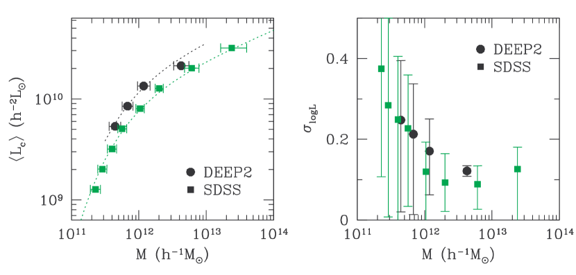
Figure 3.— Distribution of central galaxy luminosity as a function of halo mass. Left: Mean luminosity of central galaxies as a function of halo mass. Filled squares and circles are results for SDSS and DEEP2 galaxies, respectively. The error bars in halo mass indicate the 1–$\sigma$ range of the distribution from MCMC runs. Dotted lines are calculated using the fitting formula proposed by Vale & Ostriker (2006) with $L_{0}$ set to $2.8\times 10^{9}h^{-2}L_{\odot}$ (SDSS) and $4.3\times 10^{9}h^{-2}L_{\odot}$ (DEEP2) (see text for details). Right: Width of the distribution of central galaxy luminosity as a function of halo mass (see text for details).

As mentioned in § 3.2, the low-mass cutoff profile of the mean occupation function of central galaxies encodes information about the distribution of central galaxy luminosities in halos with mass close to the cutoff mass. By modeling the galaxy two-point correlation functions for samples with different luminosity thresholds, we can derive the distribution of the central galaxy luminosity as a function of halo mass. If the central galaxy luminosity $L_{c}$ in halos of fixed mass follows a log-normal distribution, as suggested by SA and SPH galaxy formation models (Zheng et al., 2005), then the mass scale $M_{\rm min}$ in equation (2) is the mass of halos for which the mean central galaxy luminosity $\langle L_{c}\rangle$ is simply the luminosity threshold of the galaxy sample (as shown in § 3.2). The left panel of Figure 3 shows the inferred $\langle L_{c}\rangle$–$M$ relation for DEEP2 galaxies and for SDSS galaxies. In the plot, absolute magnitudes are converted to luminosity in units of solar luminosity by using the Sun’s absolute magnitudes 4.76 in $r$–band (Blanton et al., 2003b) and 5.38 in $B$–band (Johnson AB magnitude).

The $\langle L_{c}\rangle$–$M$ relations look similar for the DEEP2 and SDSS galaxies except for an offset. At fixed halo mass, there is an offset of $\sim$1.4 in $\langle L_{c}\rangle$ between the DEEP2 and SDSS relations. However, given that the two samples are selected in different rest-frame bands, this offset does not necessarily imply that $z\sim 1$ DEEP2 galaxies are more luminous than $z\sim 0$ SDSS galaxies at a fixed halo mass. Alternatively, at fixed $\langle L_{c}\rangle$ there is an offset of $\sim 1.6$ in halo mass between the DEEP2 and SDSS samples. Similarly, the interpretation of such an offset is not immediately clear. In § 6 we attempt to establish a more meaningful evolutionary link between galaxies at the two epochs.

Because of a large range in galaxy luminosity, the SDSS samples probe the $\langle L_{c}\rangle$–$M$ relation over 2 orders of magnitude in halo mass, from $\sim$$2\times 10^{11}h^{-1}M_{\odot}$ to $\sim$$3\times 10^{13}h^{-1}M_{\odot}$, as shown in the left panel of Figure 3. We see that halos with higher mass host more luminous central galaxies at both $z\sim 1$ and $z\sim 0$. The plot shows that halos of Milky Way size ($\sim$$2\times 10^{12}h^{-1}M_{\odot}$) currently host central galaxies with mean luminosity about $L_{*}$ ($M_{r}^{*}=-20.44$, $L_{r}^{*}=1.20\times 10^{10}h^{-2}L_{\odot}$; Blanton et al. 2003b). Higher mass halos begin to host galaxy groups and clusters, so we expect that the $\langle L_{c}\rangle$–$M$ relation changes slope with halo mass. Indeed, the mean luminosity of central galaxies increases steeply with halo mass at the low-mass end and increases more slowly at the high-mass end, with the slope changing continuously from $\sim$2.5 to $\sim$0.3 over the mass range.

The $\langle L_{c}\rangle$–$M$ relation from the SDSS modeling results, whose slope becomes shallower toward higher halo mass, is in general agreement with results for local galaxies derived by other methods. Yang et al. (2005) infer the $\langle L_{c}\rangle$–$M$ relation in $b_{J}$ band through associating halos with galaxy groups identified in the 2dFGRS, and they find $\langle L_{c}\rangle\propto M^{2/3}$ for halos of $M\lesssim 10^{13}h^{-1}{\rm Mpc}$ and $\langle L_{c}\rangle\propto M^{1/4}$ for more massive halos. Using the X-ray masses of clusters/groups and the $K$-band luminosity of the brightest cluster galaxies in the Two Micron All Sky Survey (2MASS), Lin & Mohr (2004) find $\langle L_{c}\rangle\propto M^{0.26}$ for $M\gtrsim 2\times 10^{13}M_{\odot}$. By modeling the SDSS galaxy lensing data in McKay et al. (2001), Cooray & Milosavljević (2005) obtain the $\langle L_{c}\rangle$–$M$ relation for $M\lesssim 10^{13}M_{\odot}$, which can be approximated as $\langle L_{c}\rangle\propto M^{0.75}$. Vale & Ostriker (2004) present an empirical model for the relation between galaxy luminosity and halo mass by matching the galaxy luminosity function and halo/subhalo mass function (see also Vale & Ostriker 2006) and find that the mass luminosity relation can be well approximated by a double power law. Vale & Ostriker (2006) advocate a fitting formula of the following form:

$$\langle L_{c}\rangle=L_{0}\frac{(M/M_{c})^{a}}{[1+(M/M_{c})^{bk}]^{1/k}},$$ (6)

with $M_{c}=3.7\times 10^{9}h^{-1}M_{\odot}$, $a=29.78$, $b=29.5$, and $k=0.0255$. With these parameter values, $L_{0}$ is the mean galaxy luminosity in halos of mass $3.46\times 10^{11}h^{-1}M_{\odot}$. The relation is steep at low mass and becomes $\langle L_{c}\rangle\propto M^{0.28}$ at high mass. We find that this fitting formula provides a good description of our modeling results of the SDSS galaxies if $L_{0}=2.8\times 10^{9}h^{-2}L_{\odot}$ (see the dotted line for SDSS galaxies in the left panel of Fig. 3).

The DEEP2 galaxy samples we model probe the $\langle L_{c}\rangle$–$M$ relation at $z\sim 1$ over a smaller mass range, from $\sim$$4\times 10^{11}h^{-1}M_{\odot}$ to $\sim$$4\times 10^{12}h^{-1}M_{\odot}$. Central galaxies of luminosity $L_{*}$ ($M_{B}^{*}=-20.7$, $L_{B}^{*}=2.56\times 10^{10}h^{-2}L_{\odot}$, Willmer et al. 2006), which is slightly above the highest luminosity threshold we probe, tend to reside in halos a few times more massive than $L_{*}$ halos at $z\sim 0$. At $M<2\times 10^{12}h^{-1}M_{\odot}$, the shape of the $\langle L_{c}\rangle$–$M$ relation at $z\sim 1$ is consistent with that at $z\sim 0$. At higher halo masses, $\langle L_{c}\rangle$ appears to increase with $M$ slightly more slowly at $z\sim 1$ than at $z\sim 0$. The dotted line passing through the DEEP2 measurements in the left panel of Figure 3 is from the fitting formula in equation (6) with $L_{0}$ set to be $4.3\times 10^{9}h^{-2}L_{\odot}$.

In addition to the mean luminosity of central galaxies, with our modeling results, we can also study the width $\sigma_{\log L}$ of the distribution of central galaxy luminosity at a fixed halo mass [see eq. (4)]. The information is encoded in the width $\sigma_{\log M}$ of the cutoff profile of $\langle N_{\rm cen}(M)\rangle$ and the local slope $p$ of the $\langle L_{c}\rangle$–$M$ line — $\sigma_{\log L}=p\sigma_{\log M}/\sqrt{2}$ (see § 3.2). The results of the width of the central galaxy luminosity distribution are shown in the right panel of Figure 3, where a spline line passing through the $\langle L_{c}\rangle$–$M$ points is used to infer the local slope $p$ for the SDSS and DEEP2 samples, independently. The error bar on each point indicates the 1-$\sigma$ scatter in $\sigma_{\log L}$ (from its marginalized distribution) at the halo mass. In general, the scatter is not well-constrained by two-point correlation functions for low-luminosity samples, as the halo mass function and halo bias factor are not steep at the low-mass end. Therefore, we can remark only on general trends in the scatter. We find that at a fixed halo mass, the scatter $\sigma_{\log L}$ in the central galaxy luminosity for $z\sim 1$ DEEP2 galaxies is about 10%–20% higher than that for $z\sim 0$ SDSS galaxies, except for the brightest DEEP2 sample. For samples at both redshifts, there is a trend that $\sigma_{\log L}$ decreases with increasing halo mass, although the significance from the modeling results is marginal. In the mass range we can probe, $\sigma_{\log L}$ changes from $\sim 0.3$ to $\sim 0.1$ for both SDSS and DEEP2 galaxies. The value of $\sigma_{\log L}$ approaches a constant of $\sim 0.11$–0.12 at masses above $2\times 10^{12}h^{-1}M_{\odot}$ for both samples.

The decrease of $\sigma_{\log L}$ with increasing halo mass (except for the last SDSS data point), if true, is consistent with theoretical expectations (e.g., Zheng et al., 2005; Croton et al., 2006) in the halo mass range probed here. The last SDSS data point seems to show an increase but with large uncertainty. Although theoretical models also predict that $\sigma_{\log L}$ should increase with halo mass again at higher mass, it is at a mass much higher than probed here (e.g., $M>5\times 10^{13}h^{-1}M_{\odot}$). We note as well that the observed intrinsic scatter of the Tully-Fisher (Tully & Fisher, 1977) relation (e.g., Giovanelli et al., 1997), $\sim 0.20$–0.35 mag, implies $\sigma_{\log L}=$0.08–0.14 if one assumes that the circular velocity is a one-to-one indicator of halo mass. There is also a trend in the observed intrinsic scatter decreasing as the circular velocity increases, similar to what we see in our results. We speculate that the reason for the relatively large scatter in central galaxy luminosity for lower mass halos may be that the distribution of major star formation epochs is broad for these halos.

5.2. Relation Between Halo Mass Scales of Central and Satellite Galaxies

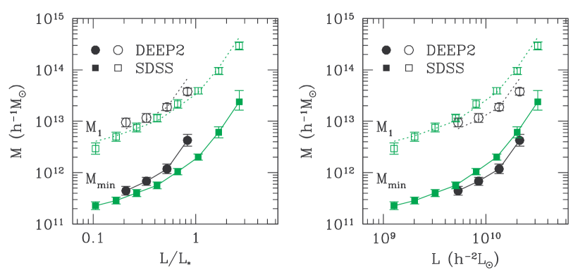
Figure 4.— Mass scales of halos hosting central galaxies and satellites as a function of galaxy luminosity. Left: Mass scales as a function of $L/L_{*}$. Filled symbols connected by solid lines are the relation between the characteristic minimum halo mass $M_{\rm min}$ and the luminosity threshold, and open symbols are that between $M_{1}$ and the luminosity threshold, where $M_{1}$ is the mass of a halo that on average hosts one satellite galaxy above the luminosity threshold. Dotted lines are obtained by multiplying the solid lines by a factor of 18 (SDSS) and 16 (DEEP2), respectively. Right: Same as the left panel, but the luminosity is expressed in units of solar luminosity.

In § 5.1 we determined the mass scales of central galaxies as a function of galaxy luminosity. We now focus on the halo occupation of satellite galaxies and the relation between the halo mass scales of central and satellite galaxies.

In our HOD parameterization, the parameter $M_{\rm min}$ can be interpreted as the characteristic minimum mass of the halo hosting a central galaxy above the luminosity threshold: $\langle N_{\rm cen}\rangle=0.5$ at $M_{\rm min}$ [see eq.( 2)]. For satellite galaxies, the characteristic halo mass scale $M_{1}$ is defined as the mass of a halo that on average can host one satellite galaxy above the luminosity threshold: $\langle N_{\rm sat}(M_{1})\rangle=1$ [note that $M_{1}$ is different from $M_{1}^{\prime}$ in eq.(5)]. In Figure 4 we show $M_{\rm min}$ and $M_{1}$ as a function of galaxy luminosity for DEEP2 and SDSS galaxies. In the left panel luminosity is relative to $L_{*}$ at each redshift, and in the right panel luminosity is in solar units. For central galaxies, the data points are essentially those in Figure 3 viewed at a different angle. As mentioned in § 5.1, the DEEP2 and SDSS galaxies are selected in different rest-frame bands, such that inferring evolution between the samples is complex. Comparing galaxies relative to $L_{*}$ at each redshift can roughly account for the different selections and the general dimming of galaxies since $z\sim 1$. The plot shows that the host halos of $z\sim 1$ $L_{*}$ galaxies are more massive than those of $z\sim 0$ $L_{*}$ galaxies, a trend of downsizing in terms of the host halo mass of “typical” galaxies with time since $z\sim 1$.

In Zehavi et al. (2005), the HOD modeling for SDSS galaxies reveals a relation $M_{1}\sim 23M_{\rm min}$. Because of the slightly different HOD parameterization, $M_{\rm min}$ and $M_{1}$ in our analysis do not correspond exactly to those in Zehavi et al. (2005). Our modeling results of the SDSS galaxies, as shown in Figure 4, can be expressed as $M_{1}\sim 18M_{\rm min}$. Zheng et al. (2005) present $M_{1}$–$M_{\rm min}$ relations in SA and SPH galaxy formation models for samples of galaxies above varying baryonic mass thresholds and find that the scaling factors are about 18 and 14 for the two models, respectively. Their definitions of $M_{\rm min}$ and $M_{1}$ are more consistent with the ones used here, and this may be the reason that our results here are in better agreement with the theoretical predictions of Zheng et al. (2005).

The $M_{1}$–$M_{\rm min}$ scaling relation for $z\sim 1$ DEEP2 galaxies is similar to that for $z\sim 0$ SDSS galaxies, as shown in Figure 4. The scaling factor is about 16, close to the value for SDSS galaxies. Dissipationless simulations in Kravtsov et al. (2004) show a weak trend of the scaling factor decreasing towards high redshift, which can be understood as the satellite galaxies not having enough time to merge with the central galaxies at higher redshift.

For both data sets, the scaling factor of the $M_{1}$–$M_{\rm min}$ relation has a trend of becoming smaller at the high-luminosity end. High luminosity satellite galaxies reside in massive halos. At any given redshift, massive halos form late and the accreted satellite galaxies do not have enough time to merge with the central galaxies. This effectively reduces the mass of the halos that on average host one satellite galaxy. Therefore, the effect of merging timescale may be the primary reason that the scaling factor decreases for very luminous galaxies.

From Figure 4, we can also see that at a fixed halo mass central galaxies are much more luminous than typical satellite galaxies for both DEEP2 and SDSS samples, with the difference being larger toward lower halo mass. This is a manifestation of a CLF bump caused by the central galaxy seen in galaxy formation models (Zheng et al. 2005).

5.3. Satellite Fraction

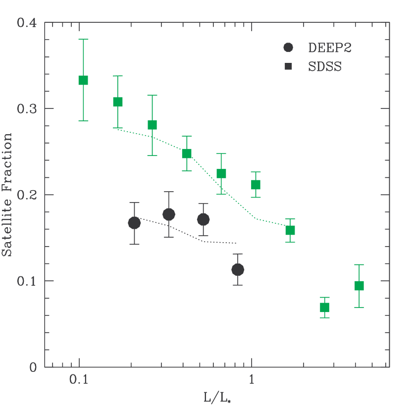
Figure 5.— Satellite fraction as a function of luminosity threshold for DEEP2 and SDSS galaxies. The luminosity threshold is expressed in units of $L_{*}$ at either redshift. Symbols show the mean value of the satellite fraction, and the error bars indicate the 1–$\sigma$ range of the marginalized distribution from MCMC runs. The dotted lines are calculated from interpolating the HOD parameters in Conroy et al. (2006), which are inferred through relating halos and subhalos in $N$-body simulations to galaxies.

A galaxy at a given luminosity can be either a central galaxy in a relatively lower mass halo or a satellite galaxy in a higher mass halo, with the former being much more probable (Zheng et al., 2005). Although at a fixed luminosity satellite galaxies are not dominant in number, they play a significant role in shaping the two-point correlation function of galaxies on small scales, where the one-halo term dominates. On these scales, galaxy pairs are composed of central-satellite and satellite-satellite pairs. Therefore, the two-point correlation function can provide strong constraints on the overall fraction of satellite galaxies.

Figure 5 shows the satellite fraction as a function of the luminosity threshold for DEEP2 and SDSS galaxy samples based on the MCMC runs, where the luminosity threshold is expressed in units of $L_{*}$. SDSS galaxies have a larger satellite fraction than DEEP2 galaxies. For example, $\sim$20% of $L\gtrsim L_{*}$ SDSS galaxies are satellite galaxies, compared to $\sim$10% of $L\gtrsim L_{*}$ DEEP2 galaxies. For both DEEP2 and SDSS galaxies, the satellite fraction tends to decrease as the luminosity threshold increases. For $L\gtrsim L_{*}$, the satellite fraction as a function of luminosity seems to drop more steeply. This trend with galaxy luminosity reveals that luminous galaxies are much more likely to be central galaxies in lower mass halos than satellite galaxies in higher mass halos.

Conroy et al. (2006) predict the evolution of the luminosity dependence of galaxy clustering for the redshift range $0<z<5$ by monotonically relating galaxy luminosities to the maximum circular velocity of halos and subhalos in $N$-body simulations. Their Table 2 lists the relevant HOD parameters at each redshift for various luminosity threshold samples, with different number densities. Our inferred HODs at $z\sim 1$ and $z\sim 0$ are in good agreement with their non-parametric results. The dotted lines in Figure 5 are satellite fractions calculated from interpolating the parameters in Conroy et al. (2006), which are consistent with our results in the relevant luminosity range. We note that satellite fractions, obtained here through HOD modeling of the two-point correlation function, can in principle be compared to those inferred through relating galaxy groups identified in the surveys (e.g., Gerke et al. 2005; Coil et al. 2006b for the DEEP2 survey and Berlind et al. 2006; Weinmann et al. 2006 for the SDSS survey) to dark matter halos for a consistency test.

On large scales, galaxy pairs have contributions from central galaxies paired with each other. Being lower in number, satellite galaxies do not contribute as much to the two-point galaxy correlation function on large scales as on small scales. However, applications that relate the large-scale galaxy bias factor (relative to dark matter) to the halo bias factor often neglect this small contribution from satellite galaxies, which can systematically affect the results on the inferred mass scale and number density of host halos. In the Appendix we quantify the systematic error resulting from the “one galaxy per halo” assumption using a simple HOD model.

6. Evolutionary Connections between DEEP2 Galaxies and SDSS Galaxies

Thus far, we have compared different aspects of the halo occupations of DEEP2 and SDSS galaxies, treating the results as “static” observations of the galaxy population at two different redshifts. We now attempt to establish an evolutionary link between galaxies at the two epochs to study the evolution of the (statistically) “same” galaxies with time. By “same” we mean a galaxy and its most massive progenitor.

HOD modeling converts observed galaxy clustering measurements to a relation between galaxy properties and their host dark matter halos. The formation and evolution of the halos themselves are dominated by gravity, which is well understood from theory and simulations. In principle, we know how the halo population at an earlier epoch evolves to that at a later epoch. Given the relationships between galaxies and halos at two different epochs, the galaxy populations at those epochs can then be linked through the growth of their halos.

In what follows, we implement this idea to study the evolution of central galaxies in the DEEP2 and SDSS samples. We first establish a relationship between $z\sim 0$ halo mass and progenitor halo mass at $z\sim 1$ in § 6.1. Using this relation and the HOD modeling results, in § 6.2 we link the $z\sim 0$ central galaxies and their progenitor central galaxies at $z\sim 1$ in terms of luminosity to measure the luminosity evolution of galaxies since $z\sim 1$. The stellar mass of a galaxy is perhaps a more fundamental physical parameter than luminosity and is more straightforward to interpret and compare to theoretical models. Therefore, in § 6.3, using the same halo mass relationship, we attempt to link central galaxies at the two redshifts in terms of stellar mass to study the growth of stellar mass as a function of host halo mass. From this we are able to draw tentative conclusions on galaxy evolution and star formation as a function of halo mass during the past $\sim$7 billion years. Finally, in § 6.4, using the stellar mass derived in § 6.3, we study how star formation efficiency depends on halo mass at the two redshifts.

6.1. Typical Growth of Halos from $z\sim$1 to $z\sim$0

To use our HOD results presented here, what we want to know is the mass of the $z\sim 1$ progenitor halo for each of the $z\sim 0$ host halos. A dark matter halo merger tree that traces the assembly history of halos serves this purpose well. We use the PINOCCHIO (PINpointing Orbit-Crossing Collapsed HIerarchical Objects) code developed by Monaco et al. (2002a; see also Monaco et al., 2002b; Taffoni et al., 2002) to predict the assembly history of dark matter halos. PINOCCHIO is based on Lagrangian perturbation theory and can generate synthetic catalogs of halos that include mass, position, velocity, merger history, and angular momentum. For the halo assembly history, predictions of PINOCCHIO are much more accurate than those based on the extended Press-Schechter formalism (EPS; Press & Schechter, 1974; Bond et al., 1991; Lacey & Cole, 1993). Compared to $N$–body simulations, PINOCCHIO can predict the average mass assembly history of halos to an accuracy of 10% or better (Li et al., 2005) with several orders of magnitude less computational time. Furthermore, unlike $N$–body simulations, which need expensive postprocessing to extract merger trees, PINOCCHIO directly outputs the merger history of each halo. We perform four realizations of PINOCCHIO in a $100{\rm Mpc}^{3}$ box and three realizations in a $50{\rm Mpc}^{3}$ box to probe assembly histories of halos with mass above and below $10^{12}M_{\odot}$, respectively. For these runs, the grid size is set to be $128^{3}$. The mass distribution of the $z\sim 1$ progenitor halos of the $z\sim 0$ halos is obtained in a series of $z\sim 0$ halo mass bins. The code does not include evolution of subhalos within parent halos, but it suffices for our purpose here as we focus only on central galaxies.

The results of the typical halo growth from $z\sim 1$ to $z\sim 0$ are presented in Figure 6$c$, which shows the relation between $M$, the mass of $z\sim 0$ halos, and $M_{\rm pro}$, the mass of their $z\sim 1$ progenitors. The solid line represents the mean mass of the progenitors, and the two dotted lines indicate the boundaries of the central 68.3% distribution of the progenitor mass as a function of the $z\sim 0$ halo mass. On average, lower mass halos grow earlier, in that more of their final mass is assembled by $z\sim 1$. The results show that a typical $z\sim 0$ halo with $M\sim 3\times 10^{11}h^{-1}M_{\odot}$ ($M\sim 10^{13}h^{-1}M_{\odot}$) has about 70% (50%) of its final mass in place at $z\sim 1$. We also use a merging tree code based on the (less accurate) EPS formalism and find that it generally predicts late growth for halos and leads to $\sim$15% lower masses of the $z\sim 1$ progenitors in the mass range we consider.

6.2. Luminosity Evolution

Figure 6.— Connection between DEEP2 galaxies and SDSS galaxies. Panels (a) and (d) show the mean luminosity of central galaxies as a function of halo mass at $z\sim$0 (SDSS) and $z\sim$1 (DEEP2). Panel (c) shows the relation between the mass $M$ of the $z\sim$0 halos and the mass $M_{\rm pro}$ of their $z\sim$1 progenitors. The solid line is the mean relation, and the dotted lines mark the central 68.3% of the distribution. Panels (a), (c), and (d) lead to a luminosity connection between DEEP2 galaxies and SDSS galaxies, which is shown in panel (b). The four dashed lines illustrate how this connection is established (see text for details).

The question we attempt to answer is, for galaxies of a given luminosity (e.g., $L_{*}$) at $z\sim 0$, what luminosity did their $z\sim 1$ progenitor galaxies have? We answer this question using the HOD results above and the $M_{\rm pro}$–$M$ relation shown in Figure 6$c$.

The $M_{\rm pro}$–$M$ relation links halos at $z\sim$1 to those at $z\sim$0. Together with the $\langle L_{c}\rangle$–$M$ relations at these two redshifts derived from DEEP2 and SDSS galaxies, which are plotted in Figure 6$d$ and Figure 6$a$, it enables a connection between DEEP2 and SDSS central galaxies. The dashed lines across the four panels of Figure 6 illustrate how such a connection is established. Figure 6$b$ shows the resultant connection between the $r$–band luminosity of $z\sim 0$ central galaxies and the $B$–band luminosity of their $z\sim 1$ progenitors. For example, the $z\sim 1$ progenitors of the $z\sim 0$ $L_{*}$ ($M_{r}^{*}=-20.44$; $L_{r}=1.20\times 10^{10}h^{-2}L_{\odot}$) central galaxies on average have a $B$–band luminosity of $M_{B}=-20.0$ ($L_{B}=1.34\times 10^{10}h^{-2}L_{\odot}$), less than $L_{*}$ at $z\sim 1$.

The above connection is between luminosities in two different rest-frame bands at the two redshifts. A more interesting comparison may be between luminosities in the same rest-frame band. The best way to achieve such a goal is to have galaxy samples observed in the same rest-frame band, which is not the case for samples analyzed here and is hard to achieve in general at different redshifts. However, we can obtain a rough connection by making a transformation between luminosities in the two bands. We use the publicly-available kcorrect code (Blanton et al., 2003a) to estimate the median $M_{B}$ values (where $B$ is a Bessell AB magnitude) for SDSS galaxies in a series of narrow $M_{r}$ bins, to facilitate comparison with $M_{B}$ samples in the DEEP2 data. Using the SDSS DR4 data and the same magnitude and redshift thresholds as Zehavi et al. (2005), we find that the median $M_{B}$ value for galaxies at a fixed $M_{r}$ is $M_{B}\simeq M_{r}+1$. Our transformation implies that $z\sim 0$ $L_{r}^{*}$ galaxies have a median $L_{B}\sim 8.0\times 10^{9}h^{-2}L_{\odot}$. On average their $z\sim 1$ progenitors have $M_{B}=-20.0$ (Fig. 6$b$), i.e., $L_{B}=1.34\times 10^{10}h^{-2}L_{\odot}$. It is not entirely surprising that their progenitor galaxies are more luminous, as stars fade as they age. Using the Bruzual & Charlot (2003) model, we find that the amount of passive luminosity evolution at a fixed time interval depends on the age of the stellar population, in the sense that younger populations fade more. This is related to the fact that luminous massive stars have a shorter lifetime. For a stellar population with 0.2–1 solar metallicity, which forms its stars in a single instantaneous burst at redshift $z=$1.5, 2, 2.5, or 3, its rest-frame $B$–band luminosity would decrease by about 1.8, 1.4, 1.2, or 1.0 mag, respectively, from $z=1$ to $z=0$. Using these values as an estimate, a $z\sim 1$ progenitor central galaxy would have $L_{B}\sim$2.6–5.3$\times 10^{9}h^{-2}L_{\odot}$ (higher luminosity for stars forming at higher redshift) if they were passively evolving to $z\sim 0$. This is fainter than the $z\sim 0$ central galaxies ($L_{B}\sim 8.0\times 10^{9}h^{-2}L_{\odot}$), which implies that additional stars must have been added to the system since $z\sim 1$, through star formation and/or galaxy mergers.

6.3. Stellar Mass Evolution

Figure 7.— Similar to Fig. 6, but in terms of mean stellar mass.

The connection between luminosities of local central galaxies and their progenitors provides interesting information on the evolution of the stellar component of galaxies from $z\sim 1$ to $z\sim 0$. However, a comparison in terms of stellar mass would be more informative and straightforward to interpret, as stellar mass is a more fundamental physical parameter than luminosity. As with luminosities, the ideal way to make this comparison is to construct stellar-mass-selected galaxy samples and to perform HOD modeling of the observed clustering of these samples, which we reserve for a future study. With the luminosity-selected samples used here, we use a simple estimation of stellar mass derived from the galaxy luminosity and color. While the correlation between stellar mass and galaxy luminosity can have a fair amount of scatter, we attempt here to extract useful information from the mean relation. The following analysis is presented as a proof of concept as to how one could attempt to study evolution of galaxies in terms of stellar mass and as a function of halo mass, and it serves only as a useful first-order approximation for analyses of stellar-mass-selected samples. With these caveats in mind, we proceed as follows.

For the DEEP2 galaxies, stellar masses are derived by Bundy et al. (2006) for the subset for which $K_{s}$-band imaging exists, assuming a Chabrier stellar initial mass function (IMF; (Chabrier, 2003)). An empirically-derived relation between rest-frame $UBV$ colors, redshift, and stellar mass is then used to estimate masses for the rest of the DEEP2 sample (C. N. A. Willmer, private communication). For the SDSS samples, we estimate the stellar mass from the $g-r$ color and the $r$–band luminosity using the relation given by Bell et al. (2003). The dominant source of uncertainty in estimating stellar mass using the above method is the IMF of stars (Bell & de Jong, 2001). The “diet” Salpeter IMF (Bell et al., 2003) is used for the SDSS galaxies. The effect of different IMFs is largely an offset in the estimated stellar mass. For example, stellar mass with the diet Salpeter IMF (Chabrier IMF) is 70% (50%) that with the Salpeter IMF. We multiply the DEEP2 stellar masses with the Chabrier IMF by a factor of 1.4 to convert them to a diet Salpeter IMF, so that stellar masses from both surveys can be compared.

Figure 8.— Mean stellar mass in $z\sim 0$ central galaxies and that in their $z\sim 1$ progenitors (top) and their ratio (bottom) as a function of the $z\sim 0$ host halo mass.

The mean stellar mass of galaxies and the scatter are calculated in a series of narrow luminosity bins. We can then convert the relation between central galaxy luminosity and halo mass to that between stellar mass of central galaxies and halo mass. With the present-day central galaxies and their progenitors at $z\sim 1$ linked through the $M_{\rm pro}$–$M$ relation, we recast Figures 6 in terms of stellar mass, which is shown in Figure 7. Here Figure 7$b$ shows the relation between the stellar mass of $z\sim 0$ central galaxies and that of the progenitors at $z\sim 1$. In Figure 8, the (arithmetic) mean stellar masses in central galaxies at $z\sim 0$ and those of their $z\sim 1$ progenitors as a function of the present-day halo mass are plotted, which allows an estimate of the average growth of central galaxy stellar mass from $z\sim 1$ to $z\sim 0$ as a function of halo mass. Limited by the luminosity range of the data, the halo mass range that can be probed is slightly greater than 1 order of magnitude. The bottom panel of Figure 8 shows the ratio of the mean stellar masses in the $z\sim 1$ progenitors and the $z\sim 0$ central galaxies as a function of the present-day halo mass, which is expected to be insensitive to the choice of the IMF. At $5\times 10^{11}h^{-1}M_{\odot}$, on average, a central galaxy had $\sim$20% of its present stellar mass in place at $z\sim 1$. The ratio gradually increases to $\sim$33% around $2\times 10^{12}h^{-1}M_{\odot}$ and is roughly constant up to the highest halo mass we can probe. For galaxies that reside in $2\times 10^{12}h^{-1}M_{\odot}$ halos (i.e., $z\sim 0$ $L_{r}^{*}$ galaxies), the increase in stellar mass from $z\sim 1$ appears to be consistent with the luminosity comparison presented in § 6.2 if most stars in their $z\sim 1$ progenitors do not form at a very high redshift and the luminosity is roughly proportional to stellar mass. As shown in Figure 7$c$, at $z\sim 1$, progenitor halos have already reached more than 50% of their total present-day mass. Therefore, in the mass range probed here, halos have most of their mass assembled by $z\sim 1$ but have most of their central galaxy stars assembled/formed more recently. The mass scale of 1–2$\times 10^{12}h^{-1}M_{\odot}$ for present-day halos appears to be a transition scale, below which a relatively larger fraction of stars have been added to the central galaxies during the period from $z\sim 1$ to $z\sim 0$.

In general, there are two processes that can add stellar components to central galaxies. One is star formation, and the other is galaxy merging, either merging of satellites with central galaxies or merging of central galaxies in different halos. The star formation includes that which occurs in the central galaxies and the star formation in the satellite galaxies that eventually merge onto central galaxies. If we know the halo occupation as a function of stellar mass at $z\sim 1$, we can evolve the subhalo and halo population at $z\sim 1$ to $z\sim 0$ using high-resolution $N$-body simulations or an analytic code (e.g., Zentner et al., 2005), assuming no star formation. Such a calculation would give the amount of stars acquired through mergers. The difference between the evolved stellar mass occupation and the true stellar mass occupation in halos of a given mass (inferred from $z\sim 0$ data) would tell us the amount of stars formed during the period from $z\sim 1$ to $z\sim 0$. While the samples we model are not well suited for such a sophisticated analysis, it is a goal we plan to pursue in future work.

The results presented in Figure 8 nevertheless allow us to place interesting limits on the amount of stars added to the present-day central galaxies by star formation and merging, in an average sense. As seen from Figures 6 and 8, for $z\sim 0$ halos with $M=5\times 10^{11}h^{-1}M_{\odot}$, their $z\sim 1$ progenitors have assembled $\sim$70% of the $z\sim 0$ mass while the progenitor central galaxies have $\sim$20% of the stellar mass in place. For low-mass halos, it is reasonable to assume that the stellar mass in the progenitor halo is dominated by those from central galaxies (see, e.g., Zheng et al. 2005). The progenitor halo therefore assembles the remaining $\sim$30% mass by $z\sim 0$ through smooth mass accretion and/or merging with one or more smaller halos. If the fraction of stellar mass inside this additional mass is the same as in the progenitor halo (i.e., smaller halos are assumed to have the same star-formation efficiency as the progenitor of the $5\times 10^{11}h^{-1}M_{\odot}$ halo), then at most $\sim$9% of the final stellar mass can be gained by this process. That is, the stellar mass in the progenitor galaxy and that in the smaller halos that could merge with it or the mass that is accreted can only amount to $\sim$30% of the final stellar mass in the $z\sim 0$ central galaxy. Therefore, for central galaxies in $z\sim 0$ halos with $M=5\times 10^{11}h^{-1}M_{\odot}$, $\sim$70% of the stars should form between $z\sim 1$ and $z\sim 0$.

Similar reasoning can be applied to higher mass halos, but one should keep in mind that the contribution of stellar mass in satellites increases with halo mass. For $z\sim 0$ halos with the highest mass we can probe ($M\lesssim 10^{13}h^{-1}M_{\odot}$, which host galaxy groups), satellite galaxies contribute a substantial amount of the stellar mass in the halo. The $z\sim 1$ progenitor of an average halo of this mass has assembled $\sim$54% of the total mass, and the progenitor central galaxy has $\sim$33% of its stellar mass assembled. Neglecting star formation, the progenitor central galaxy can merge with other central galaxies (with their total halo mass amounting to the remaining $\sim$46% of the $z\sim 0$ halo mass), and the total contribution to the stellar mass in the final $z\sim 0$ central galaxy from all the merged progenitor central galaxies would be at most 60%. Merging of satellites to the final central galaxy would make an additional contribution to the stellar mass. We crudely estimate this contribution as follows. In a halo, satellite galaxies are usually fainter than the central galaxy, and in galaxy groups, the brightest satellites are likely to be $\sim$1.6 mag ($\sim$25%) fainter than the central galaxies (i.e., the luminosity gap; see Milosavljević et al. 2006 and references therein). This means that even if all the brightest satellites in halos that are assembled into a $z\sim 0$ $10^{13}h^{-1}M_{\odot}$ halo are able to merge onto the final central galaxy, their contribution to the stellar mass is only about 25% of that from merging of central galaxies. Thus, the total stellar mass from merging of central galaxies and satellites may likely account for $\sim 60\%+60\%\times 25\%=75\%$ of that in the final central galaxies. The remaining $\sim$25% would then be the result of star formation between $z\sim 1$ and $z\sim 0$.

Figure 9.— Illustration of contributions to the average growth (since $z\sim 1$) of stellar mass of central galaxies residing in $z\sim 0$ halos, as a function of the $z\sim 0$ halo mass. See text for more details of the estimation based on the HOD modeling of galaxy clustering for the DEEP2 and SDSS galaxy samples. The top solid line would move up to be the dotted line after an upward correction of 25% for the DEEP2 stellar mass estimation (see text).

Using this same line of reasoning, we illustrate in Figure 9 the different contributions to the $z\sim 0$ central galaxy stellar mass in the halo mass range we are able to probe. In this plot, a linear interpolation in logarithmic halo mass, based on the above limits for the low- and high-mass ends, is assumed to estimate the contribution from satellite mergers. Based on these crude estimations, we find an interesting result: on average, a large fraction of stars in $z\sim 0$ central galaxies residing in low-mass halos formed since $z\sim 1$ (e.g., $\sim$70% for $5\times 10^{11}h^{-1}M_{\odot}$ halos), while only a small fraction of stars formed for central galaxies in high-mass halos (e.g., $\sim$25% for $\lesssim 10^{13}h^{-1}M_{\odot}$ halos) over the same period. This trend seems to be a manifestation of the so-called downsizing – a pattern in which the sites of active star formation shift from high-mass galaxies at early times to lower-mass systems at later epochs (e.g., Cowie et al., 1996; Juneau et al., 2005). If the trend continues to higher halo mass, beyond the luminosity range we probe in this paper, there may be no substantial star formation occurring between $z\sim 1$ and $z\sim 0$ in very massive halos.

Are these estimates reasonable? We can compare them to values obtained from the global cosmic star formation history (e.g., Madau et al. 1996), probed through different techniques. Using a recent compilation of data in Fardal et al. (2006), we estimate that about 40% of all the stars in the present universe formed between $z=1$ and $z=0$. Based on stellar mass estimates from the COMBO-17 survey, Borch et al. (2006) find that the total stellar mass density of the universe has roughly doubled since $z\sim 1$. These numbers are well bracketed by our values.

The mass dependence of star formation that we find here can also be compared with other results. We find that the stellar mass growth rate of central galaxies depends on the host halo mass. Since halo mass and central galaxy stellar mass are closely related, this implies that the growth rate depends on stellar mass itself. Jimenez et al. (2005) use spectroscopic modeling to infer the star formation histories of individual SDSS galaxies and derive the mean star formation history as a function of galaxy stellar mass. By integrating the fraction of stellar mass in the last 6.8 billion years as a function of stellar mass (sum of the dotted and all the solid lines in the top panel of their Fig.4), we find that for $z\sim 0$ galaxies with stellar mass $\sim 2\times 10^{10}M_{\odot}$, $\sim$70% of their stars formed between $z\sim 0.8$ and $z\sim 0$. This fraction drops to $\sim$40% for galaxies with a $z\sim 0$ stellar mass of $\sim 2\times 10^{11}M_{\odot}$. Using the star formation histories of SDSS galaxies estimated by Panter et al. (2006), which improves on the modeling in Jimenez et al. (2005), the above numbers become $\sim$60% and $\sim$25%. Our estimates show reasonable qualitative agreement with these results. It is worth noting that our method differs significantly from that of Panter et al. (2006), who use stellar population modeling of $z\sim 0$ SDSS galaxies with no reference to $z\sim 1$ galaxies, and do not use the clustering of either population. Our present analysis uses the population synthesis model only to obtain stellar mass-to-light ratios (not evolutionary ages), and our conclusions about stellar mass growth result from the HOD modeling of clustering at the two different redshifts. The agreement between the results from the two methods is therefore impressive.

Our results can also be compared with studies of the evolution of star formation rates (SFRs) as a function of stellar mass. Analyzing the AEGIS (All Wavelength Extended Groth Strip International Survey) data out to $z\sim 1$, Noeske et al. (2007a) find that star-forming galaxies form a distinct sequence with a power-law dependence of the SFR on the stellar mass (see also Noeske et al. 2007b). Converted to the “diet” Salpeter IMF, their result can be written as $SFR=3.6M_{\odot}~{}{\rm yr}^{-1}\times(M_{\rm star}/10^{10}M_{\odot})^{0.67}$ for $M_{\rm star}$ in the range of 1.4–14$\times 10^{10}M_{\odot}$ and $0.2<z<0.7$. If we parameterize the total stellar mass growth rate from both star formation and mergers as a power-law, $\dot{M}_{\rm star}=f(t)M_{\rm star}^{\gamma}$ (i.e., with a time-dependent normalization and time-independent power-law index), we can then solve for the mean relation averaged over $0<z<1$ utilizing the stellar mass connection between these two epochs (i.e., Fig. 7$b$). For $z\sim 0$ central galaxies with stellar mass in the range of 0.7–5$\times 10^{10}M_{\odot}$, we find that the mean growth rate of their stellar mass during the past $\sim$7Gyr is $\dot{M}_{\rm star}=2.9M_{\odot}~{}{\rm yr}^{-1}\times(M_{\rm star}/10^{10}M_{\odot})^{0.67}$. Compared with the SFR in the star formation phase mentioned above, it is interesting to notice that the general growth has the same dependence on the stellar mass but with only a $\sim$20% lower normalization, which suggests that, for these galaxies, star formation is the dominant mode of stellar mass growth and the star formation phase on average may occupy a substantial fraction of the 7 Gyr interval. Modeling galaxy clustering data in more redshift slices between $z\sim 1$ and $z\sim 0$ would lead to a better understanding of the implication of the general growth rate.

The numbers derived here should be taken as a first-order estimate, as we have performed an approximate calculation as a proof of concept. There are two limiting factors in the current data. As mentioned earlier, the samples used here are defined using galaxy luminosity, and modeling stellar mass-selected samples would be more appropriate for measuring the evolution of the stellar mass growth rate as a function of halo mass. The other complication is the different rest-frame color selections of the galaxies, in particular the effect that the DEEP2 samples used are not entirely volume limited for red galaxies (see § 2.1). This could lead to an underestimate of the mean stellar mass, as red galaxies have a higher stellar mass than blue galaxies at a given luminosity. Therefore, we may be overestimating the stellar mass evolution from $z\sim 1$ to $z\sim 0$. With smaller, volume-limited DEEP2 samples at a slightly lower redshift, we estimate that the fraction of galaxies missing in each DEEP2 sample is $\sim$10% and we also find that the mean stellar mass is likely to be underestimated by 20%–30%. This means that $\sim$25% more of the stellar mass could have been in place in the $z\sim 1$ progenitors than the numbers we quote here, which would move the line in the bottom panel of Figure 8 (and the lowest line in Fig. 9) up by $\sim$25%. Consequently, the top solid line in Figure 9 would shift upward to the place of the dotted line. The star formation contribution to the stellar mass growth at the lower (higher) halo mass end we probe would change from $\sim$70% ($\sim$25%) to $\sim$65% ($\sim$5%). However, despite these uncertainties, the general trend of the contribution to the stellar mass growth as a function of host halo mass remains the same. Therefore, the halo mass-dependent evolution trend inferred from the data is a robust result.

6.4. Evolution of the Star Formation Efficiency

Figure 10.— Mean fraction of baryons in host halos that are converted into stars in central galaxies for $z\sim 0$ (SDSS) and $z\sim 1$ (DEEP2) galaxies.

With the relation between stellar mass and halo mass at two epochs in hand, we now present the evolution of the star formation efficiency and discuss the implications.

Assuming that the baryon fraction in halos equals the mean baryonic fraction $f_{b}$ in the universe, for which we adopt the value 15.7% (see § 3.1), then stellar mass can be used to study the star formation efficiency as a function of halo mass at $z\sim 0$ and $z\sim 1$. Specifically, we associate a halo of mass $M$ with a baryon mass $M_{b}=f_{b}M$ and define $M_{\rm star}/M_{b}$ as the star-formation efficiency, where $M_{\rm star}$ is the stellar mass of the central galaxy in the halo. This star formation efficiency is, in essence, the value integrated from the redshift of formation to the epoch in consideration ($z\sim 1$ for DEEP2 galaxies and $z\sim 0$ for SDSS galaxies) and reflects the fraction of baryons associated with halos that have been converted to stars in the central galaxies by the given epoch. In practice, the baryon fraction in a halo may not equal the global fraction, due to various physical processes. For example, in a low-mass halo there may be a smaller fraction of baryons accreted because of the shallow potential well. Therefore, more accurately, the halo star formation efficiency defined here is the true star formation efficiency times the baryon accretion efficiency of the halo. Nevertheless, it is still an instructive quantity that can be interpreted as an apparent star formation efficiency. We note that by definition this efficiency does not include stars in satellite galaxies, whose contribution increases with halo mass (about a few percent at $5\times 10^{11}h^{-1}M_{\odot}$ and $\sim$40% at $10^{13}h^{-1}M_{\odot}$, according to the estimates in § 6.3).

Figure 10 shows this star formation efficiency, reflecting the fraction of baryons that are converted into stars at the two epochs. Both lines are calculated from the ratio of the arithmetic mean stellar mass of central galaxies in halos of a given mass to the average baryon mass associated with these halos. At $z\sim 0$, there is a characteristic mass scale of halos, $\sim 6\times 10^{11}h^{-1}M_{\odot}$, where the average conversion efficiency from baryons to stars in central galaxies reaches a maximal value. Even at this peak, only $\sim$27% of the baryons in the halo are converted into stars of the central galaxy. The star formation efficiency drops steeply at lower halo masses and declines more slowly at higher halo masses.

At $z\sim 1$, our inferred average conversion efficiency has a similar behavior to that at $z\sim 0$, but the overall conversion efficiency decreases and the peak is reached at a larger halo mass ($\sim$$10^{12}h^{-1}M_{\odot}$) with a value of $\sim$12%. While the absolute value of the efficiency depends on the IMF, the trend as a function of mass and thus the characteristic halo mass should not.

Shankar et al. (2006) infer the star formation efficiency at $z\sim 0$ by matching the observed galaxy stellar mass function with the theoretical halo mass function. Their result (see the dashed line in their Fig.5) is in a good agreement with ours on the trend of the efficiency with halo mass; our values are slightly lower than theirs but are well within the error bars. Mandelbaum et al. (2006) perform HOD modeling of galaxy-galaxy lensing for stellar mass-selected SDSS galaxy samples. The stellar mass in their study assumes the Kroupa (2001) IMF, which is about 30% lower than the diet Salpeter IMF we adopt here. With the IMF difference corrected, our estimate of the dependence of the $z\sim 0$ star formation efficiency on halo mass agrees well with their results (see their Table 3). After correcting for differences in the adopted IMF and halo definitions, in the relevant halo mass range our results at $z\sim 0$ and $z\sim 1$ also agree with those reported by Heymans et al. (2006) based on a weak gravitational lensing study of the Hubble Space Telescope GEMS (Galaxy Evolution from Morphologies and SED) survey. It is worth emphasizing that our results follow from the mass distribution of CDM halos and the galaxy assignment required to reproduce the observed clustering, while the galaxy lensing results are from direct measurements of the dark matter halos through their weak-lensing effects. The agreement between our results and the lensing results is therefore, again, impressive.

What determines the halo mass scale where the average conversion efficiency reaches a maximum? It could be star formation feedback or preheating. Mo et al. (2005) argue that present day halos less massive than $10^{12}h^{-1}M_{\odot}$ were embedded in pancakes of $M\sim 5\times 10^{12}h^{-1}M_{\odot}$ at $z\sim 2$, whose formation heats and compresses the gas, leading to a cooling time longer than the age of the universe at $z\lesssim 2$. Therefore, in halos below $10^{12}h^{-1}M_{\odot}$, there is not much cold gas available for star formation, which leads to the drop in the conversion efficiency. Our $z\sim 0$ mass scale is roughly consistent with their prediction. On the other hand, our results indicate that this halo mass scale shifts to a higher mass at $z\sim 1$. If true, preheating alone may not be sufficient to explain this mass scale. The intensity of star formation and the subsequent feedback as a function of halo mass and redshift may also be an important factor. The shift of the peak of star formation efficiency from high-mass halos to low-mass halos with time can be regarded as another manifestation of the downsizing pattern seen in star-forming galaxies. For both DEEP2 and SDSS galaxies, the drop of conversion efficiency above the characteristic halo mass could be in part due to the fact that we only consider stars in central galaxies, and in high-mass halos the stellar mass contributions from satellite galaxies can be substantial. In addition, in high-mass halos gas accretion becomes less efficient because of the high virial temperature. We note again that the stellar mass results presented here are shown mainly as a proof of concept and any conclusions based on these should be regarded as tentative.

7. Summary and Future Prospects

We perform HOD modeling of the projected galaxy two-point correlation functions $w_{p}(r_{p})$ for luminosity threshold samples of DEEP2 and SDSS galaxies at $z\sim 1$ and $z\sim 0$, respectively. The HOD modeling, which converts galaxy pair statistics to relations between galaxy properties and dark matter halos, reproduces well the galaxy correlation functions at these two redshifts, including the rise on small scales seen at $z\sim 1$.

We infer the relationship between central galaxy luminosity and halo mass at $z\sim 0$ and $z\sim 1$. We find that at both redshifts the mean central galaxy luminosity $\langle L_{c}\rangle$ increases with halo mass. In low-mass halos below $\sim 10^{12}h^{-1}M_{\odot}$, $\langle L_{c}\rangle$ increases more rapidly with halo mass, and the scatter in the central galaxy luminosity in halos of fixed mass appears larger, possibly reflecting the broad distribution of major star formation epochs in these halos. We find evolution in the HOD in that galaxies at a given halo mass are $\sim$1.4 times more luminous at $z\sim 1$ and for a given luminosity the halo mass is $\sim$1.6 times greater at $z\sim 0$, with the caution that luminosities of DEEP2 and SDSS are in different rest-frame bands. In addition, central $L_{*}$ galaxies are found to be in halos a few times more massive at $z\sim 1$ than at $z\sim 0$.

For both DEEP2 and SDSS galaxies, there exists a scaling relation between $M_{\rm min}$, the characteristic minimum mass of the halo that can host a central galaxy above a given luminosity threshold, and $M_{1}$, the mass scale of a halo that on average is able to host one satellite galaxy above the same luminosity threshold. There is little difference between the scaling relation at $z\sim 1$ ($M_{1}\simeq 16M_{\rm min}$) and that at $z\sim 0$ ($M_{1}\simeq 18M_{\rm min}$). The fraction of galaxies that are satellites decreases with increasing galaxy luminosity at both redshifts. At a fixed luminosity threshold (in units of $L_{*}$) SDSS galaxies have a larger satellite fraction than DEEP2 galaxies, e.g., $\sim$20% versus $\sim$10% for $L>L_{*}$ galaxies.

The ultimate goal in modeling galaxy clustering at different redshifts is to learn about galaxy formation and evolution. These HOD modeling results provide us with relationships between galaxies and dark matter halos at $z\sim 1$ and $z\sim 0$, spanning half the history of the universe. We use the typical growth of dark matter halos as determined from simulations to establish an evolutionary link between DEEP2 and SDSS galaxies and extract information about galaxy evolution over the last 7 billion years. We establish such a connection, on average, by linking $z\sim 0$ central galaxies to $z\sim 1$ central galaxies residing in the progenitor halos of the $z\sim 0$ halos. We relate the luminosities of $z\sim 0$ central galaxies to those of their $z\sim 1$ progenitors; however, the interpretation is complicated somewhat by the different rest-frame selection bands of SDSS and DEEP2 galaxies. As a proof of concept, we use stellar masses determined by galaxy color and luminosity to roughly estimate the evolution of the dependence of stellar mass on host halo dark matter mass. At $z\sim 1$ the mean fraction of baryons that have been converted into stars is below $\sim$15%, peaking at a halo mass of $10^{12}h^{-1}M_{\odot}$. At $z\sim 0$ this fraction is below $\sim$30% and the peak of the star formation efficiency is at a lower halo mass of $\sim 6\times 10^{11}h^{-1}M_{\odot}$. We find that, on average, the majority of stars in $z\sim 0$ central galaxies in low-mass halos (a few $\times 10^{11}h^{-1}M_{\odot}$) formed between $z\sim 1$ and $z\sim 0$, while only a small fraction of stars formed in central galaxies of halos as massive as $\sim 10^{13}h^{-1}M_{\odot}$. This reflects the downsizing pattern seen for star-forming galaxies as a function of stellar mass, shown now as a function of their host halo mass.

The stellar mass results presented here are preliminary, as the galaxy samples we model are defined by luminosity, not stellar mass. In addition, the SDSS and DEEP2 surveys have different rest-frame selection functions, which complicates comparing the results at the two redshifts. Ideally we would like to have stellar mass-selected galaxy samples at different redshifts from surveys that have the same rest-frame selection functions. While our results apparently agree with other studies in many aspects, we regard our conclusions on the details of the stellar mass evolution as tentative. Nevertheless, the halo mass-dependent evolution trend we infer appears to be robust, and the exercise serves as a starting point and guide for future work.

HOD modeling of galaxy clustering for stellar mass-selected samples at different redshifts would be a great tool for gaining insight on galaxy formation and evolution, and we plan to pursue this in future work. Unlike the simple estimates presented in this paper, which are based on a mean relationship between the final halo mass and progenitor halo mass, a comprehensive program would be more sophisticated. Halos at high redshift, populated with galaxies as a function of stellar mass in accordance with the HOD results, would serve as initial conditions. Then, assuming no star formation, these halos would be evolved forward in time to lower redshift, following the merging histories and satellite dynamics determined from simulations or analytic models. This method is similar to the semi-analytic galaxy formation model in merging of halos and dynamically evolving satellites, but here the initial conditions are set by the HOD modeling results. This method differs from semi-analytic models in that only dark matter evolution and dynamics, not baryon physics, are involved in the calculation. The difference between the evolved HOD and the HOD inferred from galaxy clustering at low redshift would then provide a wealth of information on star formation as a function of halo mass. For example, the contributions to stellar mass in central galaxies can be separated — what fractions are from star formation, from central galaxies in other halos that merge with them, and from minor mergers with satellite galaxies. We would also infer the average star formation history in satellite galaxies. If galaxy clustering is modeled at a series of redshifts, then the average continuous star formation history and the average stellar mass growth history from other modes (i.e., major and minor mergers) as a function of halo mass can be determined. Such empirically-derived results would shed light on the physics of galaxy formation, and comparisons with predictions of galaxy formation models would provide stringent tests for galaxy formation theory. An example of the effort starting along some of these lines is White et al. (2007), which uses $N$-body simulations in combination with HOD modeling of clustering to put constraints on merging of luminous galaxies from $z\sim 0.9$ to $z\sim 0.5$.

Additionally, the envisioned program may also help test the role of environment on galaxy formation and evolution. One of the main assumptions in the current HOD framework is that the galaxy content in halos depends only on the halo mass and is statistically independent of the halo’s larger scale environment. Gao et al. (2005) find in simulations a signature of age-dependent halo clustering (the so-called halo assembly bias, see also Croton et al. 2007; Jing et al. 2007; Harker et al. 2006; Wechsler et al. 2006; Wetzel et al. 2007; Zhu et al. 2006; Gao & White 2007). In general, the environmental effect on halo clustering is essentially negligible for halos above the nonlinear mass scale and becomes stronger for lower mass halos. With the method outlined above we may be able to test the effect of large-scale environment on galaxy evolution. It is likely that the environment-dependent halo clustering does not play a significant role in interpreting the observed galaxy clustering at high redshift due to the fast drop of the nonlinear mass (e.g., from $z=1$ to $z=0$, the nonlinear mass increases by a factor of $\sim$25, while halos only grow by a factor of about 2 in a large range of mass). When we passively evolve a high-redshift HOD, which is insensitive to the environment, to lower redshift, the environmental effect during the evolution can be fully taken into account. Comparing then the evolved HOD (which accounts for the environmental effect) with the HOD inferred from the low redshift data (which ignores the environmental effect) may provide insight on how environment shapes the HOD and determines properties of galaxies in low-mass halos, increasing the constraining power of galaxy clustering on galaxy formation processes.

Appendix A Bias related to the assumption of “one galaxy per halo”

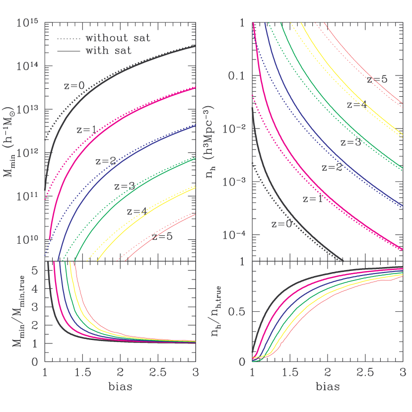
Figure 11.— Left: Comparison between the minimum mass $M_{\rm min}$ of the host halos under the assumption of one galaxy per halo (i.e., no satellite galaxies) and the true value at a measured galaxy bias factor for galaxy samples at different redshifts. The bottom panel shows the ratio of the $M_{\rm min}$ from one galaxy per halo to the true value. Right: Same as the left panels, but for comparisons between the inferred number densities of halos (see text for details).

Given a measured two-point correlation function for a galaxy population, HOD modeling is the ideal path to infer information about the host halos. However, this involves non-trivial modeling efforts, and therefore approximations are often used in the literature. One commonly-used method assumes that there is one galaxy per halo and connects galaxies to halos through the large-scale bias factor. This assumes that all galaxies in the sample are central galaxies, while in reality a small fraction are satellite galaxies. Using a simple HOD model, we quantify the resulting systematic bias in the inferred halo mass and the duty cycle of galaxies from this assumption.

We consider galaxy samples defined by a lower threshold in luminosity or stellar mass. The usual procedure associated with the “one galaxy per halo” assumption is as follows. The large-scale bias factor of galaxies is obtained from the ratio of the measured galaxy two-point correlation function and the theoretical matter two-point correlation function under the assumed cosmology. This large-scale bias factor is the same as that of halos above a mass threshold. Since for an assumed cosmology the latter is a known function of mass threshold (e.g., Mo & White 1996; Sheth et al. 2001; Tinker et al. 2005), the halo mass threshold $M_{\rm min}$ can be determined. The number density of halos above the mass threshold $M_{\rm min}$ can be inferred from the halo mass function (e.g., Sheth & Tormen 1999; Jenkins et al. 2001). The ratio of the observed galaxy number density to the inferred halo number density is used to determine the duty cycle of galaxies. More exactly, the “one galaxy per halo” assumption should be called “$f$ galaxy per halo,” where $f$ is a positive constant smaller than unity representing the duty cycle.

If satellite galaxies are taken into account, using the same galaxy bias factor measured from the data, a different $M_{\rm min}$ would be inferred. To see how large the difference is, we assume a simple mean occupation function to represent the “truth;” this model is the sum of a step function for central galaxies and a power law for satellite galaxies, $\langle N(M)\rangle=1+M/M_{1}$ for $M>M_{\rm min}$. Following galaxy formation model predictions (e.g., Kravtsov et al. 2004; Zheng et al. 2005) and HOD modeling results (e.g., this paper; Zehavi et al. 2005), we use $M_{1}=20M_{\rm min}$. The above $\langle N\rangle$ can have an overall normalization factor smaller than unity (duty cycle factor), and none of our results below change.

The bias factor $b$ for a given galaxy sample (in which all galaxies reside in halos of mass $M>M_{\rm min}$) can be calculated as

$$b(>M_{\rm min})=\left.\int_{M_{\rm min}}^{+\infty}dM\frac{dn}{dM}\langle N(M)\rangle b_{h}(M)\right/\int_{M_{\rm min}}^{+\infty}dM\frac{dn}{dM}\langle N(M)\rangle,$$ (A1)

where $dn/dM$ is the halo mass function and $b_{h}(M)$ is the bias factor of halos of mass $M$ (following Sheth & Tormen 1999). Solid lines in the top left panel of Figure 11 show the relation between $M_{\rm min}$ and $b(>M_{\rm min})$ at different redshifts. Assuming one galaxy per halo, the bias is calculated by replacing $\langle N(M)\rangle$ with unity in equation (A1). Dotted lines in the top left panel of Figure 11 show this relation. At a given bias factor (measured from the galaxy two-point correlation function), the value of $M_{\rm min}$ with the assumption of no satellite galaxies (dotted lines) is always higher than the “true” value (solid lines) because massive halos (with high halo bias) are weighted more as the number of satellites increases with halo mass. The bottom left panel of Figure 11 shows the ratio of the $M_{\rm min}$ from the “one galaxy per halo” method to the true value at each redshift, as a function of the galaxy bias. When the bias is high, the corresponding halos are in the exponential tail of the mass function and the weight from the satellite galaxies residing in massive halos is less significant, therefore, the value of $M_{\rm min}$ inferred from the approximate method approaches its true value. However, the difference increases for lower galaxy biases, corresponding to the shallower part of the halo mass function, and at higher redshift. For instance, at $z=0$, for a galaxy sample with $b=1.2$, the estimated $M_{\rm min}$ can be a factor of 2 higher than the true value.

The difference in the inferred values of $M_{\rm min}$ leads to a difference in the inferred number densities of halos above $M_{\rm min}$. The halo number density $n_{h}(>M_{\rm min})$ is calculated as

$$n_{h}(>M_{\rm min})=\int_{M_{\rm min}}^{+\infty}dM\frac{dn}{dM}.$$ (A2)

The right panels of Figure 11 compare the inferred (from “$f$ galaxy per halo”) and the true number densities of halos as a function of galaxy bias. For a given galaxy bias, the halo number density derived from the approximate $M_{\rm min}$ is always lower than the true value because without satellites in massive halos, a larger value of $M_{\rm min}$ is needed to reach the given bias factor. As with $M_{\rm min}$, the estimated halo number density approaches the true value for highly biased galaxy samples, while for low bias factors, the difference can again be substantial. For example, at $z=0$, the number density of host halos for galaxies with $b=1.2$ is underestimated by a factor of 2. As a consequence, the duty cycle (the fraction of halos hosting galaxies of that type) is overestimated by using the underestimated halo number density.

For galaxy samples defined by a lower threshold (e.g. in luminosity), Figure 11 can be used to better estimate the minimum host halo mass and number density from the measured galaxy bias value, instead of assuming one galaxy per halo.

References

- Abazajian et al. (2005) Abazajian, K., et al. 2005, ApJ, 625, 613
- Adelberger et al. (2005a) Adelberger, K. L., Erb, D. K., Steidel, C. C., Reddy, N. A., Pettini, M., & Shapley, A. E. 2005a, ApJ, 620, L75
- Adelberger et al. (2005b) Adelberger, K. L., Steidel, C. C., Pettini, M., Shapley, A. E., Reddy, N. A., & Erb, D. K. 2005b, ApJ, 619, 697
- Allen et al. (2005) Allen, P. D., Moustakas, L. A., Dalton, G., MacDonald, E., Blake, C., Clewley, L., Heymans, C., & Wegner, G. 2005, MNRAS, 360, 1244
- Bell & de Jong (2001) Bell, E. F., & de Jong, R. S. 2001, ApJ, 550, 212
- Bell et al. (2003) Bell, E. F., McIntosh, D. H., Katz, N., & Weinberg, M. D. 2003, ApJS, 149, 289
- Bell et al. (2005) Bell, E. F., et al. 2005, ApJ, 625, 23
- Benson et al. (2002) Benson, A. J., Lacey, C. G., Baugh, C. M., Cole, S., & Frenk, C. S. 2002, MNRAS, 333, 156
- Berlind & Weinberg (2002) Berlind, A. A. & Weinberg, D. H. 2002, ApJ, 575, 587
- Berlind et al. (2006) Berlind, A. A., et al. 2006, ApJS, 167, 1
- Blake et al. (2007) Blake, C., Collister, A., & Lahav, O. 2007, ArXiv e-prints, 704, arXiv:0704.3377
- Blanton et al. (2003a) Blanton, M. R., et al. 2003a, AJ, 125, 2348
- Blanton et al. (2003b) Blanton, M. R., et al. 2003b, ApJ, 592, 819
- Blanton et al. (2005) Blanton, M. R., et al. 2005, AJ, 129, 2562
- Bond et al. (1991) Bond, J. R., Cole, S., Efstathiou, G., & Kaiser, N. 1991, ApJ, 379, 440
- Borch et al. (2006) Borch, A., et al. 2006, A& A, 453, 869
- Bruzual & Charlot (2003) Bruzual, G., & Charlot, S. 2003, MNRAS, 344, 1000
- Bundy et al. (2006) Bundy, K., et al. 2006, ApJ, 651, 120
- Bullock et al. (2001) Bullock, J. S., Kolatt, T. S., Sigad, Y., Somerville, R. S., Klypin, A. A., Primack, J. R., Dekel, A. 2001, MNRAS, 321, 559
- Bullock, Wechsler, & Somerville (2002) Bullock, J. S., Wechsler, R. H., & Somerville, Rachel, S. 2002, MNRAS, 329, 246
- Chabrier (2003) Chabrier, G. 2003, PASP, 115, 763
- Cimatti et al. (2006) Cimatti, A., Daddi, E., & Renzini, A. 2006, A&A, 453, L29
- Coil et al. (2006a) Coil, A. L., Newman, J. A., Cooper, M. C., Davis, M., Faber, S. M., Koo, D. C., & Willmer, C. N. A. 2006a, ApJ, 644, 671
- Coil et al. (2006b) Coil, A. L., et al. 2006b, ApJ, 638, 668
- Colless et al. (2001) Colless, M., et al. 2001, MNRAS, 328, 1039
- Conroy et al. (2006) Conroy, C., Wechsler, R. H., & Kravtsov, A. V. 2006, ApJ, 647, 201
- Cooray & Sheth (2002) Cooray, A,, & Sheth, R. 2002, Phys. Rep., 372, 1
- Cooray (2005) Cooray, A. 2005, MNRAS, 364, 303
- Cooray (2006) Cooray, A. 2006, MNRAS, 365, 842
- Cooray & Milosavljević (2005) Cooray, A., & Milosavljević, M. 2005, ApJ, 627, L85
- Cooray & Ouchi (2006) Cooray, A., & Ouchi, M. 2006, MNRAS, 369, 1869
- Cowie et al. (1996) Cowie, L. L., Songaila, A., Hu, E. M., & Cohen, J. G. 1996, AJ, 112, 839
- Croton et al. (2006) Croton, D. J., et al. 2006, MNRAS, 365, 11
- Croton et al. (2007) Croton, D. J., Gao, L., & White, S. D. M. 2007, MNRAS, 374, 1303
- Daddi et al. (2003) Daddi, E., Röttgering, H. J. A., Labbe, I., Rudnick, G., et al. 2003, ApJ, 588, 50
- Davis et al. (2003) Davis, M., et al. 2003, Proc. SPIE, 4834, 161, ArXiv Astrophysics e-prints, arXiv:astro-ph/0209419
- Davis, Gerke, & Newman (2004) Davis, M., Gerke, B. F., & Newman, J. A. 2004, In Proceedings of ”Observing Dark Energy: NOAO Workshop”, Mar 18-20, 2004, ArXiv Astrophysics e-prints, arXiv:astro-ph/0408344
- Eisenstein & Hu (1998) Eisenstein, D. J., & Hu, W. 1998, ApJ, 496, 605
- Eisenstein et al. (2001) Eisenstein, D. J., et al. 2001, AJ, 122, 2267
- Erb et al. (2006a) Erb, D. K., Steidel, C. C., Shapley, A. E., Pettini, M., Reddy, N. A., & Adelberger, K. L. 2006a, ApJ, 646, 107
- Erb et al. (2006b) Erb, D. K., Steidel, C. C., Shapley, A. E., Pettini, M., Reddy, N. A., & Adelberger, K. L. 2006b, ApJ, 647, 128
- Faber et al. (2003) Faber, S., et al. 2003, Proc. SPIE, 4841, 1657
- Fardal et al. (2006) Fardal, M. A., Katz, N., Weinberg, D. H., & Davé, R. 2006, MNRAS, submitted, ArXiv Astrophysics e-prints, arXiv:astro-ph/0604534
- Gao et al. (2005) Gao, L., Springel, V., & White, S. D. M. 2005, MNRAS, 363, L66
- Gao & White (2007) Gao, L., & White, S. D. M. 2006, MNRAS, 377, L5
- Gerke et al. (2005) Gerke, B. F., et al. 2005, ApJ, 625, 6
- Gilks, Richardson, & Spiegelhalter (1996) Gilks, W. R., Richardson, S., & Spiegelhalter, D. J. 1996, Markov Chain Monte Carlo in Practice (London: Chapman and Hall)
- Giovanelli et al. (1997) Giovanelli, R., Haynes, M. P., Herter, T., Vogt, N. P., da Costa, L. N., Freudling, W., Salzer, J. J., & Wegner, G. 1997, AJ, 113, 53
- Gunn et al. (1998) Gunn, J. E., et al. 1998, AJ, 116, 3040
- Gunn et al. (2006) Gunn, J., et al. 2006, AJ, 131, 2332
- Hamana et al. (2006) Hamana, T., Yamada, T., Ouchi, M., Iwata, I., & Kodama, T. 2006, MNRAS, 369, 1929
- Harker et al. (2006) Harker, G., Cole, S., Helly, J., Frenk, C., & Jenkins, A. 2006, MNRAS, 367, 1039
- Hawkins et al. (2003) Hawkins, E., et al. 2003, MNRAS, 346, 78
- Heavens et al. (2004) Heavens, A., Panter, B., Jimenez, R., & Dunlop, J. 2004, Nature, 428, 625
- Heymans et al. (2006) Heymans, C., et al. 2006, MNRAS, 371, L60
- Hildebrandt et al. (2005) Hildebrandt, H., et al. 2005, A&A, 441, 905
- Jannuzi & Dey (1999) Jannuzi B.T., Dey A., 1999, in ASP Conf. Ser. 191, Photometric redshifts and high redshift galaxies, ed. R.J. Weymann, L.J. Storrie-Lombardi, M. Sawicki & R.J. Brunner (San Francisco, ASP), 111
- Jenkins et al. (2001) Jenkins, A., Frenk, C. S., White, S. D. M., Colberg, J. M., Cole, S., Evrard, A. E., Couchman, H. M. P., & Yoshida, N. 2001, MNRAS, 321, 372
- Jimenez et al. (2005) Jimenez, R., Panter, B., Heavens, A. F., & Verde, L. 2005, MNRAS, 356, 495
- Jimenez et al. (2006) Jimenez, R., Bernardi, M., Haiman, Z., Panter, B., & Heavens, A. F. 2006, ApJ, submitted, ArXiv Astrophysics e-prints, arXiv:astro-ph/0610724
- Jing, Mo, & Börner (1998) Jing, Y. P., Mo, H. J., & Börner, G. 1998, ApJ, 494, 1
- Jing & Börner (1998) Jing, Y. P. & Börner, G. 1998, ApJ, 503, 37
- Jing, Börner, & Suto (2002) Jing, Y. P., Börner, G., & Suto, Y. 2002, ApJ, 564, 15
- Jing et al. (2007) Jing, Y. P., Suto, Y., & Mo, H. J. 2006, ApJ, 657, 664
- Juneau et al. (2005) Juneau, S., et al. 2005, ApJ, 619, L135
- Kravtsov et al. (2004) Kravtsov, A. V., Berlind, A. A., Wechsler, R. H., Klypin, A. A., Gottlöber, S., Allgood, B., & Primack, J. R. 2004, ApJ, 609, 35
- Kroupa (2001) Kroupa, P. 2001, MNRAS, 322, 231
- Lacey & Cole (1993) Lacey, C., & Cole, S. 1993, MNRAS, 262, 627
- Lee et al. (2006) Lee, K., Giavalisco, M., Gnedin, O. Y., Somerville, R., Ferguson, H., Dickinson, M., & Ouchi, M. 2006, ApJ, 642, 63
- Le Fevre et al. (2005) Le Fevre, O., et al. 2005, A&A, 439, 845
- Li et al. (2005) Li, Y., Mo, H. J., & van den Bosch, F. C. 2005, MNRAS, in press, ArXiv Astrophysics e-prints, arXiv:astro-ph/0510372
- Lin & Mohr (2004) Lin, Y.-T., & Mohr, J. J. 2004, ApJ, 617, 879
- Ma & Fry (2000) Ma, C., & Fry, J. N. 2000, ApJ, 543, 503
- Macciò et al. (2006) Macciò, A. V., Moore, B., Stadel, J., & Diemand, J. 2006, MNRAS, 156
- Madau et al. (1996) Madau, P., Ferguson, H. C., Dickinson, M. E., Giavalisco, M., Steidel, C. C., & Fruchter, A. 1996, MNRAS, 283, 1388
- Magliocchetti & Porciani (2003) Magliocchetti, M., & Porciani, C. 2003, MNRAS, 346, 186
- Mandelbaum et al. (2006) Mandelbaum, R., Seljak, U., Kauffmann, G., Hirata, C. M., & Brinkmann, J. 2006, MNRAS, 368, 715
- Matarrese et al. (1997) Matarrese, S., Coles, P., Lucchin, F., & Moscardini, L. 1997, MNRAS, 286, 115
- McKay et al. (2001) McKay, T. A., et al. 2001, ArXiv Astrophysics e-prints, arXiv:astro-ph/0108013
- Milosavljević et al. (2006) Milosavljević, M., Miller, C. J., Furlanetto, S. R., & Cooray, A. 2006, ApJ, 637, L9
- Mo & White (1996) Mo, H. J. & White, S. D. M. 1996, MNRAS, 282, 347
- Mo et al. (2005) Mo, H. J., Yang, X., van den Bosch, F. C., & Katz, N. 2005, MNRAS, 363, 1155
- Monaco et al. (2002a) Monaco, P., Theuns, T., & Taffoni, G. 2002, MNRAS, 331, 587
- Monaco et al. (2002b) Monaco, P., Theuns, T., Taffoni, G., Governato, F., Quinn, T., & Stadel, J. 2002, ApJ, 564, 8
- Moscardini et al. (1998) Moscardini, L., Coles, P., Lucchin, F., & Matarrese, S. 1998, MNRAS, 299, 95
- Moustakas & Somerville (2002) Moustakas, L. A., & Somerville, R. S. 2002, ApJ, 577, 1
- Nagai & Kravtsov (2005) Nagai, D., & Kravtsov, A. V. 2005, ApJ, 618, 557
- Navarro, Frenk, & White (1995) Navarro, J. F., Frenk, C. S., & White, S. D. M. 1995, MNRAS, 275, 56
- Navarro, Frenk, & White (1996) Navarro, J. F., Frenk, C. S., & White, S. D. M. 1996, ApJ, 462, 563
- Navarro, Frenk, & White (1997) Navarro, J. F., Frenk, C. S., & White, S. D. M. 1997, ApJ, 490, 493
- Noeske et al. (2007a) Noeske, K. G., et al. 2007a, ApJ, 660, 43
- Noeske et al. (2007b) Noeske, K. G., et al. 2007b, ApJ, 660, L47
- Oguri & Lee (2004) Oguri, M., & Lee, J. 2004, MNRAS, 355, 120
- Ouchi et al. (2004) Ouchi, M., et al. 2004, ApJ, 611, 685
- Ouchi et al. (2005) Ouchi, M., et al. 2005, ApJ, 635, L117
- Panter et al. (2006) Panter, B., Jimenez, R., Heavens, A. F., & Charlot, S. 2006, MNRAS, in press, ArXiv Astrophysics e-prints, arXiv:astro-ph/0608531
- Peacock & Smith (2000) Peacock, J. A., & Smith, R. E. 2000, MNRAS, 318, 1144
- Press & Schechter (1974) Press, W. H., & Schechter, P. 1974, ApJ, 187, 425
- Richards et al. (2002) Richards, G. T., et al. 2002, AJ, 123, 2945
- Riess et al. (2004) Riess, A. G., et al. 2004, ApJ, 607, 665
- Scoccimarro et al. (2001) Scoccimarro, R., Sheth, R. K., Hui, L., & Jain, B. 2001, ApJ, 546, 20
- Seljak (2000) Seljak, U. 2000, MNRAS, 318, 203
- Sheth et al. (2001) Sheth, R. K., Mo, H. J., & Tormen, G. 2001, MNRAS, 323, 1
- Sheth & Tormen (1999) Sheth, R. K. & Tormen, G. 1999, MNRAS, 308, 119
- Shankar et al. (2006) Shankar, F., Lapi, A., Salucci, P., De Zotti, G., & Danese, L. 2006, ApJ, 643, 14
- Smith et al. (2003) Smith R. E., et al. 2003, MNRAS, 341, 1311
- Spergel et al. (2003) Spergel, D. N., et al. 2003, ApJS, 148, 175
- Spergel et al. (2007) Spergel, D. N., et al. 2007, ApJS, 170, 377
- Springel et al. (2005) Springel, V., et al. 2005, Nature, 435, 629
- Stoughton et al. (2002) Stoughton, C., et al. 2002, AJ, 123, 485
- Strauss et al. (2002) Strauss, M. A., et al. 2002, AJ, 124, 1810
- Taffoni et al. (2002) Taffoni, G., Monaco, P., & Theuns, T. 2002, MNRAS, 333, 623
- Taylor & Babul (2001) Taylor, J. E., & Babul, A. 2001, ApJ, 559, 716
- Taylor & Babul (2004) Taylor, J. E., & Babul, A. 2004, MNRAS, 348, 811
- Tegmark et al. (2004) Tegmark, M., et al. 2004, Phys. Rev. D, 69, 103501
- Tinker et al. (2005) Tinker, J. L., Weinberg, D. H., Zheng, Z., & Zehavi, I. 2005, ApJ, 631, 41
- Tully & Fisher (1977) Tully, R. B., & Fisher, J. R. 1977, A&A, 54, 661
- Vale & Ostriker (2004) Vale, A., & Ostriker, J. P. 2004, MNRAS, 353, 189
- Vale & Ostriker (2006) Vale, A., & Ostriker, J. P. 2006, MNRAS, 371, 1173
- van den Bosch et al. (2003) van den Bosch, Frank, C., Yang, X. H., & Mo, H. J. 2003, MNRAS, 340, 771
- van den Bosch et al. (2005) van den Bosch, F. C., Tormen, G., & Giocoli, C. 2005, MNRAS, 359, 1029
- Wechsler et al. (2006) Wechsler, R. H., Zentner, A. R., Bullock, J. S., Kravtsov, A. V., & Allgood, B. 2006, ApJ, 652, 71
- Weinmann et al. (2006) Weinmann, S. M., van den Bosch, F. C., Yang, X., & Mo, H. J. 2006, MNRAS, 366, 2
- Wetzel et al. (2007) Wetzel, A. R., Cohn, J. D., White, M., Holz, D. E., & Warren, M. S. 2007, ApJ, 656, 139
- White et al. (2007) White, M., Zheng, Z., Brown, M. J. I., Dey, A., & Jannuzi, B. T. 2007, ApJ, 655, L69
- Willmer et al. (2006) Willmer, C., et al. 2006, ApJ, 647, 853
- Wolf et al. (2004) Wolf, C., et al. 2004, A&A, 421, 913
- Yan, Madgwick, & White (2003) Yan, R., Madgwick, D. S., & White, M. 2003, ApJ, 598, 848
- Yan et al. (2004) Yan, R., White, M., & Coil, A. L. 2004, ApJ, 607, 739
- Yang, Mo, & van den Bosch (2003) Yang, X. H., Mo, H. J., & van den Bosch, F. C. 2003, MNRAS, 339, 1057
- Yang et al. (2005) Yang, X., Mo, H. J., Jing, Y. P., & van den Bosch, F. C. 2005, MNRAS, 358, 217
- York et al. (2000) York, D. G., et al. 2000, ApJ, 120, 1579
- Zehavi et al. (2004) Zehavi, I., et al. 2004, ApJ, 608, 16
- Zehavi et al. (2005) Zehavi, I., et al. 2005, ApJ, 630, 1
- Zentner et al. (2005) Zentner, A. R., Berlind, A. A., Bullock, J. S., Kravtsov, A. V., & Wechsler, R. H. 2005, ApJ, 624, 505
- Zheng (2004) Zheng, Z. 2004, ApJ, 610, 61
- Zheng et al. (2005) Zheng, Z., et al. 2005, ApJ, 633, 791
- Zheng et al. (2007) Zheng, X. Z., Bell, E. F., Papovich, C., Wolf, C., Meisenheimer, K., Rix, H.-W., Rieke, G. H., & Somerville, R. 2007, ApJ, 661, L41
- Zhu et al. (2006) Zhu, G., Zheng, Z., Lin, W. P., Jing, Y. P., Kang, X., & Gao, L. 2006, ApJ, 639, L5