The XMM-Newton serendipitous survey

Abstract

Context. Recent results have revised upwards the total X-ray background (XRB) intensity below $\sim$10 keV, therefore an accurate determination of the source counts is needed. There are also contradicting results on the clustering of X-ray selected sources.

Aims. We have studied the X-ray source counts in four energy bands soft (0.5-2 keV), hard (2-10 keV), XID (0.5-4.5 keV) and ultra-hard (4.5-7.5 keV), to evaluate the contribution of sources at different fluxes to the X-ray background. We have also studied the angular clustering of X-ray sources in those bands.

Methods. AXIS (An XMM-Newton International Survey) is a survey of 36 high Galactic latitude XMM-Newton observations covering 4.8 deg² and containing 1433 serendipitous X-ray sources detected with 5-$\sigma$ significance. This survey has similar depth to the XMM-Newton catalogues and can serve as a pathfinder to explore their possibilities. We have combined this survey with shallower and deeper surveys, and fitted the source counts with a Maximum Likelihood technique. Using only AXIS sources, we have studied the angular correlation using a novel robust technique.

Results. Our source counts results are compatible with most previous samples in the soft, XID, ultra-hard and hard bands. We have improved on previous results in the latter band. The fractions of the XRB resolved in the surveys used in this work are 87%, 85%, 60% and 25% in the soft, hard, XID and ultra-hard bands, respectively. Extrapolation of our source counts to zero flux are not enough to saturate the XRB intensity. Only galaxies and/or absorbed AGN may be able contribute the remaining unresolved XRB intensity. Our results are compatible, within the errors, with recent revisions of the XRB intensity in the soft and hard bands. The maximum fractional contribution to the XRB comes from fluxes within about a decade of the break in the source counts ($\sim 10^{-14}$ cgs), reaching $\sim$50% of the total in the soft and hard bands. Angular clustering (widely distributed over the sky and not confined to a few deep fields) is detected at 99-99.9% significance in the soft and XID bands, with no detection in the hard and ultra-hard band (probably due to the smaller number of sources). We cannot confirm the detection of significantly stronger clustering in the hard-spectrum hard sources.

Conclusions. Medium depth surveys such as AXIS are essential to determine the evolution of the X-ray emission in the Universe below 10 keV.

1 Introduction

The X-ray background (Giacconi et al. Giacconi62 (1962)) is a testimony of the history of accretion power in the Universe (Fabian & Iwasawa FabianIwasawa99 (1999), Sołtan Soltan82 (1982)), and as such its sources and their evolution have attracted considerable attention (Fabian & Barcons FabianBarcons92 (1992)). Deep pencil-beam surveys (Loaring et al. Loaring05 (2005), Bauer et al. Bauer04 (2004), Cowie et al. Cowie02 (2002), Giacconi et al. Giacconi02 (2002), Hasinger et al. Hasinger01 (2001)) have resolved most ($\gse 90$%) of the soft (0.5-2 keV) XRB into individual sources. Most of these turn out to be unobscured and obscured Active Galactic Nuclei (AGN), while at the fainter fluxes a population of ”normal” galaxies starts to contribute significantly to the source counts (Hornschemeier et al. Hornschemeier03 (2003)). At higher energies the resolved fraction is smaller (Worsley et al. Worsley04 (2004)): 50% between 4.5 and 7.5 keV, and less than 50% between 7.5 keV and 10 keV. Models for the XRB based on the Unified Model for AGN reproduce successfully its spectrum with a combination of unobscured and obscured AGN, the later being the dominant population (Setti & Woltjer Setti89 (1989), Gilli et al. Gilli01 (2001)). Recent hard X-ray AGN luminosity function results (Ueda et al. Ueda03 (2003), La Franca et al. LaFranca05 (2005)) show that such simple models need considerable revision, with lower absorbed AGN fraction at higher luminosities and luminosity dependent density evolution of the hard X-ray AGN luminosity.

The fainter sources from deep surveys do not contribute much to the final XRB intensity, and are often too faint optically and in X-rays to be studied individually. Stacking of X-ray spectra is a valuable tool in these circumstances (Worsley et al. Worsley06 (2006), Civano, Comastri & Brusa Civano05 (2005)), but only average properties can be studied in this fashion, missing all the diversity in the nature of the sources necessary to account for the XRB. Wide shallow surveys over a large portion of the sky (Schwope et al. Schwope00 (2000), Della Ceca et al. DellaCeca04 (2004), Ueda et al. Ueda03 (2003)) allow detecting minority populations and studies of sources on an individual basis, and serve as a framework against which to study and detect evolution, but again with only a minor contribution to the XRB.

Medium depth wide-band surveys combining many sources with relatively wide sky coverage ( Hasinger et al. Hasinger07 (2007), Pierre et al. Pierre04 (2004), Barcons et al. Barcons02 (2002), Baldi et al. Baldi02 (2002)) have the potential to provide many of the missing pieces of the XRB/AGN puzzle, since most (30-50%) of the XRB below 10 keV comes from sources at intermediate fluxes (Fabian & Barcons FabianBarcons92 (1992), Barcons, Carrera & Ceballos Barcons06a (2006)), and the optical and X-ray spectra of many sources can be studied individually (e.g. Mateos et al. Mateos05 (2005)). Furthermore, extensive XMM-Newton source catalogues are available (1XMM -SSC SSC03 (2003)-), and even larger ones will be available in the near future (2XMM,$\ldots$), which, since they are constructed from serendipitous sources in typical public XMM-Newton observations, are themselves medium flux surveys. The exploitation of the full potential of these catalogues depends on the results from “conventional” smaller scale medium flux surveys such as those above and the one presented here.

Since AGN are the dominant population at medium and low X-ray fluxes, and X-ray selected AGN are known to cluster strongly (Yang et al. Yang06 (2006), Gilli et al. Gilli05 (2005), Mullis et al. Mullis04 (2004), Carrera et al. Carrera98 (1998)), it is interesting to investigate the angular clustering of X-ray sources, which can be performed without resorting to expensive ground-based spectroscopy. Angular correlation can be translated into spatial clustering via Limber’s equation (Peebles Peebles80 (1980)), if the luminosity function of the populations involved is known from other surveys. Several studies have investigated the angular clustering in the soft and hard bands in scales of tens-hundreds of arcsec to degrees, with varying success in the detection of signal. Angular clustering has been detected in the soft band (Gandhi et al. Gandhi06 (2006), Basilakos et al. Basilakos05 (2005), Akylas et al. Akylas00 (2000), Vikhlinin & Forman Vikhlinin95 (1995)) with different values of the clustering strength. Angular clustering in the hard band has evaded detection in some cases (Gandhi et al. Gandhi06 (2006), Puccetti et al. Puccetti06 (2006)), but not in others (Yang et al. Yang03 (2003), Basilakos et al. Basilakos04 (2004)), in the latter cases finding clustering strengths marginally compatible with the observed spatial clustering of optical and X-ray AGN.

We present here a medium X-ray survey which includes 1433 serendipitous sources over 4.8 deg²: AXIS (An X-ray International Survey). This survey was undertaken under the auspices of the XMM-Newton Survey Science Centre (SSC). In this paper we present the source catalogue (Section 2), overall X-ray spectral properties (Section 3), number counts (Section 4, where some other samples have also been used), fractional contribution to the XRB (Section 5), and angular clustering properties (Section 6). Overall results are summarised in Section 7. In a forthcoming paper (Barcons et al. Barcons06b (2007)) we present the optical identifications of a subsample of AXIS, which we have called the XMM-Newton Medium Survey (XMS). In this paper we will use cgs as a shorthand for the cgs system units for the flux: erg cm^-2 s^-1.

2 The X-ray data

Table 1: Basic data for the 36 fields in the AXIS survey: including the target name, the XMM-Newton OBS_ID number of the pn dataset used, the R.A. and Dec. of the field centre, the “clean” exposure time and the filter used for the pn camera, the Galactic column density in the direction of the field (Dickey & Lockman 1990), and, when applicable, the centre and radius of the circular target exclusion area, the width of the OOT exclusion area, and the centre and radius of an additional exclusion area around bright/extended sources.

Target name	OBS_ID	R.A.	Dec	Texp	Filter	$N_{\rm H,Gal}$	R.A.	Dec.	R	OOT	R.A.	Dec.	R’
		(J2000)	(J2000)	(s)		($10^{20}$ cm-2)	(J2000)	(J2000)	($"$)	($"$)	(J2000)	(J2000)	($"$)
A2690	0125310101	00:00:30.30	$-$25:07:30.00	21586.7	Medium	1.84	00:00:21.2	$-$25:08:12.18	20	0	-	-	0
Cl0016+1609a	0111000101	00:18:33.00	+16:26:18.00	29149.3	Medium	4.07	00:18:33.2	+16:26:07.97	148	0	-	-	0
G133-69pos_2a	0112650501	01:04:00.00	$-$06:42:00.00	18080.0	Thin	5.19	-	-	0	0	-	-	0
G133-69Pos_1a	0112650401	01:04:24.00	$-$06:24:00.00	20000.0	Thin	5.20	-	-	0	0	-	-	0
PHL1092	0110890501	01:39:56.00	+06:19:21.00	16180.0	Medium	4.12	01:39:55.8	+06:19:19.67	88	40	01:40:09.0	+06:23:27.67	68
SDS-1ba,d	0112371001	02:18:00.00	$-$05:00:00.00	43040.0	Thin	2.47	-	-	0	0	-	-	0
SDS-3a,d	0112371501	02:18:48.00	$-$04:39:00.00	14927.9	Thin	2.54	-	-	0	0	-	-	0
SDS-2a,d	0112370301	02:19:36.00	$-$05:00:00.00	40673.0	Thin	2.54	-	-	0	0	-	-	0
A399a,c	0112260201	02:58:25.00	+13:18:00.00	14298.7	Thin	11.10	02:57:50.2	+13:03:20.88	272	0	-	-	0
Mkn3a,c	0111220201	06:15:36.30	+71:02:04.90	44506.1	Medium	8.82	06:15:36.6	+71:02:15.95	76	32	-	-	0
MS0737.9+7441a,e	0123100201	07:44:04.50	+74:33:49.50	20209.3	Thin	3.51	07:44:04.3	+74:33:54.56	120	40	-	-	0
S5 0836+71a	0112620101	08:41:24.00	+70:53:40.70	25057.3	Medium	2.98	08:41:24.3	+70:53:41.06	160	52	-	-	0
PG0844+349	0103660201	08:47:42.30	+34:45:04.90	9783.5	Medium	3.28	08:47:42.9	+34:45:03.27	200	40	-	-	0
Cl0939+4713a	0106460101	09:43:00.10	+46:59:29.90	43690.0	Thin	1.24	09:43:01.8	+46:59:44.37	160	0	-	-	0
B21028+31a	0102040301	10:30:59.10	+31:02:56.00	23236.0	Thin	1.94	10:30:59.3	+31:02:56.08	140	72	-	-	0
B21128+31a	0102040201	11:31:09.40	+31:14:07.00	13799.8	Thin	2.00	11:31:09.6	+31:14:06.02	140	44	-	-	0
Mkn205a,e	0124110101	12:21:44.00	+75:18:37.00	17199.6	Medium	3.02	12:21:43.8	+75:18:39.08	140	36	-	-	0
MS1229.2+6430a,e	0124900101	12:31:32.32	+64:14:21.00	28700.0	Thin	1.98	12:31:31.2	+64:14:18.06	140	40	-	-	0
HD111812b	0008220201	12:50:42.56	+27:26:07.70	37338.8	Thick	0.90	12:51:42.6	+27:32:23.27	168	40	-	-	0
NGC4968	0002940101	13:07:06.10	$-$23:40:43.00	4898.7	Medium	9.14	13:07:06.3	$-$23:40:33.23	40	0	-	-	0
NGC5044	0037950101	13:15:24.10	$-$16:23:06.00	20030.0	Medium	5.03	13:15:24.2	$-$16:23:08.53	340	0	-	-	0
IC883	0093640401	13:20:35.51	+34:08:20.50	15849.4	Medium	0.99	13:20:35.4	+34:08:21.37	48	0	13:20:54.4	+33:55:17.26	104
HD117555a,b	0100240201	13:30:47.10	+24:13:58.00	33225.4	Medium	1.16	13:30:47.8	+24:13:51.07	160	40	-	-	0
F278	0061940101	13:31:52.37	+11:16:48.70	4648.3	Thin	1.93	13:31:52.4	+11:16:43.88	48	0	-	-	0
A1837a	0109910101	14:01:34.68	$-$11:07:37.20	45361.3	Thin	4.38	14:01:36.5	$-$11:07:43.14	440	0	-	-	0
UZLiba	0100240801	15:32:23.00	$-$08:32:05.00	23391.2	Medium	8.97	15:32:23.4	$-$08:32:05.32	140	40	-	-	0
FieldVI	0067340601	16:07:13.50	+08:04:42.00	9634.0	Medium	4.00	-	-	0	0	-	-	0
PKS2126-15a	0103060101	21:29:12.20	$-$15:38:41.00	16150.0	Medium	5.00	21:29:12.1	$-$15:38:40.44	120	40	-	-	0
PKS2135-14a,f	0092850201	21:37:45.45	$-$14:32:55.40	28484.3	Medium	4.70	21:37:45.1	$-$14:32:55.22	120	44	-	-	0
MS2137.3-2353	0008830101	21:40:15.00	$-$23:39:41.00	9880.0	Thin	3.50	21:40:15.1	$-$23:39:39.32	140	48	-	-	0
PB5062a	0012440301	22:05:09.90	$-$01:55:18.10	28340.9	Thin	6.17	22:05:10.3	$-$01:55:20.38	140	40	-	-	0
LBQS2212-1759a	0106660101	22:15:31.67	$-$17:44:05.00	90892.5	Thin	2.39	-	-	0	0	-	-	0
PHL5200a	0100440101	22:28:30.40	$-$05:18:55.00	43278.5	Thick	5.26	22:28:30.4	$-$05:18:53.12	16	0	-	-	0
IRAS22491-1808a	0081340901	22:51:49.49	$-$17:52:23.20	19867.2	Medium	2.71	22:51:49.4	$-$17:52:25.02	32	0	-	-	0
EQPega	0112880301	23:31:50.00	+19:56:17.00	12200.0	Thick	4.25	23:31:52.7	+19:56:18.46	160	48	-	-	0
HD223460	0100241001	23:49:41.00	+36:25:33.00	6699.0	Thick	8.25	23:49:40.8	+36:25:32.56	172	40	23:50:02.0	+36:25:36.36	116

• Fields belonging to the XMS

• Fields excluded from the angular correlation studies

• eposcorr failed in these fields

• In common with SXDS (Ueda et al. Ueda07 (2006))

• In common with HELLAS2XMM (Baldi et al. Baldi02 (2002))

• Same area as one ChaMP field (Kim et al. Kim04 (2004))

2.1 Selection of fields

A total of 36 XMM-Newton observations were selected for optical follow-up of X-ray sources within the AXIS programme (see Table 1), preferring those that were public early on (mid 2000), or belonging to the SSC Guaranteed Time. We selected fields with $\mid b\mid>20^{\circ}$, total exposure time $>$15 ks, and devoid of (optical and X-ray) bright or extended targets (except in two cases: A1837 and A399). Furthermore, after discarding the observing intervals with high background rates, a few of the fields ended up with exposure times shorter than 15 ks. A few fields (some with shorter exposure times) were only intended to expand the solid angle for bright X-ray sources. All of these fields have been used for the study of the cosmic variance, the angular correlation function and the log$N$-log$S$ in different bands.

Of those 36 XMM-Newton observations, 27 were selected for optical follow-up of medium flux X-ray sources. Two of those 27 fields (A2690 and MS2137) were later dropped from the main identification effort, because their Declination was too low to observe them from Calar Alto (Spain) with airmass lower than 2. The sources in the remaining 25 fields were used to form flux-limited samples in the 0.5-2 keV, 2-10 keV, 0.5-4.5 keV band, and a non-flux-limited sample in the 4.5-7.5 keV bands: the XMS (see Barcons et al. Barcons06b (2007)). These 25 fields are marked in Table 1.

2.2 Data processing and relation to 1XMM

The data used in our earlier follow-up efforts (see previous Section) had been reduced with very different versions of the SAS ( Science Analysis System, Gabriel et al. Gabriel04 (2004)). The reprocessing for the 1XMM catalogue (SSC SSC03 (2003)) allowed us to have a much more homogeneous set of X-ray data. The Observation Data Files (ODF) were processed in the SSC Pipeline Processing System (PPS) facilities at Leicester with the same SAS version used for 1XMM (very similar to SAS version 5.3.3, see below for the difference), except for Mkn205, which was processed with SAS version 5.3.3. PHL1092 is a especial case, since the original XMM-Newton observation was never re-processed, instead we took a newer set of data from the XMM-Newton Science Archive, which was processed later with a different SAS version (5.4.0).

The main difference between the versions of the SAS source detection task (emldetect) used for Mkn205 and the rest of the fields is the inclusion of the possibility of sources with negative count rates in the latter. Negative count rates in individual energy bands were allowed to avoid a bias in the total count rates of sources that were undetected in one or more energy bands. However, since this option caused numerical problems in some cases, the count rates were limited to values $\geq 0$ in later versions of the pipeline. Since negative count rates are meaningless, we have set all the negative count rates to zero in what follows. The corresponding detection likelihoods have also been set to zero, meaning that the presence of that source in that band does not improve the fit (see below for details).

The standard SAS products include X-ray source lists (created by emldetect) for each of the three EPIC cameras (MOS1, MOS2 -Turner et al. Turner01 (2001)- and pn -Strüder et al. Struder01 (2001)-), run in five independent bands (1: 0.2-0.5 keV, 2: 0.5-2.0 keV, 3: 2.0-4.5 keV, 4: 4.5-7.5 keV, and 5: 7.5-12.0 keV). In addition, the source detection algorithm was run in the 0.5-4.5 keV (band 9), which we will call the XID band. Since EPIC pn has the highest sensitivity of the three cameras, we have used only pn source lists. We have not allowed for source extent when detecting the sources, and therefore all the sources in our survey are treated as pointlike.

The internal calibration of the source positions from the SAS is quite good (1.5 arcsec, Ehle et al. Ehle05 (2005)), but there may be some systematic differences between the absolute X-ray source positions and optical reference frames. We have registered the X-ray source positions to the USNO-A2 reference frame field by field, using the SAS task eposcorr. This task shifts the X-ray reference frame to minimise the differences between the X-ray source positions and the positions of their optical counterparts in a given reference astrometric catalogue (USNO-A2 in our case). These corrected positions are given in Table 2. The average shift in absolute value in R.A. (Dec.) was 1.3 (0.9) arcsec, and in all cases the shifts were under 3 arcsec. The average number of X-ray-USNO-A2 matches used to calculate the shifts was 28 (the minimum was 16 and the maximum 82). There were two fields for which this procedure failed (Mkn3 and A399), probably because the first one had one quarter of the pn chips in counting mode, and the second has two moderately strong extended sources in opposite corners of the field. We therefore used the original X-ray source positions for these two fields.

Table 2: Basic X-ray data for the AXIS X-ray sources. Column 1 gives the IAU-style source name, columns 2 and 3 its sky position, column 4 the error on that position, columns 5 to 14 give the count rates and likelihoods in bands 2 to 5 and XID, respectively. Sample table only, the full table will be made available in electronic format.

Name	R.A.	Dec.	$r_{90}$	CR2	ML2	CR3	ML3	CR4	ML4	CR5	ML5	CRXID	MLXID
	(J2000)	(J2000)	(′′)	(cts/s)		(cts/s)		(cts/s)		(cts/s)		(cts/s)
(1)	(2)	(3)	(4)	(5)	(6)	(7)	(8)	(9)	(10)	(11)	(12)	(13)	(14)
XMM~U000002.7-251137	00:00:02.73	$-$25:11:37.37	0.54	0.0089$\pm$0.0010	123.0	0.0028$\pm$0.0006	24.5	0.0043$\pm$0.0007	25.78	0.0008$\pm$0.0004	0.6	0.0110$\pm$0.0011	147.2

Table 3: X-ray spectral fit data for the AXIS X-ray sources. Column 1 gives the IAU-style source name (same as in Table 2), column 2 gives the 0.5-4.5 keV spectral slope, column 3 the soft flux, column 4 the 2-12 keV spectral slope, column 5 the hard band flux, column 6 the XID flux, column 7 the ultra-hard flux, column 8 the 0.5-12 keV spectral slope and column 9 the 0.5-10 keV flux. The last column (10) is a bit-coded number indicating which of our samples each source belongs to, in which a 1 indicates that it belongs, and a 0 that it does not, in the usual soft-hard-XID-ultra-hard order. The soft and XID fluxes are obtained using the 0.5-4.5 keV spectral slope, while hard and ultra-hard fluxes are obtained using the 2-12 keV spectral slope. Sample table only, the full table will be made available in electronic format.

	Soft		Hard		XID	Ultra-hard	Total		Sample
	$\Gamma$	$S$	$\Gamma$	$S$	$S$	$S$	$\Gamma$	$S$
		($10^{-14}$cgs)		($10^{-14}$cgs)	($10^{-14}$cgs)	($10^{-14}$cgs)		($10^{-14}$cgs)
(1)	(2)	(3)	(4)	(5)	(6)	(7)	(8)	(9)
XMM~U000002.7-251137	$1.50^{+0.27}_{-0.19}$	$1.45\pm 0.08$	$2.07^{+0.57}_{-0.56}$	$2.71\pm 0.41$	$2.90\pm 0.20$	$0.85\pm 0.22$	$1.71^{+0.15}_{-0.17}$	$4.31\pm 0.40$	1110

2.3 Source selection

In each detection band, the source detection algorithm fits a portion of the image around the position of the candidate source trying to match the Point Spread Function (PSF) shape to the photon distribution. In this process it uses the background map, and the exposure map to fit a source count rate and 2D position. A typical size of this region is the 80% encircled energy radius, which corresponds to about 5 pixels on-axis and 7 pixels at 15 arcmin off-axis (we have used throughout 4 arcsec pixels). Sources closer than this distance to pn chip edges, could have a worse determination of their positions and/or count rates. We have therefore excluded all sources closer than the 80% encircled energy radius (taking into account the off-axis angle) to any pn chip edges. A region ($\sim$12 pixels wide) on the readout (outer) edge of the pn chips is masked out on board the satellite (Ehle et al. Ehle05 (2005)). We have considered this “effective” edge as the outer edge of each chip when defining our excluded regions.

We have visually inspected all X-ray images, excluding circular regions around bright targets, and other bright/extended sources in the images (see Table 1 for the sizes and positions of these regions). In a few images, a bright band extending from the target to the pn chip reading edge was visible, due to the photons arriving at the detector while it was being read (called Out Of Time -OOT- region). We have excluded a rectangular region around the OOT region, whose width is also given in Table 1. In addition, sources affected by bright pixels/segments have been excluded, as well as those which were obviously affected by the presence of nearby bright sources, or split by the chip gaps, and were not picked up by the above procedures.

In addition, there were two sets of fields which partially overlapped. G133-69pos_2 and G133-69Pos_1 on the one hand, and SDS-1b, SDS-2 and SDS-3 on the other. We have dealt with this by masking out the portion of the second (and third) field which overlap with the first field, in the order given above.

We have used the following bands in the analysis performed in this paper:

• soft: 0.5-2 keV, identical to the standard SAS band 2

• hard: combining standard SAS bands 3, 4 and 5, and hence corresponds to counts in the 2 to $\sim$12 keV range. However, we have calculated (and will quote) all hard fluxes in 2-10 keV.

• XID: 0.5-4.5 keV, identical to the SAS band 9

• ultra-hard: 4.5-7.5 keV, identical to the standard SAS band 4

The detection likelihood in the hard band ($L_{345}$) was obtained from the detection likelihoods in bands 3, 4 and 5 ($L_{3}$, $L_{4}$, and $L_{5}$ respectively) using $L_{345}=-\log(1-Q(5/2,L^{\prime}_{3}+L^{\prime}_{4}+L^{\prime}_{5}))$, where $L^{\prime}_{i}$ can be obtained from $L_{i}=-\log(1-Q(3/2,L^{\prime}_{i}))$ and $Q(a,x)$ is the incomplete gamma function (see manual for emldetect).

There were a total of 2560 accepted sources with a emldetect detection likelihood $\geq 10$ (the default value) in at least one band, which are listed in Table 2, with their corrected X-ray positions, and count rates in the standard SAS and XID bands.

The original unfiltered source lists are identical to the ones used by Mateos et al. (Mateos05 (2005)) in their study of the detailed spectral properties of medium flux X-ray sources, for the common fields. They also used similar criteria for excluding sources close to the pn chip edges, except for the readout edge. The differences in the final accepted source lists arose from several reasons: Mateos et al. used sources close to pn chip gaps (which we have excluded) if they were far from chip gaps in the MOS detectors. They excluded from their spectral analysis the sources with low number of counts. Finally, we have treated slightly differently the sources close to the exclusion zone boundaries. These differences are at the 10% level: out of the final 1137 accepted sources in the Mateos et al. sample, only 119 would have been excluded by our criteria.

2.4 Sensitivity maps

The value of the sensitivity map at a given point is the minimum count rate that a source should have to be detected with the desired likelihood at that point. As explained above, the detection likelihood assigned by emldetect takes into account the number of counts in the detection box, how well do they fit the PSF shape, and the variation of the exposure map over the detection box. The likelihood is therefore in principle not trivially related to the Poisson probability of an excess in the number of detected counts over the expected background in the detection box.

However, we have found (see Appendix A) that the count rate assigned by the software to the source (the “observed” count rate) is proportional to the count rate expected from a Poisson distribution for the same likelihood (for detection likelihoods between 8 and 20), with proportionality constant $\sim 0.9-1.1$, depending on the band. It appears that the non-Poisson characteristics taken into account by emldetect have a relatively small influence in the determination of the count rate. For a given likelihood, radius of the detection region, total value of the background map, and average value of the exposure map in that region, we calculate the expected Poisson count rate at each point of the detector and, using the proportionality constants, the corresponding “observed” count rate, i.e., the value of the sensitivity map (see Appendix A for further details).

We have used the above procedure to create sensitivity maps for each field in each band, in image $(X,Y)$ coordinates, which have 4 arcsec pixels, have sky North to the top and East to the left, and are centred approximately in the optical axis of the X-ray telescope. We have also taken into account for each field the areas excluded close to the detector edges, and around the bright sources and OOT regions, excluding those regions from the sensitivity maps as well.

The final selection of sources in each band was done using their detection likelihood and the corresponding sensitivity map at their sky position (to ensure the validity of the sky areas calculated from the sensitivity maps, see Section 4.1). We have chosen a detection confidence limit of 5-$\sigma$, which corresponds to $L=15$ in the band under consideration. We have also imposed that the source has a count rate equal to or larger than the value of the sensitivity map at their sky position, to ensure that the source detection is reliable (this excluded less than 5% of the $L\geq 15$ sources in the soft band, $\sim$10% of the sources in the XID and ultra-hard bands, and $\sim$20% of the sources in the hard band). The number of sources excluded by this criterion is much larger in the hard band than in the other bands. This is somewhat contradictory with the proportionality between the detected count rate and the Poisson count rate for this band being in a different direction than in the other bands ($\sim$10% smaller rather than $\sim$10% larger, see Table 9), since the sensitivity map will then be relatively lower, and therefore would tend to include more sources, rather than exclude them. In any case, the hard band is the widest, and the only one of our bands which is not one of the bands used for source searching in the SAS, being instead a composite of three default bands. In principle, all this makes the hard band the more complex to deal with, and for which the uncertainties associated with our empirical method to calculate the sensitivity maps might be the highest.

The total number of distinct selected sources (i.e., fulfilling the above criteria in at least one of the bands) is 1433. We give in Table 4 the total number of selected sources in each of the above bands. Unless explicitly stated otherwise, for the log$N$-log$S$ and the angular clustering analyses below we have only used sources detected in the corresponding bands. However, it is important to emphasise that the fact that, if a source has been detected in at least one band, it can be considered as a real source, and therefore its counts in other bands can be used (e.g., for spectral fitting or hardness ratio calculations), even if the source has a count rate smaller than the detection threshold in those bands.

To estimate the number of spurious sources in our survey we first need to calculate the number of independent source detection cells. emldetect uses an input list from eboxdetect (which is a simple sliding-box algorithm which uses a square $5\times 5$ pixels detection cell), so the individual detection cell is $5\times 5\times(4^{\prime\prime})^{2}=400$ arcsec². The total area of our survey is $\sim$4.8 deg² (see Section 4.1), or about 155520 independent detection cells. Since the probability of a false detection at the 5-$\sigma$ level is 0.000057, this corresponds to about 9 spurious sources in each of our detection bands. This is less than 1% in the soft and XID bands, about 2% in the hard band, and almost 10% in the ultra-hard band. The latter fraction could explain in part the discrepant point in the ultra-hard log$N$-log$S$ at the lowest fluxes (see Section 4.5), since it is there where the contribution from spurious sources is expected to be highest.

Table 4: Number of sources selected in different bands $N$, weighted average slopes $\langle\Gamma\rangle$ and errors (taking into account both the error bars in the individual $\Gamma$ and the dispersion around the mean), and number of observed sources used in the average $N_{\rm ave}$. The soft, hard, XID and ultra-hard bands are as defined in the text. “Soft and hard” refers to sources selected simultaneously in the soft and hard bands, “Only soft” refers to sources selected in the soft band but not in the hard band, and “Only hard” refers to sources selected in the hard band and not in the soft band

		0.5-2 keV			2-10 keV
Selection	$N$	$N_{\rm ave}$	$\langle\Gamma\rangle$		$N_{\rm ave}$	$\langle\Gamma\rangle$
Soft	1267	1239	$1.811\pm 0.015$		1145	$1.53\pm 0.02$
Hard	397	397	$1.76\pm 0.03$		394	$1.55\pm 0.03$
XID	1359	1335	$1.773\pm 0.016$		1244	$1.47\pm 0.02$
Ultra-hard	91	91	$1.80\pm 0.06$		91	$1.50\pm 0.07$
Soft and hard	345	345	$1.79\pm 0.03$		342	$1.67\pm 0.03$
Only soft	922	894	$1.878\pm 0.017$		803	$1.04\pm 0.04$
Only hard	52	52	$-0.29\pm 0.08$		52	$0.53\pm 0.12$

3 X-ray properties of the sources

We have studied the broad spectral characteristics of our sources by fitting their count rates in several bands, to those expected from power-law spectra with photon index $\Gamma$ and Galactic Hydrogen column densities ($N_{H}$) from 21cm radio measurements (Dickey & Lockman Dickey90 (1990), see Table 1). The spectra of a few sources will obviously not be well represented by a power-law (e.g. stars or clusters showing thermal spectra), but for the purpose of calculating fluxes in bands in which the power-law was fit, a power-law is a reasonably accurate and very simple approximation.

The expected count rates for different values of $\Gamma$ (from -10 to 10 in steps of 0.5, interpolating linearly for intermediate values), and the Galactic $N_{H}$ values of each field were calculated with xspec (Arnaud Arnaud96 (1996)), using the “canned” on-axis redistribution matrix files, and on-axis effective areas for each field, created with the SAS task arfgen. The inaccuracies from using standard response matrices instead of source specific matrices (as generated by rmfgen) are expected to be small, since we only use broad bands, much broader than the spectral resolution of the EPIC pn camera. Since the count rates from emldetect are corrected for the exposure map (which includes vignetting, and bad pixel corrections) and the PSF enclosed energy fraction, the effective areas were generated disabling the vignetting and PSF corrections as indicated in the arfgen manual.

The corresponding fluxes in the bands 2 to 5 (in the case of band 5, the flux was calculated in the 7.5 to 10 keV band) were also calculated using the spectral model for the same values of $\Gamma$, setting $N_{H}=0$. We have checked that the relatively coarse sampling does not introduce any biases in our spectral fits by repeating the spectral fits for one field with a step in $\Gamma$ of 0.001. The results were practically identical, any differences in the spectral slopes being much smaller than their uncertainties.

We have performed spectral fits in bands 2 and 3 (for the soft and XID fluxes), and bands 3, 4 and 5 (for the hard and ultra-hard fluxes). The average count rates of our selected sources in the XID and hard bands are 0.0095 and 0.0032, respectively, which for a typical exposure time of 15 ks, give an average of more than 10 counts per bin, which ensures that Gaussian statistics is a good approximation. However, they are not sufficient in many cases to warrant a detailed spectral fitting with xspec. The best fit $\Gamma$ and flux were calculated by minimising the $\chi^{2}$ between the observed and expected count rates. The minimisation was actually done in $\Gamma$, setting the flux from the normalisation that minimised the $\chi^{2}$ in the corresponding band. One sigma error bars for the photon index and flux were obtained from the values which produced $\Delta\chi^{2}=1$ from the minimum. These error bars were asymmetric in most cases, but we have used a symmetric error bar (the arithmetic average of the upper and lower error bars) for the weighted averages of the spectral slopes and the log$N$-log$S$. In a few cases the fitted photon indices are very steep $\mid\Gamma\mid\sim 10$, in all cases this corresponds to sources with positive count rates in only one of the fitted bands, forcing the power law to the steepest allowed slope. The number of these pathological cases in each band can be obtained from the difference between the $N$ and $N_{\rm ave}$ columns in Table 4 (typically $<10$%).

The photon indices and fluxes in each of the fitted bands, as well as their error bars are given for each source in Table 3. We show in Table 4 the weighted average photon indices of the detected sources in each of the fitted bands, as well as the number of sources used in the averages, excluding in all cases sources with $\mid\Gamma\mid>9$, to avoid biasing the averages with a few outliers. The impact from these sources would be small for the weighted averages used here.

We have checked the reliability of our simple spectral fit method (see Appendix B), performing both internal tests with simulations, and external checks with respect to the full spectral fits of Mateos et al. (Mateos05 (2005)) to a set of sources with a large overlap. We conclude that our 2-3 band spectral slopes are good when taken individually for the purposes of calculating fluxes in different bands. However, we have found that there are significant systematic biases in the average photon indices (when averaged over large samples) which are larger than the statistical errors. These systematic biases are nonetheless small in both absolute ($\Delta\Gamma\sim 0.12$) and relative ($\Delta\Gamma/\Gamma=0.2$) terms. Our method is therefore adequate for extracting broad spectral information from medium flux X-ray sources, such as those in the 1XMM and 2XMM catalogues.

In broad terms, the soft/XID band slopes are $\sim$1.8 for sources detected in all bands, being slightly softer for sources detected only in the soft band, and much harder for sources detected only in the hard band (see Table 4). The hard band slopes are flatter, closer to 1.5-1.6, but slightly steeper for sources detected both in the soft and hard bands ($\sim$1.7). The average hard slope of the sources only detected in the soft band is quite flat $\langle\Gamma\rangle\sim 1$, but their un-weighted average is $\langle\Gamma\rangle=1.53\pm 0.08$, much closer to the other average slopes in that band. The origin of this difference is that “Only soft” sources with steep spectra in the hard band tend to have larger errors on the hard spectral slope (because they have few counts in XMM-Newton bands 4 and 5, and so the slope is not well constrained), and therefore they have a very small weight in the weighted average.

The difference between the spectral slopes of sources only detected in in the soft band and those only detected in the hard band is partly due to a known bias in likelihood limited surveys (such as ours), that occurs because source detection is done in photons rather than in flux (Zamorani et al. Zamorani88 (1988), Della Ceca et al. DellaCeca99 (1999)), so that for a given flux, softer sources will be much easier to detect in the soft band, while the inverse would be true for harder sources. This is compounded by the fact that XMM-Newton is much more sensitive to soft photons.

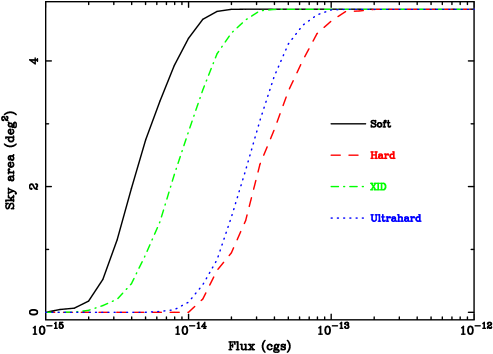
Figure 1: Sky area as a function of flux for different bands

4 The log$N$-log$S$

We have first studied the sky density of the detected sources as a function of flux (known as the log$N$-log$S$) in the soft, hard, XID and ultra-hard bands.

4.1 Sky areas

The sky area over which we are sensitive to a given flux is easy to calculate from the sensitivity maps. In principle, we just need to sum the sky area over which the sensitivity maps have values below the desired flux. However, the conversion between flux and count rate depends on the assumed spectral shape. In each band $i$, we have calculated the sky areas at each flux for each assumed spectral slope $\Omega_{i}(S,\Gamma)$ with the following procedure: in each field, we have converted $S$ to count rate using $\Gamma$ and the response matrices, and summed the area over which the sensitivity map is below that count rate. The total sky area is the sum of the areas found for each field.

The sky area in each band for each source $j$ is then $\Omega_{j,i}=\Omega_{i}(S_{j,i},\Gamma_{j,i})$, where the source’s flux $S_{j,i}$ and spectral slope $\Gamma_{j,i}$ are described in Section 3.

Sky areas independent of any assumed spectrum can also be obtained by weighting $\Omega_{i}(S,\Gamma)$ with the number of detected sources in each $(S,\Gamma)$ bin. We will call these spectrally averaged sky areas $\Omega_{i}(S)$. They are shown in Fig. 1. The maximum value of all curves is 4.8 deg², which is the geometric area covered by our survey, taking into account the excluded areas.

We have also obtained spectrally averaged sky areas for each field $\Omega_{i,k}(S)$ ($k=1\ldots$number of fields) from the sensitivity maps for each field $k$ in each band $i$, using $S(\Gamma)$ for that field, and weighting with the number of sources in the total sample with the corresponding $S,\Gamma$, assuming implicitly that all fields have the same $S(\Gamma)$ distribution.

4.2 Data from other surveys

Our survey consists of XMM-Newton exposures with a typical exposure time of about 15 ks, and it is hence a medium survey. Shallower wider area surveys are required to obtain significant numbers of bright sources, while deeper pencil-beam surveys will probe fainter fluxes. We have combined our survey with both shallower and deeper surveys to obtain a wide coverage in flux ($\sim$2-4 orders of magnitude):

• BSS: Della Ceca et al. (DellaCeca04 (2004)) have constructed a bright sample of XMM-Newton sources down to a flux of $7\times 10^{-14}$ cgs in the XID band, with a uniform coverage of 28.1 deg² above that flux. This sample is ideally complementary to our XID, being both wider and shallower, and selected exactly in the same band with the same observatory (but with a different detector: MOS2 instead of pn). We have used a total of 389 sources from that survey, including all sources identified as stars, which have been excluded from the log$N$-log$S$ analysis of Della Ceca et al. (DellaCeca04 (2004))

• HBS: In the same paper, Della Ceca et al. (DellaCeca04 (2004)) also define a sample of sources detected in the ultra-hard band, down to the same flux limit, and with a uniform coverage of 25.17 deg², again both shallower and wider than ours and with the same observatory. Results from a subsample are presented by Caccianiga et al. (HBS28 (2004)). The source counts are also discussed by Della Ceca et al. (DellaCeca04 (2004)) and compared to previous results from BeppoSAX. We have used a total of 65 sources from this survey

• CDF: The deepest survey in the soft and hard bands so far is the Chandra Deep Field North (CDF-N) Bauer et al. (Bauer04 (2004)), obtained from a total exposure of 2 Ms in a location in the Northern hemisphere. In a complementary effort in the South, the Chandra Deep Field South (Giacconi et al. Giacconi01 (2001), Rosati et al. Rosati02 (2002)) gathered a total of 1 Ms. Source counts from both samples have been discussed in Bauer et al. (Bauer04 (2004)). There are a total of 442 soft and 313 hard sources in the CDF-N, and 282 soft and 186 hard sources in the CDF-S. Recent internal Chandra calibrations have increased the estimate of the ACIS effective area above 2 keV. We have used the applications on the Chandra calibration database to compare data from Cycles 8 and 5: above 2 keV the ratio between the effective areas is reasonably flat, and well approximated by a constant increase factor of about 12%. The increase in the 2-8 keV fluxes is unlikely to be due to the increasing contamination from the optical blocking filter, since the latter only manifests itself below  1 keV. Therefore, all CDF-N and CDF-S hard fluxes (and their corresponding errors) have been decreased by this factor. Furthermore, when comparing the sky areas calculated individually for each source with those calculated interpolating from the sky area of the full survey, the faintest soft sources in both CDF surveys showed large (up to several orders of magnitude) discrepancies. Since our maximum likelihood log$N$-log$S$ fit method requires the use of a model for the sky area of the full survey (see Section 4.5), we have not used soft sources fainter than 3 and 7$\times 10^{-17}$ cgs in the CDF-N and CDF-S respectively in the log$N$-log$S$ fit.

• AMSS: The ASCA Medium Sensitivity Survey (Ueda et al. Ueda05 (2005)) is one of the largest high Galactic latitude broad-band X-ray surveys to date, including 606 sources over 278 deg² with hard band fluxes between $\sim 10^{-13}$ and $\sim 10^{-11}$ cgs.

The average sky area as a function of flux for different bands for the CDF and AMSS are shown in Bauer et al. (Bauer04 (2004)) and Ueda et al. (Ueda05 (2005)), respectively. We obtained them from the respective first authors, and we have used them for the Maximum Likelihood fit (see Section 4.5). The Chandra re-calibration has also been applied to the CDF effective area fluxes.

Table 5: Maximum likelihood fit results to the log$N$-log$S$ in different bands and using different samples: the first column is the band used, the second is the power-law slope above the flux break, the third is the slope below that break, the fourth is the flux break, the fifth is the normalisation, the last six columns indicate the number of sources from each sample used in the fit.

					$N_{\rm used}/N_{\rm tot}$
Band	$\Gamma_{u}$	$\Gamma_{d}$	$S_{b}$	$K$	AXIS	BSS	HBS	CDF-N	CDF-S	AMSS
			($10^{-14}$ cgs)	(deg-2)
softg	2.40${}^{+0.06}_{-0.07}$	1.74${}^{+0.06}_{-0.07}$	1.15${}^{+0.18}_{-0.19}$	120.0${}^{+22}_{-18}$	1267/1267
soft	2.39${}^{+0.06}_{-0.06}$	1.69${}^{+0.07}_{-0.06}$	1.15${}^{+0.16}_{-0.13}$	123.4${}^{+18.8}_{-17.1}$	1267/1267
softf	2.38${}^{+0.14}_{-0.09}$	1.56${}^{+0.01}_{-0.01}$	1.02${}^{+0.14}_{-0.17}$	141.4${}^{+42.1}_{-7.3}$	1267/1267			429/442a	269/282b
hardg	2.74${}^{+0.08}_{-0.07}$	-	1.00	735 ${}^{+92}_{-76}$	348/397c
hard	2.72${}^{+0.07}_{-0.08}$	-	1.00	684.4${}^{+74.1}_{-84.0}$	348/397c
hard	2.03${}^{+0.12}_{-0.11}$	1.00${}^{+0.11}_{-0.12}$	0.30${}^{+0.07}_{-0.05}$	1086.6${}^{+134.3}_{-146.5}$				313/313
hard	2.51${}^{+0.50}_{-0.28}$	0.89${}^{+0.12}_{-0.12}$	0.72${}^{+0.11}_{-0.10}$	743.7${}^{+109.6}_{-105.6}$					186/186
hard	2.12${}^{+0.13}_{-0.01}$	1.10${}^{+0.01}_{-0.01}$	0.44${}^{+0.04}_{-0.01}$	799.1${}^{+226.8}_{-8.4}$				313/313	186/186
hard	2.66${}^{+0.08}_{-0.05}$	1.20${}^{+0.01}_{-0.01}$	1.00${}^{+0.08}_{-0.01}$	611.5${}^{+49.1}_{-34.3}$	397/397			313/313	186/186
hard	2.58${}^{+0.02}_{-0.02}$	-	1.00	606.5${}^{+46.8}_{-46.3}$	348/397c					606/606
hard	2.53${}^{+0.25}_{-0.18}$	1.18${}^{+0.14}_{-0.08}$	0.92${}^{+0.66}_{-0.19}$	607.8${}^{+366.4}_{-208.1}$				313/313	186/186	606/606
hardf	2.58${}^{+0.17}_{-0.02}$	1.30${}^{+0.01}_{-0.01}$	1.17${}^{+0.01}_{-0.05}$	485.3${}^{+10.1}_{-24.3}$	397/397			313/313	186/186	606/606
XIDg	2.39${}^{+0.05}_{-0.20}$	1.37${}^{+0.09}_{-0.32}$	1.08${}^{+0.07}_{-0.48}$	265 ${}^{+214}_{-19}$	1359/1359
XID	2.46${}^{+0.11}_{-0.07}$	1.29${}^{+0.09}_{-0.18}$	1.45${}^{+0.16}_{-0.26}$	212.2${}^{+47.4}_{-22.8}$	1359/1359
XIDf	2.54${}^{+0.03}_{-0.04}$	1.35${}^{+0.06}_{-0.25}$	1.64${}^{+0.13}_{-0.28}$	193.0${}^{+33.1}_{-15.8}$	1359/1359	389/389
ultra-hardg	2.63${}^{+0.15}_{-0.15}$	-	1.00	102 ${}^{+23}_{-20}$	84/89d
ultra-hard	2.59${}^{+0.09}_{-0.05}$	-	1.00	95.0${}^{+11.1}_{-12.8}$	84/89d
ultra-hardf	2.62${}^{+0.10}_{-0.10}$	-	1.00	102.2${}^{+20.0}_{-21.1}$	84/89d		58/65e

• $S_{\rm min,CDF-N}=3\times 10^{-17}$ cgs

• $S_{\rm min,CDF-S}=6\times 10^{-17}$ cgs

• $S_{\rm min,AXIS}=1.5\times 10^{-14}$ cgs

• $S_{\rm min,AXIS}=10^{-14}$ cgs

• $S_{\rm max,HBS}=2.5\times 10^{-13}$ cgs

• Best fit used for contribution to XRB, and in Figs. 2 and 3.

• Using fixed photon indices of 1.8 in the soft and XID bands, and 1.7 in the hard and ultra-hard bands.

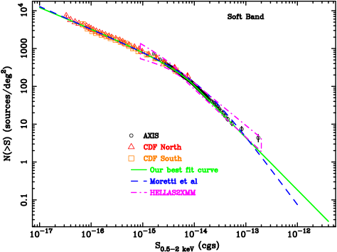
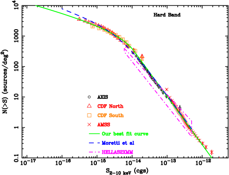
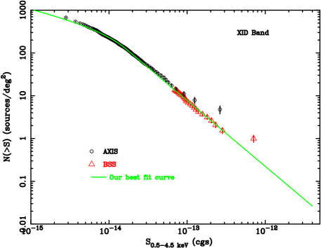
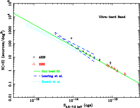
Figure 2: Integral log$N$-log$S$ in different bands, along with our best fits and some previous results

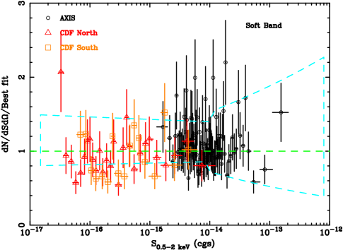
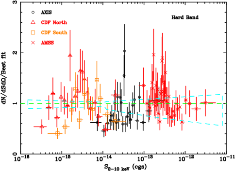
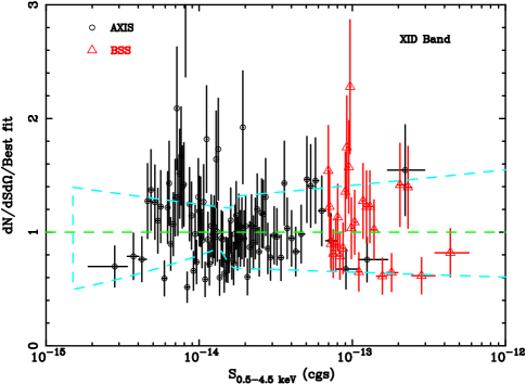
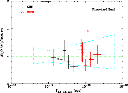
Figure 3: Ratio between the binned differential log$N$-log$S$ and the best fit model in different bands. The 1-$\sigma$ uncertainty interval on the log$N$-log$S$ is also shown as bow-tie-shaped dashed lines above and below unity.

4.3 Construction of the binned log$N$-log$S$

The binned differential log$N$-log$S$ (number of sources per unit flux and unit sky area at a given flux $S$: $dN/dSd\Omega$) have been constructed summing the inverse of the $\Omega_{j,i}$ for the sources in each flux bin, and dividing that number by the width of the bin. The errors are calculated dividing the $dN/dSd\Omega$ by the square root of the sources in each bin. Since we have chosen to have a minimum number of sources per bin (see below), their widths are all in principle different, determined by the flux of the first source in the bin and the flux of the first source in the next bin going up in flux. With this definition, the width of the last bin was left undefined. Since we have a large number of sources, we have dropped the brightest source in each sample (only when dealing with binned log$N$-log$S$), defining the upper limit in the last bin to be the flux of this brightest source.

The integral log$N$-log$S$ (number of sources per unit sky area with fluxes higher than $S$: $N(>S)$) from our sample and other samples are shown in Fig. 2. We have chosen to plot the integral log$N$-log$S$ in bins containing 15 sources each (except the last one, which can contain up to 29 sources), to avoid apparent features due to fluctuations of a few sources, specially at the brighter ends of each sample, were the number of sources is low. We have simply added the inverse of the sky areas for each source $\Omega_{j,i}$, for all sources with fluxes above the lower limit of each bin. The error bars are calculated dividing the $N(>S)$ by the square root of the total number of sources with flux equal or greater than the lower limit of the bin.

Sources just below the faint flux limit of a survey could experience statistical fluctuations of their fluxes, promoting them into the survey, the fainter sources just above that limit could drop from the survey for the same reason, but since fainter sources are much more abundant (because the source counts are steep), the net effect is to increase artificially the observed source counts close to the fainter survey limits. This is known as the Eddington bias (Eddington Eddington13 (1913)), and sometimes causes a re-steepening of the log$N$-log$S$ at the faintest fluxes, as observed in the AXIS ultra-hard source counts, for example.

4.4 log$N$-log$S$ model

Previous X-ray source count results (e.g. Bauer et al. Bauer04 (2004), Ueda et al. Ueda03 (2003), Moretti et al. Moretti03 (2003), Baldi et al. Baldi02 (2002), Hasinger et al. Hasinger98 (1998), Cagnoni, Della Ceca & Maccacaro Cagnoni98 (1998)) have shown that the log$N$-log$S$ is well approximated by a steep power law at bright fluxes, flattening at lower fluxes. We have hence adopted the following model for the differential log$N$-log$S$:

$${dN\over dSd\Omega}(S)=\left\{\begin{array}[]{ll}{K\over S_{b}}\left({S\over S_{b}}\right)^{-\Gamma_{d}}&,S\leq S_{b}\\ {K\over S_{b}}\left({S\over S_{b}}\right)^{-\Gamma_{u}}&,S>S_{b}\\ \end{array}\right\}$$

The above model has four independent parameters: the break flux $S_{b}$, the normalisation $K$, the slope at high fluxes $\Gamma_{u}$, and the slope at low fluxes $\Gamma_{d}$. If the change in the slope of the log$N$-log$S$ is not significant, we fixed $S_{b}\equiv 10^{-14}$ cgs and $\Gamma_{u}=\Gamma_{d}$, leaving only two independent variables: $K$ and $\Gamma_{u}$.

The integral log$N$-log$S$is therefore:

$$N(>S)=\int_{S}^{\infty}dS{dN\over dSd\Omega}(S)$$

Finally, assuming a given log$N$-log$S$, the number of sources with fluxes between $S_{\rm min}$ and $S_{\rm max}$ is

$$N(S_{\rm min}\leq S\leq S_{\rm max})=\int_{S_{\rm min}}^{S_{\rm max}}dS{dN\over dSd\Omega}(S)\Omega(S)$$

This number is the total expected number of sources in our survey $\lambda$ with fluxes in band $i$ in that interval if $\Omega(S)=\Omega_{i}(S)$ defined above, or it can be $\lambda_{k}$ the expected number of sources in that flux interval and band in a given field $k$ if $\Omega(S)=\Omega_{i,k}(S)$.

The contribution to the intensity of the XRB from the interval $(S_{\rm min},S_{\rm max})$ is

$$I(S_{\rm min}\leq S\leq S_{\rm max})=\int_{S_{\rm min}}^{S_{\rm max}}dS\,S{dN\over dSd\Omega}(S)$$ (1)

4.5 Maximum likelihood fit method and results

We have fitted the log$N$-log$S$ using a Maximum Likelihood method which takes into account the uncertainties on the fluxes of the sources, as well as the changing shape of the sky areas with flux.

Specifically, we have minimised the following expression:

$$L_{\rm tot}=\sum_{\rm sample}L_{\rm sample}$$

where $L_{\rm sample}$ is given by

$$L_{\rm sample}=-2\sum_{j=1}^{N}\log(P(S_{j}))-2\log(P_{\lambda}(N))$$ (2)

where the sum is over all the $N$ sources in the corresponding sample, and $P(S_{j})$ is the probability of finding a source of flux $S_{j}$ in that sample (see below). The second term is $P_{\lambda}(N)=e^{-\lambda}\lambda^{N}/N!$ the Poisson probability of finding $N$ sources in that sample when the expected number is $\lambda$ (see Section 4.4).

We have defined $P(S_{j})$ as

$$P(S_{j})={{\int_{S^{\prime}_{\rm min}}^{S^{\prime}_{\rm max}}dS{dN\over dSd\Omega}(S)\Omega(S){\exp\left(-(S_{j}-S)^{2}\over 2\sigma_{j}^{2}\right)\over\sqrt{2\pi}\sigma_{j}}}\over\lambda}$$

This expression takes into account both the variation of the sky area with flux (through $\Omega(S)$), and the uncertainty in the flux of the source $\sigma_{j}$ (Page et al. Page00 (2000)), through the last exponential term in the numerator, in which we have assumed a Gaussian distribution of the fluxes around the measured value. To speed up the numerical calculation of the integral in the numerator above, we have defined $S^{\prime}_{\rm min}={\rm max}(S_{j}-4\sigma_{j},S_{\rm min})$ and $S^{\prime}_{\rm max}={\rm min}(S_{j}+4\sigma_{j},S_{\rm max})$, since the tails of the Gaussian distribution decrease very quickly. The normalisation of the log$N$-log$S$ ($K$) appears both in the numerator and the denominator of $P(S_{j})$ and it is unconstrained. This is why we have introduced the second term in Eq. 2.

The 1-$\sigma$ uncertainties in the log$N$-log$S$ parameters are estimated from the range of each parameter around the minimum which makes $\Delta L_{\rm tot}=1$. For each parameter, this is done by fixing the parameter of interest to a value close to the best fit value, and varying the rest of the parameters until a new minimum for the likelihood is found, this is repeated for several values of the parameter until this new minimum equals $L_{\rm tot,min}+1$.

The results of the Maximum Likelihood fits to various (single and combined) samples and bands are given in Table 5. Except when stated otherwise, the flux interval used in the fit is $S_{\rm min}=10^{-17}$ cgs and $S_{\rm max}=10^{-12}$ cgs. These numbers have been chosen to span the observed fluxes of the sources. The final results are not very dependent on them, since the sky area falls very quickly at low fluxes, and the sky density of bright sources is very small. The initial values for the numerical search for the best fit have been obtained from a $\chi^{2}$ fit to the total binned differential log$N$-log$S$. The best overall fits are marked in the first column of Table 5 and also shown in Fig. 2.

The first two rows in Table 5 for each band allow comparing the results of the fit to the AXIS sources using a fixed spectral slope to calculate fluxes and sky areas ($\Gamma=1.8$ in the soft and XID bands, $\Gamma=1.7$ in the hard and ultra-hard bands, first row), to the results using the best fit spectral slope for each source (second row). The results are mutually compatible in all bands, but the error bars are noticeably larger in the XID and ultra-hard band when using a fixed spectral slope. Since by fitting the spectra of the sources we are “forcing” them to have a power law spectral shape, the uncertainties in the fitted fluxes are smaller than those in the fluxes with fixed spectral slopes. This might explain at least in part the smaller uncertainties in the log$N$-log$S$ fitted parameters in the latter case. In what follows, we have hence used the slopes from spectral fits to calculate fluxes from count rates for all the AXIS sources, since this approach seems to produce smaller uncertainties in the fitted parameters.

There is general agreement between data and model fits, but it is difficult to quantify this statement, since, unlike the $\chi^{2}$ statistic, the absolute value of $L_{\rm tot}$ is not an indicator of the goodness of the fit. Each panel in Fig. 2 covers several orders of magnitude, and hence a detailed visual comparison is also difficult. We have therefore plotted in Fig. 3 the ratio between the binned differential log$N$-log$S$ and the best fit model. Systematic deviations from unity in those plots would reveal differences between the data and the best fit model. In that Figure we also show the 1-$\sigma$ uncertainty interval on the best fit, estimated in a conservative way: for each flux, we have calculated the differential log$N$-log$S$ in the 16 corners of the hypercube defined by the 1-$\sigma$ uncertainty intervals in the best fit log$N$-log$S$ parameters, and taken the maximum and minimum values.

As expected, the relative agreement of the AXIS and BSS/HBS source counts is quite good, merging with each other well, and following the same log$N$-log$S$ shape. This confirms the good relative calibration of the two EPIC cameras on board XMM-Newton (pn for AXIS and MOS2 for BSS/HBS). The XMM-COSMOS log$N$-log$S$ results (Cappelluti et al. Cappelluti07 (2007)), are also consistent with ours within 1 to 2-$\sigma$ in the soft and hard bands, but the uncertainties in our best fit parameters are smaller, probably due to our much higher number of sources and wider flux coverage in those bands.

The agreement with the CDF samples is very good. In the soft band, our joint AXIS-CDF fit is in excellent agreement with the CDF results of Bauer et al. (Bauer04 (2004)) ($\Gamma_{d}=1.55\pm 0.03$), as expected since virtually all sources at low fluxes are the same in both samples. Our AXIS-only fit prefers a steeper slope below the break, but still compatible with the joint AXIS-CDF fit at $<2\sigma$. The agreement with Moretti et al. (Moretti03 (2003)) is very good below the break ($\Gamma_{d}=1.60^{+0.02}_{-0.03}$, hereafter we have translated all integral log$N$-log$S$ slopes to our differential slopes), but their break happens at higher fluxes ($S_{b}=(1.5\pm 0.3)\times 10^{-14}$ cgs), resulting in a steeper slope at high fluxes ($\Gamma_{u}=2.82^{+0.07}_{-0.09}$). Our results are fully compatible with those of the HELLAS2XMM (Baldi et al. Baldi02 (2002)) sample at their low flux end, but our source counts are systematically at their lower envelope above the break.

In the hard band, the CDF, AXIS and AMSS log$N$-log$S$ match well in their overlapping regions. However, the ratio in the top-right panel of Fig. 3 is rather wiggly and shows clear differences in detail. The AXIS data are mostly below the model, perhaps because (see Section 2.4) the high fraction of sources excluded for being fainter than the sensitivity map, and the relatively lower value of the sensitivity map with respect to the Poisson count rate (which would in turn increase the effective area). There are two “bumps” with the data systematically above the model at about $3\times 10^{-15}$ and $3\times 10^{-13}$ cgs (although in this last one the discrepancy is well inside the uncertainties on the log$N$-log$S$ fit). These bumps probably arise from fitting a broken power-law with a sharp break to the log$N$-log$S$, which is really a smooth distribution coming from the superposition of different populations at different redshifts. This is compounded by possible calibration uncertainties: the hard band calibration of Chandra has changed by 12% in the last 3 years (see Section 4.2).

A break at $3\times 10^{-15}$ cgs is actually present in the joint fit to the CDF-N and CDF-S hard (all-CDF) samples (see Table 5), with the low flux slope compatible with the value from Bauer et al. Bauer04 (2004) ($\Gamma_{d}=1.56\pm 0.14$) within about 1-$\sigma$, and the high flux slope flatter than in the global fit. The low flux slopes for the two single CDF samples are much flatter than and incompatible with any previously reported values ($\sim 1$). We believe that the change in the slope of the source counts between AXIS and the CDF forces the global break flux to the overlapping fluxes between those samples ($\sim 10^{-14}$ cgs), and hence the fit below this flux somehow averages the two slopes present in the CDF, forming a bump around the CDF break, rising and dropping above and below this flux, respectively. The overall behaviour of the log$N$-log$S$ can be obtained by a fit to the CDF and AMSS data alone, and, despite the lower AXIS source counts, the best fit values between the CDF+AMSS and the CDF+AMSS+AXIS are mutually compatible within $<$1-$\sigma$, the main effect being pushing the break flux to higher fluxes and steepening the low flux slope. Additionally, the uncertainties in all parameters are significantly reduced by the inclusion of the AXIS data, by factors between about 2 and 20.

The best fit curve by Moretti et al. (Moretti03 (2003)) is again very similar to our all-sample fit at the highest ($\Gamma_{u}=2.57^{+0.10}_{-0.08}$) and lowest fluxes ($\Gamma_{d}=1.44^{+0.12}_{-0.13}$), where it is however above the CDF data (perhaps because of the change in the hard band calibration of Chandra). Their transition flux occurs at lower fluxes ($S_{b}=(4.5^{+3.7}_{-1.7})\times 10^{-15}$ cgs), compatible with the CDF-N and all-CDF fits, perhaps because their functional form is smoother than a broken power-law and cannot accommodate the relatively strong break between the AMSS/AXIS steep slope and the CDF. The HELLAS2XMM confidence interval overlaps with ours, but has a flatter slope, and falls clearly below both the AXIS and the CDF points below about $2\times 10^{-14}$  cgs, perhaps suggesting incompleteness at their lower fluxes.

Our fit to the joint AXIS-BSS source counts in the XID band looks visually quite good, passing through the middle of the AXIS and BSS data points (see Fig. 2). The XID band source counts from the BSS (Della Ceca et al. DellaCeca04 (2004)) require a steeper slope ($\Gamma_{u}=2.80\pm 0.11$) than both our AXIS-only and AXIS+BSS fits. The origin of this apparent discrepancy is probably that we have used all the selected sources in both samples, while they have excluded the stars, which contribute more at higher fluxes, and hence would produce a steeper source count distribution, as observed.

The AXIS-only ultra-hard source counts merge smoothly with the HBS, if we ignore our higher flux point (which could be affected by the exclusion of the bright targets in our survey). We have not used AXIS sources with fluxes below $10^{-14}$ cgs in the fit because the log$N$-log$S$ steepens suddenly at those fluxes, perhaps because the Eddington bias is most important in this band where the number of sources is smallest, and/or because of the contribution from spurious sources. The best fit values including these lowest flux sources are very similar to the ones excluding them, but the errors on the values are much larger. Since the ML fit is dominated by the bulk of the sources, rather than by a few discrepant points, and given the low number of sources, the AXIS-only and AXIS+HBS source counts are very similar and mutually compatible. They are also compatible as well with the HBS-only value ($\Gamma_{u}=2.64^{+0.25}_{-0.23}$), despite the fact that this log$N$-log$S$ again only includes the extragalactic sources. The reason why the discrepancy is almost unnoticeable in the ultra-hard band is probably because the stars contribute negligibly to the high Galactic latitude source counts in this energy band.

We have compared our ultra-hard (4.5-7.5 keV) source counts to some previous results in the 5-10 keV band, assuming a photon index of 1.7 for the flux conversion between these bands. Our source count slope is slightly steeper than in Baldi et al. (Baldi02 (2002), $\Gamma_{u}=2.54^{+0.25}_{-0.19}$) and flatter than in Loaring et al. (Loaring05 (2005), $\Gamma_{u}=2.80^{+0.67}_{-0.55}$), but well within the 1-$\sigma$ limits in both cases. The source counts from Rosati et al. (Rosati02 (2002), $\Gamma_{u}=2.35\pm 0.15$) are much flatter, but still compatible with ours within less than 2-$\sigma$. They also find an indication of a break in the source counts at a 5-10 keV flux of $4\times 10^{-15}$ cgs (or about $3\times 10^{-15}$ cgs in the ultra-hard band). Since they also reach fainter fluxes ($S_{\rm ultra-hard}\sim 1.6\times 10^{-15}$ cgs), their flatter source count slope probably arises from a combination of an Euclidean slope at brighter fluxes and an even flatter slope at their faintest fluxes. Our absolute source counts agree well with both Loaring et al. (Loaring05 (2005)) and Rosati et al. (Rosati02 (2002)) at their brightest flux limits, and this agreement is maintained for our best fit log$N$-log$S$ over the whole flux interval in the former case, while the latter is clearly flatter and below our best fit, indicating a flattening of the ultra-hard source counts below our flux limit as discussed above. The XMM-COSMOS ultra-hard number counts coincide with ours at the lowest fluxes ($\sim 10^{-14}$ cgs), but they are above ours at higher fluxes, although within their relatively large error bars.

Table 6: Intensity in different bands from different origins and flux intervals. The first column indicates the band, the second gives the origin of the intensity, the third and fourth columns list the flux interval, the fifth column total intensity from that interval, the sixth column shows the fraction of the XRB intensity contributed by sources in that interval.

Band	Origin	$S_{\rm min}$	$S_{\rm max}$	$I(S_{\rm min}\leq S\leq S_{\rm max})$	$f_{\rm XRB}$
		(cgs)	(cgs)	($10^{-12}$ cgs deg-2)
soft	Best fit AXIS+CDF log$N$-log$S$	0	$3\times 10^{-17}$	0.25	0.03
soft	Best fit AXIS+CDF log$N$-log$S$	$3\times 10^{-17}$	$2\times 10^{-13}$	5.60	0.75
soft	Best fit AXIS+CDF log$N$-log$S$	$3\times 10^{-17}$	$10^{-11}$	6.54	0.87
soft	RBS sourcesa	$10^{-11}$		0.20	0.03
soft	Total resolved	$3\times 10^{-17}$		6.55e	0.87
soft	XRBb			$7.5\pm 0.4$
hard	Best fit AXIS+CDF+AMSS log$N$-log$S$	0	$3\times 10^{-16}$	0.62	0.03
hard	Best fit AXIS+CDF+AMSS log$N$-log$S$	$3\times 10^{-16}$	$1\times 10^{-11}$	17.08	0.85
hard	Best fit AXIS+CDF+AMSS log$N$-log$S$	$3\times 10^{-16}$	$3.1\times 10^{-11}$	17.18	0.85
hard	HEAO-1 A2 sourcesc	$3.1\times 10^{-11}$		0.43	0.02
hard	Total resolved	$3\times 10^{-16}$		17.25e	0.85
hard	XRBb			$20.2\pm 1.1$
XID	Best fit AXIS+BSS log$N$-log$S$	$3\times 10^{-15}$	$10^{-12}$	8.48	0.56
XID	Best fit AXIS+BSS log$N$-log$S$	$3\times 10^{-15}$	$2.38\times 10^{-11}$	9.00	0.59
XID	Bright sourcesd	$2.38\times 10^{-11}$		0.39	0.02
XID	Total resolved	$3\times 10^{-15}$		9.20e	0.60
XID	XRBd			$15.3\pm 0.6$
ultra-hard	Best fit AXIS+HBS log$N$-log$S$	$9\times 10^{-15}$	$2\times 10^{-13}$	1.50	0.21
ultra-hard	Best fit AXIS+HBS log$N$-log$S$	$9\times 10^{-15}$	$1.05\times 10^{-11}$	1.74	0.24
ultra-hard	Bright sourcesd	$1.05\times 10^{-11}$		0.15	0.02
ultra-hard	Total resolved	$9\times 10^{-15}$		1.79e	0.25
ultra-hard	XRBd			$7.2\pm 0.4$

• Schwope et al. (Schwope00 (2000))

• Moretti et al. (Moretti03 (2003))

• Piccinotti et al. (Piccinotti82 (1982))

• See text

• After subtracting the stellar contribution (see Section 5.1)

5 Contribution to the X-ray background

Using the best fit parameters from Table 5, we can estimate the intensity contributed by sources in different flux intervals (Eq. 1). In order to compare the total intensity contributed by resolved sources with the total XRB intensity, we need to estimate the intensity from sources brighter than our survey limit (see Section 5.1), and to adopt a total XRB intensity (see Section 5.2).

5.1 Intensity from bright sources and stars

The contribution from bright sources is straightforward to obtain for the “traditional” soft and hard bands. For the soft band we have followed the same method as Moretti et al. (Moretti03 (2003)) summing the fluxes of the sources in the Rosat Bright Survey (RBS, Schwope et al. Schwope00 (2000)) with soft flux higher than $10^{-11}$ cgs, and dividing by the area covered by the RBS. For the hard band we have used the sources in the HEAO-1 A2 survey (Piccinotti et al. Piccinotti82 (1982)), which is complete down to $3.1\times 10^{-11}$ cgs. We have estimated the contribution of bright sources for the ultra-hard band from the hard band values, converting both the flux limit and the intensity to the ultra-hard band using a power-law with slope $\Gamma=1.7$. The XID band strides the hard and soft bands and it is necessary to combine measurements taken in different bands and with different instruments. We have estimated the 2-4.5 keV flux limit and intensity from the hard band values using again $\Gamma=1.7$, and added both of them to the soft band values.

Since the estimates of the XRB intensity discussed below are for the extragalactic XRB, we need to estimate the contribution from Galactic stars down to our fainter flux limits, in order to subtract it from our estimated source intensities and get the resolved fraction of the extragalactic XRB. We take the estimates of Bauer et al. (Bauer04 (2004)) from the fractions in their Table 2 and their assumed total XRB intensities: $0.19^{+0.05}_{-0.04}\times 10^{-12}$ and $0.36^{+0.34}_{-0.19}\times 10^{-12}$ cgs deg^-2 from stars in the soft and hard bands respectively. Since most of the contribution from stars comes from high fluxes (Bauer et al. Bauer04 (2004)), and the stars at those fluxes have mainly low temperature thermal spectra (Della Ceca et al. DellaCeca04 (2004)), we have estimated the stellar contribution in the XID band from the soft band contribution assuming a 0.5 MK mekal model under xspec, obtaining an XID-to-soft flux ratio of 1. Our estimate of the XID band intensity from Galactic stars is thus $0.19^{+0.05}_{-0.04}\times 10^{-12}$ cgs deg^-2. This is a conservative estimate, since the source counts in the XID band are about one order of magnitude shallower than in the soft band. Using that same spectral model, the stellar contribution in the 1-2 keV band is $(0.036\pm 0.010)\times 10^{-12}$ cgs deg^-2. Given the even higher flux limit in the ultra-hard band, and the strong dependence of the thermal spectrum with energy, we have instead estimated the stellar contribution to the ultra-hard band intensity by summing the fluxes of the two sources identified as stars in the HBS, and dividing it by the sky coverage of that survey, obtaining $(0.099\pm 0.005)\times 10^{-12}$ cgs deg^-2. No sources have been identified as stars among the 60 identified XMS deeper ultra-hard survey sources (Barcons et al. Barcons06b (2007)), and all of the 10 remaining unidentified objects in that sample are extended. This lower fraction of stellar identifications of X-ray sources as the flux decreases and the band hardens, is consistent with the average soft thermal X-ray spectra of stars and their flat source counts (Bauer et al. Bauer04 (2004)).

Figure 4: Relative contribution to the “total” intensity from equally spaced logarithmic flux intervals, using the best fit models in each band (see text): soft (solid line), hard (dashed), XID (dot-dashed) and ultra-hard (dotted).

5.2 Total X-ray background intensity

The total extragalactic XRB intensity measured with different instruments produces different results (Barcons et al. Barcons00 (2000)), and not all the differences are attributable to cosmic variance. Moretti et al. (Moretti03 (2003)) have averaged several measurements available in the literature in the 1-2 keV and hard bands, obtaining $4.54\pm 0.21$ and $20.2\pm 1.1$ (in units of $10^{-12}$ cgs deg^-2), respectively. We have used those values to estimate the XRB intensity in our bands assuming a power-law with $\Gamma=1.4$, which is an adequate model for the extragalactic XRB spectrum above 2 keV (Lumb et al. Lumb02 (2002)). The extrapolation of the value of Moretti et al. (Moretti03 (2003)) in the hard band to the 1-2 keV band using that spectral shape produces a value similar to the one obtained directly by them in that band, this justifies extrapolating again the same spectral shape down to 0.5 keV, although the shape of the XRB is poorly known below 1 keV. The results are given in Table 6.

Our adopted hard band XRB intensity (from Moretti et al.) is in agreement with the estimate from Lumb et al. (Lumb02 (2002), $21.5\pm 2.6$ in the above units), and compatible with the result of De Luca & Molendi (DeLuca04 (2004), $22.4\pm 1.6$) within about 1-$\sigma$. Extrapolating those intensities to the soft band using $\Gamma=1.4$ we obtain $7.46\pm 0.09$ and $7.78\pm 0.06$, respectively, again fully compatible with our adopted value of $7.5\pm 0.4$.

Recently, Hickox & Markevitch (HM06 (2006), henceforth HM06) have re-estimated the total XRB intensity in the 1-2 keV and 2-8 keV bands, using Chandra CDF data, and contributions from brighter sources. They have analysed thoroughly the non-cosmic background in Chandra, and isolated unresolved components of the XRB in those bands, which are only about $\sim$20% and $\sim$4% of the non-cosmic background contributions in those bands, respectively. The origin of this unresolved components is unknown. One possibility is stray light from sources outside the field of view. The HM06 total XRB intensity estimates in those bands are obtained by summing to these unresolved components the contributions from the resolved sources in the CDF data, and from brighter sources using the log$N$-log$S$ of Vikhlinin et al. (Vikhlinin95a (1995)), with different spectral slopes at different fluxes. Their 1-2 keV intensity is $4.6\pm 0.3$ (in the above units), very similar to our adopted value. With their estimates of the total XRB intensity, the total resolved fractions of the XRB are only $77\pm 3$% and $80\pm 8$% in the 1-2 keV and 2-8 keV bands, respectively, lower than previous estimates, in particular in the softer band. We will discuss the origin of these differences in Section 5.4

5.3 Contribution of different flux intervals to the X-ray background

X-ray intensities are shown in Table 6 for the observed flux intervals in the samples used here, and for flux intervals with higher maximum fluxes, chosen to “join” the observed intervals with the contribution from bright sources, which are also given in that table, as well as the XRB intensities from Moretti et al. (Moretti03 (2003)).

We have plotted in Fig. 4 the relative contribution of two flux intervals per decade to the total XRB intensity for the four default bands, assuming our best fit log$N$-log$S$. It is clear that the maximum contribution comes from fluxes around the break flux $\sim 10^{-14}$ cgs. The contribution from the bins in one decade around that value are close to 50% of the total in the soft and hard bands. In the ultra-hard band we do not reach deep enough to detect the break. From the 5-10 keV band source counts of Hasinger et al. (Hasinger01 (2001)) and Rosati et al. (Rosati02 (2002)), there could be a break just below $\sim 10^{-14}$ cgs.

The extrapolation the soft and hard log$N$-log$S$ to zero flux using our best fit model (see Table 6) does not saturate the XRB intensity (although in the soft band total XRB intensity is within the intensities spanned by the uncertainties in the best fit log$N$-log$S$ parameters). This suggests that the possibility of a new dominant population at lower fluxes is still open, mainly in the hard band. Under the assumption that the fraction of truly diffuse XRB is negligible (and the fluctuation analysis of Miyaji & Griffiths Miyaji02 (2002) shows that the source counts continue growing in the soft band down to at least $7\times 10^{-18}$ cgs), it is possible to estimate the minimum source counts slope necessary to just saturate the XRB at zero flux, if the source counts steepened just below the minimum flux studied here. Those slopes are 1.85 and 1.84 in the soft and hard bands, respectively. Comparing these values to the observed slopes of the separate AGN and galaxy source counts in the CDF (Bauer et al. Bauer04 (2004)), only the absorbed AGN (slope $\sim 1.62$, versus 1.2-1.5 for the rest of the AGN estimates) come close to be able to saturate the soft XRB, while galaxies can do it with just about any estimate for their source counts slope (2.1-2.7), if it keeps growing at the same rate below the resolved fluxes. The situation in the hard band is again the same, with the absorbed AGN (source counts slope 1.95, versus 1.4-1.5) being the only AGN population able to contribute the rest of the unresolved intensity, while the galaxy source counts estimates (slope 3-3.5) could easily fulfil this role. A similar conclusion is reached if a higher intensity for the XRB is adopted (HM06), since this would steepen the faint source counts slope required to saturate the XRB.

Even if the source counts re-steepened as discussed in the previous paragraph, it is clear that the maximum contribution to the XRB in the soft and hard bands (and probably also in the XID band, and perhaps also in the ultra-hard band) comes from sources with fluxes within a decade $\sim 10^{-14}$ cgs, where most of the AXIS sources in those bands lie. This is also true if the XRB intensity is higher than the value used here. Medium depth surveys with limiting fluxes close to that value are therefore crucial to understand the evolution of X-rays in the Universe, at least in the (relatively) soft bands considered here. Sources at lower fluxes and/or heavily obscured are of course much more important for the overall energy content of the XRB (Gilli et al. Gilli01 (2001), Fabian & Iwasawa FabianIwasawa99 (1999)), since most of it resides in harder X-rays, where the resolved fraction is much smaller (Worsley et al. Worsley04 (2004)).

5.4 Resolved and unresolved components of the X-ray background

Table 7: Comparison between the estimated X-ray intensities from HM06 and this and previous works, originating from different origins and flux intervals. The table is divided in three sections: the top one is for the soft band, the middle one for the 1-2 keV band and the bottom one for the hard band. In the middle section the conversion between 0.5-2 keV and 1-2 keV have been done in each flux interval using the photon indices given at the beginning of Section 5.4. The first two columns indicate the flux limits between which has been estimated the intensity, if the first one is missing the intensity is calculated from zero flux, while if the second one is missing, the intensity is calculated to infinity. The third column is the intensity from HM06, and the fourth column the intensity from this work (or previous ones as indicated). The last three rows in each table section give the total intensity (as estimated directly by the sum of the values in the third column by HM06, and as estimated from previous works in the fourth column), the total intensity resolved into sources (with the stellar contribution subtracted, see Section 5.1), and the fraction of the total intensity resolved into sources.

0.5-2 keV
Flux limits		Intensity
(cgs)		($10^{-12}$ cgs deg-2)
		HM06	Here
	$2.5\times 10^{-17}$	$1.8\pm 0.3$	$0.23\pm 0.09$a
$2.5\times 10^{-17}$	$5.0\times 10^{-15}$	$2.4\pm 0.4$	$2.2\pm 0.4$a
$5.0\times 10^{-15}$	$1.0\times 10^{-11}$	$4.2\pm 0.3$	$4.4\pm 1.4$
$1.0\times 10^{-11}$		-	0.2b
Total		$8.4\pm 0.6$	$7.5\pm 0.4$c
Total resolved		$6.6\pm 0.5$	$6.6\pm 1.7$e
Fraction resolved		$0.79\pm 0.07$	$0.88\pm 0.23$
1-2 keV
Flux limits		Intensity
(cgs)		($10^{-12}$ cgs deg-2)
		HM06	Here
	$1.5\times 10^{-17}$	$1.0\pm 0.1$	$0.13\pm 0.05$a
$1.5\times 10^{-17}$	$3.0\times 10^{-15}$	$1.5\pm 0.3$	$1.3\pm 0.2$a
$3.0\times 10^{-15}$	$0.5\times 10^{-11}$	$2.1\pm 0.1$	$2.2\pm 0.7$
$0.5\times 10^{-11}$		-	0.1b
Total		$4.6\pm 0.3$	$4.5\pm 0.2$c
Total resolved		$3.6\pm 0.2$	$3.7\pm 0.7$e
Fraction resolved		$0.78\pm 0.07$	$0.81\pm 0.16$
2-10 keV
Flux limits		Intensity
(cgs)		($10^{-12}$ cgs deg-2)
		HM06	Here
	$1.6\times 10^{-16}$	$4.2\pm 2.1$	$0.40\pm 0.04$a
$1.6\times 10^{-16}$	$1.6\times 10^{-14}$	$9.5\pm 1.3$	$9.3\pm 0.4$a
$1.6\times 10^{-14}$	$1.0\times 10^{-11}$	$7.0\pm 0.4$	$7.9\pm 1.5$
$1.0\times 10^{-11}$	$3.1\times 10^{-11}$	-	$0.09\pm 0.06$
$3.1\times 10^{-11}$		-	0.4d
Total		$20.7\pm 2.5$	$20.2\pm 1.1$c
Total resolved		$16.5\pm 1.3$	$17.3\pm 1.7$e
Fraction resolved		$0.80\pm 0.11$	$0.86\pm 0.10$

• Extrapolating our best fit log$N$-log$S$

• Schwope et al. (Schwope00 (2000))

• Moretti et al. (Moretti03 (2003))

• Piccinotti et al. (Piccinotti82 (1982))

• After subtracting the stellar contribution

Comparison between HM06 results and ours (and previous) results involve an uncertainty concerning the different bands under consideration (0.5-2 keV vs. 1-2 keV, and 2-8 keV vs. 2-10 keV). We have assumed power-law photon indices of 1.5 for the unresolved component (as fitted to the unresolved XRB spectrum by HM06), 1.43 for the resolved faint sources (again as fitted by HM06 to the summed spectrum of their resolved sources), and 2 for the resolved sources brighter than $\sim 10^{-14}$ cgs (Mateos et al. Mateos05 (2005)), for the conversions from the 1-2 keV to band the soft band and vice versa, as well as the conversions from the 2-8 keV band to the 2-10 keV band. HM06 have excluded from their study of the unresolved XRB areas around the sources in Alexander et al. (Alexander03 (2003)), with 0.5-2 keV and 2-8 keV flux limits of $2.5\times 10^{-17}$ and $1.4\times 10^{-16}$ cgs, respectively. Hence, HM06 define as unresolved intensity that coming from sources below those flux limits (or from a truly diffuse component).

An additional correction comes from the 2-8 keV band flux limits for the resolved sources of HM06, which they take from Alexander et al. (Alexander03 (2003)). This same sample was also the basis of Bauer et al. (Bauer04 (2004)). We have already seen (Section 4.2) that those fluxes need to be decreased by 12% due to a change in the Chandra calibration, in addition to the correction due to the different bands, just discussed. Assuming an spectral slope of 1.43 and taking into account this flux correction, the flux limit in the 2-10 keV band becomes $1.6\times 10^{-16}$ cgs.

We compare in Table 7 the 0.5-2 keV, 1-2 keV and 2-10 keV X-ray intensity (from different origins and flux intervals) from HM06 and from the results from this and previous works. The error bars on our estimates of the intensities have been estimated from the errors on the log$N$-log$S$ best fit parameters using the standard error propagation rules (Wall & Jenkins WJ03 (2003)). This has not been possible for the extrapolation to zero flux, since the expressions involve the natural logarithm of the lower limit of the interval. In this case we have used the values spanned by the uncertainties in the best fit log$N$-log$S$ parameters, as explained in Section 4.5.

The most noticeable difference is between the total soft XRB intensities, which are not compatible at the $\sim$1-$\sigma$ level, while the corresponding 1-2 keV intensities are compatible at 0.16-$\sigma$ (see Section 5.2). This is because of the very different ways they have been obtained: our adopted value is from an extrapolation of the Moretti et al. (Moretti03 (2003)) 1-2 keV total XRB intensity assuming $\Gamma=1.4$, while the HM06 estimate uses different contributions with different values of the photon index. Since the contribution from the brightest sources is almost half of the total, and they have the steepest spectra, the “effective” spectral slope in the conversion of the HM06 XRB intensity from 1-2 keV to 0.5-2 keV is $\Gamma\sim 1.72$, much steeper than our assumed $\Gamma=1.4$, and hence with a much larger contribution from the 0.5-1 keV interval. The HM06 resolved contribution also increases in the soft band with respect to the 1-2 keV band, but the resolved fraction increases only slightly, because of the very similar effective spectral shapes of the resolved component and the XRB intensity. In contrast, our estimated resolved component is very similar to HM06, but our assumed XRB intensity in the 0.5-2 keV has a much flatter spectral shape, resulting in a smaller resolved fraction, but still compatible within the errors.

We have also converted our different resolved contributions from the soft band to 1-2 keV using different spectral slopes for different flux intervals (as indicated at the beginning of this Section). The differences in the resolved components and in the resolved fraction with respect to HM06 are very small (see Table 7) and well within the mutual uncertainties.

In summary, in the soft band the difference in the total background intensity is just above 1-$\sigma$, and it mostly arises because the different effective spectral shape assumed for the total XRB intensity between HM06 and most previous works. In contrast, the resolved intensities are very similar in HM06 and in our work.

A further source of uncertainty in the comparison of both XRB intensities is our extrapolation of the $\Gamma=1.4$ XRB spectral shape below 1 keV, where its real shape is not known. Assuming that the XRB spectrum steepens just below 1 keV with a power-law shape, we have estimated that $\Gamma=2.2$ would be needed to produce our estimate of the HM06 soft XRB intensity from their 1-2 keV XRB intensity, which is difficult to accommodate, given the average slope of the faintest sources detected and of the unresolved component in the soft band ($\Gamma\sim 1.4-1.5$, HM06). Therefore, the uncertainty in the $<$1 keV XRB spectral slope cannot fully account for the difference in the soft XRB intensities discussed above.

In the hard band there is a small, statistically not significant, discrepancy in the total background intensity, and we agree quite well also in the resolved component, with us estimating a slightly higher value, but well within 1-$\sigma$. Our estimate of the bright source contribution in the hard band is fairly robust, since the AMSS sources cover that part of the log$N$-log$S$.

Extrapolating the log$N$-log$S$ to zero flux, we cannot saturate the unresolved component, so either there is a diffuse component, or the log$N$-log$S$ has to steepen again somewhere below the current flux limits (see Tables 6 and 7, and HM06).

Table 8: Information on the simulations for the angular correlation function, together with fit results: Band is the band where the sources were selected, $N_{\rm pool}$ is the number of sources in the pool used for the bootstrap simulation (see text), $N$ is number of sources selected in the real sample, $N_{\rm sim}$ is the number of simulations, $\chi^{2}_{0}$ is the value of the $\chi^{2}$ fit when using a “null” model, $\chi^{2}$ is the best fit value for a power-law model (see Eq. 5), with the best fit parameters and their 1-$\sigma$ uncertainty intervals given the the last two columns, $N_{\rm bin}$ is the number of bins used in the fit, and $P(F)$ is the F-test probability that the improvement in the fit is significant (the smaller the $P(F)$ the higher the significance). The second row in each band corresponds to the best fit fixing $\gamma$ to the “canonical” value $0.8$.

Band	$N_{\rm pool}$	$N$	$N_{\rm sim}$	$\chi^{2}_{0}$	$\chi^{2}$	$N_{\rm bin}$	$P(F)$	$\theta_{0}(``)$	$\gamma$
Soft	1177	1131	1000	17.10	5.10	10	0.0079	$19^{+7}_{-8}$	$1.2^{+0.3}_{-0.2}$
					7.80	10	0.0096	$6^{+2}_{-2}$	$\equiv 0.8$
Hard	415	351	2500	8.47	7.33	10	0.5622	$12^{+20}_{-12}$	$1.1^{+2.8}_{-2.3}$
					7.47	10	0.3017	$4^{+5}_{-4}$	$\equiv 0.8$
XID	1301	1218	1000	16.00	5.30	10	0.0120	$19^{+7}_{-8}$	$1.3^{+0.4}_{-0.3}$
					8.80	10	0.0238	$4^{+2}_{-2}$	$\equiv 0.8$
UH	88	77	10000	1.97	1.87	10	0.8119	$0.7^{a}$	$0.22^{a}$
					1.90	10	0.5759	$8^{+26}_{-8}$	$\equiv 0.8$
HR	250	225	10000	3.60	1.10	10	0.0087	$42^{+8}_{-12}$	$3.9^{+2.5}_{-1.3}$
					3.22	10	0.3165	$5^{+9}_{-5}$	$\equiv 0.8$
Soft/3	392	380	2500	14.28	10.42	10	0.2835	$35^{+11}_{-18}$	$1.7^{+1.0}_{-0.6}$
					12.53	10	0.2912	$7^{+7}_{-6}$	$\equiv 0.8$

• Parameter unconstrained by the fit

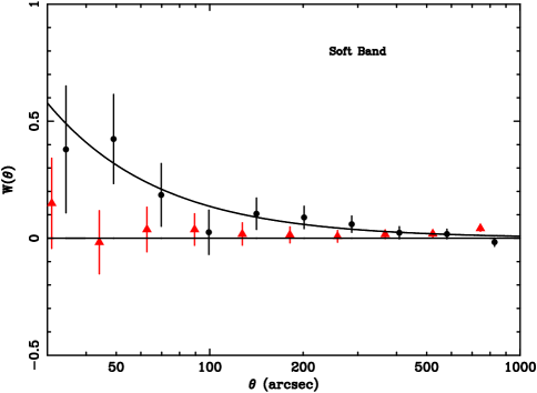
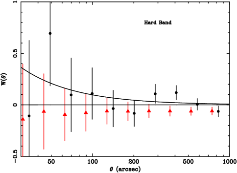
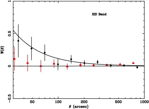
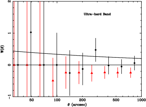
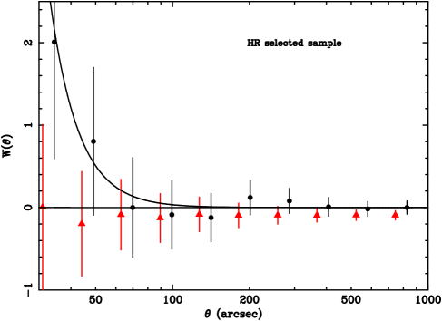
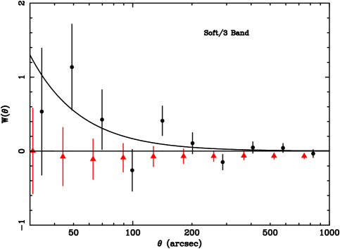
Figure 5: $W(\theta)$ vs. $\theta$ for the soft (top-left), hard (top-right), XID (middle-left), and ultra-hard (middle-right) samples, for a hardness-ratio selected sample (bottom-left) and for a random selection of one third of the soft sources (bottom-right). The solid dots are the integral-constraint-corrected observed values, the grey triangles show the “zero points” from the integral constraint (displaced to the left for clarity), and the solid lines are the best fit $\chi^{2}$ fits to Eq. 5. The middle-right and two bottom panels have different scales on their Y-axis.

6 Looking for source clustering

A survey to detect source clustering requires both depth (to achieve high angular density), and width (to minimise the possibility that a single structure biases the overall average). In practice, a compromise between those two conflicting requirements has to be achieved. The AXIS sample comprises 36 fields outside the Galactic plane, and a relatively high source density (about 35 sources per field, at least in the soft and XID samples), and we have tested what can it say about the angular distribution of sources in the sky.

6.1 Cosmic variance

The simplest test for source clustering is to compare the actual number of sources detected in each field $N_{k}$ with the number expected $\lambda_{k}$ from the best fit log$N$-log$S$ and the sky area of each individual field $\Omega_{k}$ (this is similar to the traditional counts-in-cells method). In principle, if just one field (or a few fields) happens to look through strong cosmic structures, its number of sources should be significantly different from the expected number from a random uniform distribution, as measured by the overall log$N$-log$S$.

The statistics we have used to measure the deviation from such a random uniform distribution are the cumulative Poisson distributions:

$$\begin{array}[]{lcll}P_{\lambda_{k}}(\geq N_{k})&=&\sum_{l=N_{k}}^{\infty}P_{\lambda_{k}}(l)&{\rm if}\,N_{k}>\lambda_{k}\\ P_{\lambda_{k}}(\leq N_{k})&=&\sum_{l=0}^{N_{k}}P_{\lambda_{k}}(l)&{\rm if}\,N_{k}<\lambda_{k}\\ \end{array}$$

where $P_{\lambda}(l)$ is the Poisson probability of detecting $l$ sources when the expected number of sources is $\lambda$. The cumulative distributions above give the probability of finding $\geq N_{k}$ (first row) or $\leq N_{k}$ (second row) sources when the expected number from the source counts is $\lambda_{k}$. This method is similar to the one used in Carrera et al. (Carrera98 (1998)), but in that work we used $P_{\lambda}(l)$ instead of the cumulative probabilities. We believe that the approach used here is a more conservative estimate of how likely is to find a number of sources in a field which is different from the expected value.

The maximum likelihood statistics for the whole sample is then

$$L^{\prime}=\sum_{k}P_{\lambda_{k}}(\geq N_{k})+\sum_{k^{\prime}}P_{\lambda_{k^{\prime}}}(\leq N_{k^{\prime}})$$

, where $k$ runs over the fields for which $N_{k}>\lambda_{k}$, and $k^{\prime}$ over the fields for which $N_{k^{\prime}}<\lambda_{k^{\prime}}$.

We have compared the observed $L^{\prime}$ values in each band with 10000 simulated values, using the values of $\lambda_{k}$ and Poisson statistics. The number of simulations with likelihood values above the observed ones were 1388, 4580, 778 and 4958 for the soft, hard XID and ultra-hard bands, respectively. Nothing significant is found in the hard or ultra-hard samples, while some deviation below or about at the 90% significance level is found in the soft and XID bands. These results, although formally at a low significance, have encouraged us to try more elaborated tests for clustering.

6.2 Angular correlation function

If cosmic structure is present in all (or most) fields, a test for significant deviations from the mean number of sources in each field from some overall average will not give significant results. We should look instead for evidence of sources tending to appear together in the sky with respect to an unclustered source distribution. The classic parametrisation for this effect is the angular correlation function $W(\theta)$ which measures the excess probability of finding two sources in the sky at an angular distance $\theta$ with respect to a random uniform distribution (Peebles Peebles80 (1980)):

$$\delta P=n^{2}\delta\Omega_{1}\delta\Omega_{2}[1+W(\theta)]$$ (3)

where $\delta P$ is the probability of finding two objects in two small angular regions $\delta\Omega_{1}$ and $\delta\Omega_{2}$, separated by an angle $\theta$, when the sky density of objects is $n$.

Since the angular separation is a projection in the sky of the real spatial separations of the sources at different redshifts, the underlying spatial clustering is somewhat blurred with this purely angular measurement. Unfortunately, the more powerful spatial clustering depends on having redshifts for a very high fraction of the sources, or at least knowing precisely what is their redshift distribution. Since none of these two conditions are fulfilled by any of the AXIS samples, we have used the data presently at hand to study the angular correlation function.

There are several proposed ways of measuring the angular correlation function, most of which look for an excess number of source pairs at a given angular separation $\theta$ with respect to a simulated random “uniform” sample (Landy & Szalay Landy93 (1993), Efstathiou et al. Efstathiou91 (1991)). We have chosen the one proposed by Efstathiou et al. (Efstathiou91 (1991)).

$$W(\theta)=f{DD\over DR}-1$$ (4)

where $DD$ is the number of actual pairs of sources with angular separation $\theta$, and $DR$ is the number of pairs of one real and one randomly placed simulated source (see below) at the same separation, while $f$ is a normalisation constant to take into account the different number of real and simulated sources. The error bars around each point are given by $\Delta W(\theta)=\sqrt{(1+W(\theta))/DR}$ (Peebles Peebles80 (1980)).

The “randomly placed” simulated sources have to follow as closely as possible the real distribution of the source detection sensitivity of the survey, giving a “flat” random sky against which to judge the presence (or otherwise) of significant over-densities at different angular separations. We have used bootstrap simulations by forming a pool of real sources with detection likelihoods higher than 15 (our standard value) in the band under study, irrespectively of whether their count rates were above or below the sensitivity map of the corresponding field at the source positions. Then, keeping the number of sources simulated in each field equal to the real number of sources $N_{k}$, we have extracted sources from this pool, keeping their count rates, and their distances to the optical axis of the X-ray telescope, but randomising their azimuthal angle around it. If the source had a count rate above the sensitivity map of the field under consideration at its “new” $(X,Y)$ position, the source was kept in the simulated sample, otherwise a new one is extracted until $N_{k}$ valid simulated sources are found. In this way, the angular distribution of the simulated sources mimics the decline of the source detection sensitivity with off-axis angle. The number of random samples $N_{\rm sim}$ used in each band are shown in Table 8. They have been chosen so as to give a total of about a million simulated sources in each band.

With this recipe, the normalisation constant $f$ above is given by

$$f={\sum_{k}N_{k}\left(N_{k}-1\right)\over 2N_{\rm sim}\sum_{k}N_{k}^{2}}$$

$N_{k}$ being the number of sources in field $k$ and $N_{\rm sim}$ the number of simulations.

If a positive correlation is present at angular scales comparable to the individual field size, the estimate of the mean surface density of objects from the survey is too high, and this causes a negative bias in the angular correlation function known as the integral constraint (Basilakos et al. Basilakos04 (2004)). Given the complicated dependence of the sensitivity over the area of our survey, we have corrected for this effect empirically, finding the angular correlation function that we would have detected in the absence of correlation, via the average of $N_{\rm sim}$ simulated realisations of $W(\theta)$, where the real data were replaced by random samples, simulated independently following the recipe in the previous paragraph. The triangles in Fig. 5 show these “zero points” at each angular scale, which have been used to increase the corresponding observed $W(\theta)$, convolving the error bars using Gaussian statistics.

Applying Eq. 4 to the full sample results in a $\sim$3-$\sigma$ significant bump at about 200 arcsec, which was also present in the simulations, but at lower significance. The bump turned out to be present only in two fields (HD111812 and HD117555), a search in the literature revealed that both fields have stellar clusters in their field of view (Eggen & Iben Eggen89 (1989)). Since we are interested mainly in extragalactic structure, we have opted for excluding these two fields from all subsequent angular clustering analysis, leaving 34 fields.

The $W(\theta)$ obtained in this fashion are shown in Fig. 5, as well as the corresponding best $\chi^{2}$ fits to a power-law model

$$W(\theta)=(\theta/\theta_{0})^{-\gamma}$$ (5)

The best fit parameters for this model are given in Table 8. In that Table we also give the significance of the detection from an F-test comparing the $\chi^{2}$ value of the power-law model with a simple $W(\theta)=0$ no-clustering model. The F-test suggests significant correlation in the soft and XID bands at the $\sim$99% level. The lack of significant detections in the two harder bands might be due to the lower number of sources with respect to the soft and XID bands (see below).

Gandhi et al. (Gandhi06 (2006)) also found significant angular correlation in the XMM-LSS sample in the soft band, with a similar slope ($\gamma=1.2\pm 0.2$), and a lower correlation length ($\theta_{0}=7\pm 3$ arcsec), but still compatible with ours within $\sim$1-$\sigma$. Vikhlinin & Forman (Vikhlinin95 (1995)) found $\gamma=0.7\pm 0.3$ and $\theta_{0}=4\pm 3$ arcsec, again a lower correlation length than us, but compatible within less than 1-$\sigma$ with our $\gamma\equiv 0.8$ result. On the other hand, Basilakos et al. (Basilakos05 (2005)) also found significant angular correlation in this band, but with a higher correlation length ($\theta_{0}=10.4\pm 1.9$ arcsec, with the canonical slope), just compatible with our results at about the 2-$\sigma$ level. Basilakos et al. (Basilakos05 (2005)) also used Limber’s equation (Peebles Peebles80 (1980)) to calculate the spatial correlation function from the angular correlation function, assuming several different AGN X-ray luminosity functions (since most X-ray sources at low flux levels are expected to be AGN). Their high correlation lengths are only compatible with AGN optical (e.g. Croom et al. Croom02 (2002), Grazian et al. Grazian04 (2004)) or X-ray correlation functions (Carrera et al. Carrera98 (1998), Akylas et al. Akylas00 (2000), Mullis et al. Mullis04 (2004)) if the clustering is constant in physical coordinates, while optical QSO clustering seems instead to be constant in comoving coordinates (Croom et al. Croom01 (2001), but see also Grazian et al. Grazian04 (2004), Croom et al. Croom05 (2005)). Akylas et al. (Akylas00 (2000)) also found significant angular correlation in the soft band sources in the RASS-BSC, but at much higher angular distances ($\sim 8^{\circ}$).

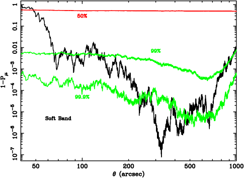
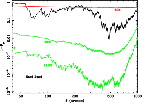
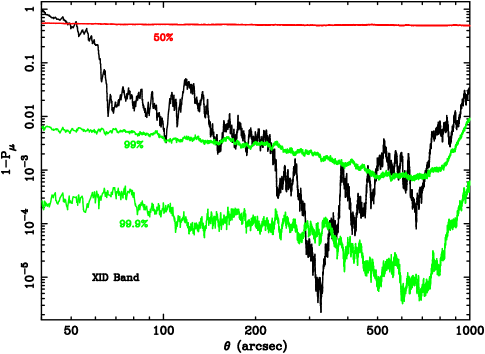
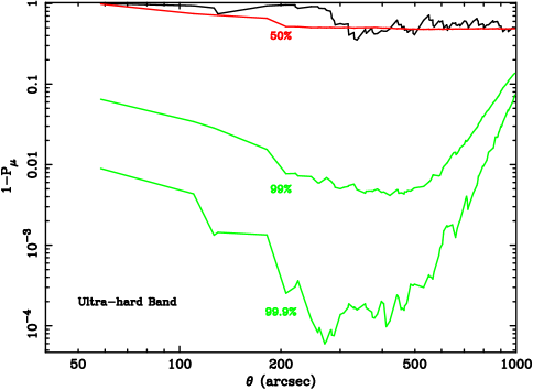
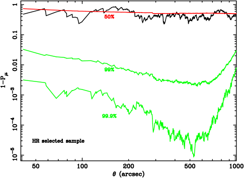
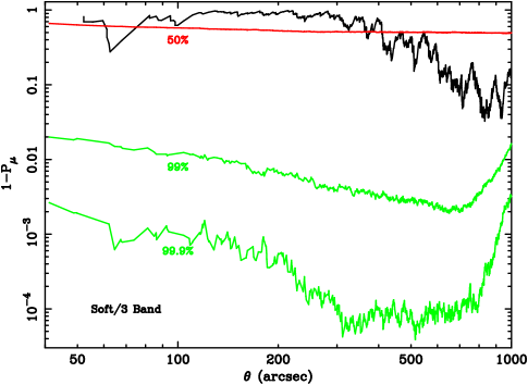
Figure 6: $1-P_{\mu}(N_{\theta})$ vs. $\theta$ for the soft (top-left), hard (top-right), XID (middle-left), ultra-hard (middle-right) selected samples, for a hardness-ratio selected sample (bottom-left) and for a random selection of one third of the soft sources (bottom-right). The median (50%), 99% and 99.9% levels from random simulations are also shown (grey jagged lines). The Y-axis scaling is different in different panels, and has been chosen for maximum clarity.

Correlation of hard band selected sources is not detected by Gandhi et al. (Gandhi06 (2006)) (413 sources) and Puccetti et al. (Puccetti06 (2006)) (205 sources). However, clustering is very significantly detected ($>4\sigma$) by Basilakos et al. (Basilakos04 (2004)) (171 sources) with $\gamma=1.2\pm 0.3$ and $\theta_{0}=49^{+16}_{-25}$ arcsec. Clustering is also detected at similar significance by Yang et al. (Yang03 (2003)), with $\theta_{0}=40\pm 11$ arcsec (for $\gamma\equiv 0.8$) for 278 sources. This is somewhat surprising since the Basilakos et al. sample has less than half the number of sources than Gandhi et al., and a similar number of sources to Puccetti et al., and the Yang et al. sample is again smaller than the Gandhi et al. sample. Our angular correlation length is compatible with the Basilakos et al. (Basilakos04 (2004)) (and with the Puccetti et al.) result within 1-$\sigma$, but not with the Yang et al. correlation length. However, the F-test on the correlation function, and the superior $P_{\lambda}(N)$ test (see below and Fig. 6) do not detect clustering. Again, our sample seems to give somewhat intermediate results in between those of Basilakos et al. (Basilakos04 (2004)) and Yang et al. (Yang03 (2003)) on one hand, and Gandhi et al. (Gandhi06 (2006)) and Puccetti et al. (Puccetti06 (2006)) in the other.

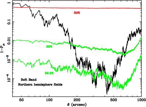
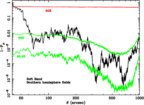
Figure 7: $1-P_{\mu}(N_{\theta})$ vs. $\theta$ for the soft band and for the fields in the northern (left) and southern (right) Galactic hemispheres. The median (50%), 99% and 99.9% levels from random simulations are also shown (grey jagged lines).

Since each bin in $W(\theta)$ contains information from many pairs, perhaps involving the same real and simulated sources many times, it is at least debatable whether the hypothesis of independent bins underlying the $\chi^{2}$ test applies in this case. To circumvent this problem, we have applied a simple test for the significance of the correlation, using Poisson statistics to compare the expected number of pairs (at distances smaller or equal than each individual observed distance) in absence of correlation ($\mu=\sum_{\theta^{\prime}<\theta}DR(\theta^{\prime})/f$) with the number of observed pairs ($N_{\theta}=\sum_{\theta^{\prime}<\theta}DD(\theta^{\prime})$). The quantity $1-P_{\mu}(N_{\theta})$ versus the angular distance $\theta$ is shown in Fig. 6 for each band. We can estimate the “signal” in the absence of correlation (similarly to what we have done to quantify the integral constraint) repeating this exercise, but replacing the real data by randomly placed sources (see above). For each sample we have performed 10000 simulations along these lines. In this way, we have for each angular scale and sample the distribution of the expected value of $1-P_{\mu}(N_{\theta})$ if the sources are not correlated. We show in Fig. 6 the median and the upper 99% and 99.9% percentiles of those distributions for each angular scale. The simulations show clearly that the detection significance is actually lower than the value given purely by Poisson statistics, when there are more than $\sim$1000 sources, as in the soft and XID bands, where the 99% percentile is around the Poisson 3-$\sigma$ level. While in the hard and ultra-hard bands the 99% percentile is around the “right” Poisson position, albeit with large excursions.

Using the percentiles from the simulations, we have found a $>99$% (but mostly $<$99.9%) significant detection of correlation in the angular positions of in our soft sample at separations 200-700 arcsec. In the XID band the significance is lower, at just about 99% significance, with essentially one peak of higher significance at $\sim$300 arcsec. In contrast, no signal is found in either the hard or ultra-hard bands. The lack of significant detections in the two harder bands might be due to the lower number of sources with respect to the soft and XID bands.

We have performed a test for the influence of the number of sources in the detection of clustering, since we only detect clustering in the samples with more than 1000 sources. We have rejected at random two of every three sources in the soft band sample, and repeated both tests for correlation: the clustering signal disappears (see Table 8, Figs. 5 and 6). We have also repeated this test keeping at random one half and two thirds of the soft sources, only finding correlation at the 99% level in the last case. We conclude that clustering in the hard and ultra-hard bands may be as strong or stronger than clustering in the soft band, but our relatively low number of sources prevents us from detecting it. This is compatible with the results of Gilli et al. (Gilli05 (2005)), which do not find any significant difference between the clustering properties of soft or hard X-ray selected sources in the CDF.

The significant clustering found with the $P_{\mu}(N_{\theta})$ of the soft band corresponds to a broad bump between about 150 and 700 arcsec, with “peaks” at about 300, 400 and 650 arcsec (the first two are significant even at the 99.9% level). These “peaks” also appear to be present in the XID band. While the increase in the number of real pairs giving rise to the broad bump is very gradual, the “peaks” must correspond to significant increases in relatively narrow ranges of angular distances. To investigate if these “peaks” come from a small number of fields in a particular region of the sky, we have divided the sample between the fields in the northern and southern Galactic hemispheres. The $1-P_{\mu}(N_{\theta})$ for these regions are shown in Fig. 7. Despite the lower significances (expected because of the lower numbers of sources), the broad bump and the peaks are still present in the samples from the two hemispheres, the $\sim$300 arcsec peak being common to both, with the one at 400 arcsec appearing predominantly in the northern hemisphere, and the one at 650 arcsec in the southern hemisphere. We have also repeated the analysis excluding the two fields with obvious cluster emission (A1837 and A399) from the northern and southern Galactic hemisphere sub-samples, respectively, finding no significant differences in the strength or position of the “peaks”. As a further test, we have looked for signal in the 7 deeper fields (Texp$>$40 ks, $\sim$400 sources) and in the remaining 27 fields ($\sim$800 sources), finding it only in the latter, and hence the signal is not due to a few deep fields.

A detailed discussion of the (cosmic or statistical) origin of these structures is outside the scope of this paper, and will be discussed with a larger sample elsewhere. However, whatever the origin of the angular structure we have found, it must be relatively widespread over the data and/or the sky. We take this to mean that, if it has a real cosmic origin, it must come from sources at $z\leq 1.5$, which is the peak of the redshift distribution of medium depth X-ray surveys (Barcons et al. Barcons06b (2007)).

6.3 Angular correlation of a hardness-ratio-selected sample of sources

A low significance or absence of correlation in the hard band is somewhat surprising, since most sources at the flux levels of our sample are AGN (Barcons et al. Barcons06b (2007)), which are known to cluster strongly (both X-ray selected -Mullis et al. Mullis04 (2004), Yang et al. Yang06 (2006)- and optically selected -Croom et al. Croom05 (2005)-). Furthermore, obscured AGN appear more commonly in hard X-ray selected samples (Della Ceca et al. DellaCeca06 (2006), Caccianiga et al. HBS28 (2004), Della Ceca et al. DellaCeca04 (2004), Barcons et al. Barcons06b (2007)).

Gandhi et al. (Gandhi06 (2006)) have found that, despite the absence of significant angular correlation in their hard sample, if they select only the hardest spectrum sources (using the soft-to-hard hardness ratio), and they use lower significance sources, the significance of the correlation increases to $\sim 2-3\sigma$. They lowered their significance level in order to increase the number of sources in the tested sample. This significant correlation only in the hardest of the hard-X-ray-selected sources is a very intriguing and potentially interesting result.

We have done a similar analysis, defining the same hardness ratio $HR=(H-S)/(H+S)$ where $H$ and $S$ are the 2-12 keV and 0.5-2 keV count rates, respectively. We have selected the sources detected in either the soft or hard bands (in the sense explained in Section 2.4) which have $HR\geq-0.2$ (Gandhi et al. Gandhi06 (2006)).

The F-test seems to indicate correlation at $>99$% level (Table 8), but the superior Poisson method (Fig. 5) does not detect clustering on any angular scales, with the data being actually consistent with the median of the random simulations. We cannot thus confirm the results of Gandhi et al. (Gandhi06 (2006)), despite having a slightly larger sample of sources (250 versus their 209). This is compatible with the results of Yang et al. (Yang06 (2006)) which do not find any significant differences between the spatial clustering of sources with soft or hard spectra.

7 Conclusions

We present the results from AXIS (An XMM-Newton International Survey) which comprises 1433 distinct serendipitous X-ray sources detected with a likelihood of 15 ($\sim$5-$\sigma$) in XMM-Newton EPIC pn observations in 36 different XMM-Newton observations at high Galactic latitude. We have defined sub-samples in four bands: 0.5-2 keV(soft, 1267 sources), 2-10 keV (hard, 397 sources), 0.5-4.5 keV (XID, 1359 sources) and 4.5-7.5 keV (ultra-hard, 91 sources). The first two being the “standard” X-ray bands, the third one chosen to span the energy range with the best sensitivity of that camera, and the last one taking advantage of the unprecedented hard X-ray sensitivity of XMM-Newton above 4 keV. Given the distribution of exposure times of the fields selected for AXIS, it will serve as a pathfinder to the X-ray and optical properties of the sources in large scale XMM-Newton catalogues (1XMM, 2XMM, $\ldots$).

Using count rates in the 5 standard XMM-Newton bands as low-resolution spectra we have fitted single power-laws to all sources in the XID and hard bands independently, in order to calculate source fluxes without assuming a constant spectrum (see Table 4). Our internal and external checks make us confident on the results from this technique. The average best fit power-law slope in the XID band is $\langle\Gamma\rangle\sim 1.8$, independently of the sample to which the sources belong, while the average is $\langle\Gamma\rangle\sim 1.5-1.6$ in the hard band.

We have constructed empirical sensitivity maps in the four bands, taking into account the exposure maps, the background maps and the excluded regions (see Table 1). We have derived sky coverages as a function of flux in the four bands, taking into account the distribution of spectral slopes of the sources. The total area covered is 4.8 deg² (see Fig 1).

Our data have been combined with both wider and shallower (BSS/HBSS, Della Ceca et al. DellaCeca04 (2004), AMSS, Ueda et al. Ueda05 (2005)), and narrower and deeper (CDF, Bauer et al. Bauer04 (2004)) surveys to measure the X-ray source counts over as wide flux range as possible, reaching 4 orders of magnitude in the soft band ($\sim$2000 sources), $\sim$3 in the hard and XID bands ($\sim$800 and $\sim$1800 sources, respectively), and a bit more than 1 in the (largely unexplored) ultra-hard band ($\sim$140 sources). Data from different observatories and instruments are mutually compatible, allowing the joint analysis of the source counts.

We have performed maximum likelihood fits to a broken power-law model for the log$N$-log$S$ in the four bands (see Table 5). We have found that fits to the source counts using fixed spectral slopes produce similar results to those using individual source spectral slopes (as we have done here), but give rise to larger error bars. The source counts in the soft, hard and XID bands show breaks at fluxes $\sim 10^{-14}$ cgs. Detailed examination of the ratios between the data and that simple model in the soft and XID band do not show any significant differences, while in the hard band there seems to be evidence for a further flux break at $\sim 3\times 10^{-15}$ cgs and several changes of slope. Since this is only present in the hard band, it is difficult to assess whether this behaviour is due to a too simple characterisation to contributions from different populations at different redshifts, or it is due to calibration uncertainties. Future large scale XMM-Newton catalogues (such as 2XMM) will be useful to address this question. The best fit model parameter values are compatible with previous smaller or similar surveys, but our combination of large number of sources and wide flux coverage produce in general smaller uncertainties in the best fit parameters.

We have used our best fit log$N$-log$S$ parameters to calculate both the total resolved fraction of the XRB (including the contribution from sources a bright fluxes, see Table 6), and the relative contribution of different flux bins to the XRB (see Fig. 4). We have used the estimates of the average XRB intensity in the soft and hard bands from Moretti et al. (Moretti03 (2003)), translating them to the XID and ultra-hard bands using $\Gamma=1.4$ (Marshall et al. Marshall80 (1980)). The total resolved fraction down to the lowest fluxes of the combined sample reaches 87% in the soft band and 85% in the hard band, where we have been able to reach deep fluxes using pencil beam surveys (Bauer et al. Bauer04 (2004)), but it is only $\sim$60% in the XID band and about 25% in the ultra-hard band. The total intensity produced by extrapolating our best fit soft and hard log$N$-log$S$ to zero flux is insufficient to saturate the XRB intensity. Assuming a second flux break just below our minimum detected fluxes, we have estimated the minimum slope below this break necessary to produce the whole XRB with discrete sources, getting 1.85 (1.84) in the soft (hard) band. Comparing these slopes with those of the fainter galaxy and AGN source counts from the CDF (Bauer et al. Bauer04 (2004)), reveal that galaxies could easily provide this re-steepening, while among AGN only perhaps the absorbed ones could just about do it.

The maximum fractional contribution to the XRB in the soft, hard and XID bands comes from sources within a decade of $10^{-14}$ cgs (which is about where the break flux for the broken power-law lies). This fractional contribution reaches about 50% of the total in the soft and hard bands. Medium depth surveys such as AXIS (and indeed the 1XMM catalogue, and its successor 2XMM) therefore are instrumental in understanding the evolution of the X-ray emission in the Universe, at least up to 10 keV.

Hickox & Markevitch (HM06 (2006)) have recently re-estimated the soft and hard XRB intensities using CDF data, finding lower resolved fractions of the XRB than our (and previous) estimates. We have found that the difference with our results in the soft band (where it is highest) is only at the $\sim$1-$\sigma$ level, and it is mainly due to the different ways in which the total XRB intensity is calculated. HM06 add different contributions at different fluxes, which produces an “effective” spectral shape of the XRB ($\Gamma\sim 1.8$) which is much steeper than the “canonical” XRB spectral slope of $\Gamma=1.4$ (which we have assumed). We have shown that the difference between both estimates of the soft XRB intensity cannot be removed just by relaxing our assumption. The HM06 intensity from resolved sources is very similar to ours. Converting our results to 1-2 keV, the difference with HM06 all but vanishes.

After excluding two fields in which there is evidence for the presence of stellar clusters, we have used the AXIS sources to study the presence of cosmological structure in the X-ray sky, through the cosmic variance in the number of sources per field, and the distribution of the angular separations of the sources. The first one is in principle more sensitive to the presence of significant over-densities in a few fields, while the second looks for an overall angular clustering of sources. No cosmic variance is detected at all in the hard and ultra-hard bands, while some signal at about the 90% level is present in the soft and XID bands, probably because they are the ones with the larger number of sources. Angular clustering is studied in two ways. The first one is the angular correlation function $W(\theta)$. Using this method, we detect signal at about the 99% level in the soft and XID bands, but not in the hard and ultra-hard bands (Table 8 and Fig. 5). The strength of the clustering signal we have found is intermediate between those of previous results (e.g. Gandhi et al. Gandhi06 (2006), Basilakos et al. Basilakos04 (2004), 2005, Vikhlinin & Forman Vikhlinin95 (1995)).

A formally more appropriate method using Poisson statistics detects clustering at the 99-99.9% level in the soft and XID samples, but not in the hard or ultra-hard bands (Fig. 6). Repeating the test for a randomly 1-in-3 selected sample of soft sources completely destroys the clustering signal, which we take to imply that there might be a “real” angular clustering among hard sources which we have failed to detect due to the small number of sources. Dividing the soft sample in several sub-samples reveals that the signal is widespread over the sky, and not limited to a few deep fields. This means that, if it has a cosmic origin, it must come from $z\leq 1.5$, the peak of the redshift distribution of medium flux X-ray surveys (Barcons et al. Barcons06b (2007)). We cannot confirm the detection of signal among hard-spectrum hard sources reported by Gandhi et al. (Gandhi06 (2006)).

Appendix A Empirical sensitivity maps

The present version of esensmap (the SAS task to calculate sensitivity maps for the EPIC cameras on board XMM-Newton) assumes pure Poisson statistics to evaluate the detection sensitivity at different positions in the field of view. Since the detection of the sources and the determination of their parameters is a complicated process, which includes how well does the profile of the count rates match the PSF, the result is bound to deviate from the naïve assumption of pure Poisson statistics.

We have followed an empirical approach, looking for a simple relationship between the observed EPIC pn count rates of the detected sources in each band $cr$ (in cts/s, columns RATE in the SAS source lists), and the pure Poisson count rate $crpoisim$ (in cts/s) as calculated from the total number of background counts $bgdim$ within a circle of radius $cutrad$ (related to the column labelled CUTRAD in the SAS source lists, and given in units of 4^′′ pixels) around the source position, the detection likelihood of the source $L$ (columns labelled DET_ML in the SAS source lists), and the average value of the exposure map (in seconds) within that radius $expim$, so that

$$-log(P_{bgdim}(>(bgdim+crpoisim\times expim))=L$$ (6)

with $P_{\lambda}(>N)$ as defined in Eq. 6.1.

The values of CUTRAD are in principle different for each source in each field, since they are chosen by emldetect to maximise the signal-to-noise ratio for source detection. We have found that there is no significant correlation between CUTRAD and either the off-axis angle of the source, RATE or BG_MAP (the average background value in counts per pixel within the extraction circle), and therefore we have adopted for $cutrad$ in each band the average of CUTRAD for the sources having $L$ between 8 and 20 in that band. We have checked that there is no significant difference in the goodness of the fits below between using the actual CUTRAD value for each source or the average $cutrad$.

$expim$ above is the average of the exposure map within a circle of radius $cutrad$ around the X-ray source positions. The exposure maps for the single bands are PPS products. We have created exposure maps for the composite bands using the SAS task eexpmap, which generates exposure maps for the energy in the middle of the PI interval, which could be inaccurate for wide bands. To assess the effect of this approximation we have also calculated “average” exposure maps in the composite bands, weighting the single band exposure maps with the counts in the images pixel by pixel. Again, there are no significant differences between the results from those two types of exposure maps.

Unfortunately, the background files are not PPS products. We have generated them from the individual and composite bands using the SAS task esplinemap, which excludes areas around the sources in an input source list, and fits the remaining background using a spline (with 16 nodes in our case). We have then calculated $bgdim$ by summing the values of the background image over a circle of radius $cutrad$.

We show in Fig. 8 plots of RATE versus $crpoisim$ for the single and composite bands, along with the best linear fit model (RATE$=LI\times crpoisim$), for sources having $8\leq L\leq 20$ in each band. The best fit $LI$ along with the values of $cutrad$ for each band are given in Table 9. From the number of sources in each fit and the values of the $\chi^{2}$ it is clear that the fits are quite good, and more sophisticated models are not needed. The values of $LI$ are all within $\sim$10% of 1, implying that the correction is small (as expected), but from the improvement of the $\chi^{2}$ values from using $LI\equiv 1$ (which is equivalent to RATE$\equiv crpoisim$), we conclude that it is also highly significant.

The recipe for creating a sensitivity map is then:

1. Create background and exposure maps

2. Chose a likelihood value $L$ for the significance of the detections. This recipe has only been tested for $8\leq L\leq 20$, but it could be in principle valid for likelihood values outside this interval.

3. Choose a source extraction radius $cutrad$ appropriate for the band you are interested in (Table 9)

4. For each pixel $(X,Y)$ in your input image:

   1. Calculate the sum of the values of the pixels in the background map whose centres are within $cutrad$ of $(X,Y)$: $bgdim$

   2. Calculate the average of the values of the pixels in the exposure map whose centres are within $cutrad$ of $(X,Y)$: $expim$

   3. Find $ctspoisim$ such that $-\log(P_{bgdim}(>(ctspoisim+bgdim)))=L$

   4. Calculate $sens(X,Y)=ctspoisim/expim\times$LI.

5. $sens(X,Y)$ is our empirical estimate of the typical count rate of a source at $(X,Y)$ detected with likelihood $L$

Table 9: Summary of the results of the linear fits of $crpoisim$ to RATE: Band is the band used for the fit, $cutrad$ is the source extraction radius (in units of 4^′′ pixels), $LI$ is the best fit multiplying constant, $N$ is the number of sources in the fit, $\chi^{2}_{LI}$ is the $\chi^{2}$ value of the best linear fit, while $\chi^{2}_{0}$ is the $\chi^{2}$ of the fit to $LI\equiv 1$, and $P(F)$ the F-test probability of letting $LI\neq 1$ not being a significant improvement in the fit

Band	$cutrad$	$LI$	$N$	$\chi^{2}_{LI}$	$\chi^{2}_{0}$	$P(F)$
	(pixels)
1	5.12	1.14	284	104.5	185.5	$<10^{-6}$
2 (soft)	5.08	1.10	653	140.1	226.0	$<10^{-6}$
3	5.15	1.14	414	105.7	208.4	$<10^{-6}$
4 (ultra-hard)	5.49	1.14	127	25.7	56.2	$<10^{-6}$
5	5.86	1.15	16	1.7	5.5	$<10^{-4}$
9 (XID)	5.04	1.02	722	141.0	145.2	$<10^{-5}$
3-5 (hard)	5.18	0.89	243	176.2	237.8	$<10^{-6}$

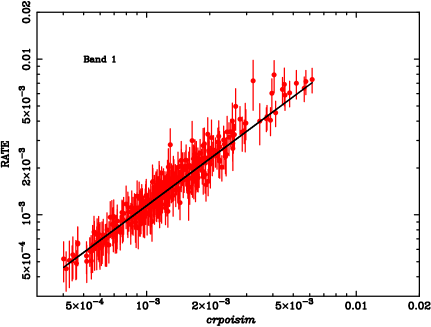
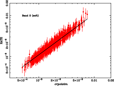
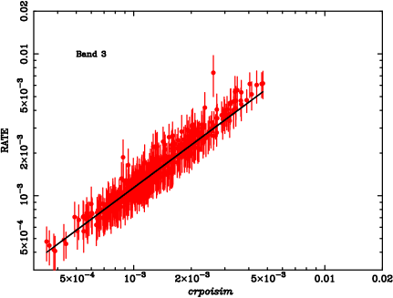
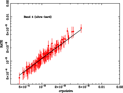
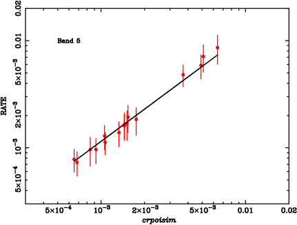
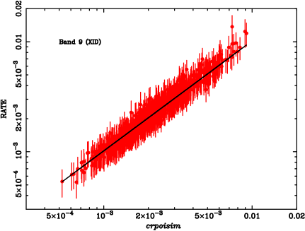
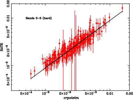
Figure 8: RATE vs. $crpoisim$ for all bands. Also shown are the best linear fits.

Appendix B Evaluating the count rate spectral fit

To check the validity of our procedure we have performed both internal and external tests. The simplest internal check is to simulate sources with a single spectral slope ($\Gamma=2$ in our case), fit them, and compare the output slope values to the input value. We have kept the total (0.5-10 keV) count rates of the sources fixed to the observed count rates, and simulated the count rates in each band using a Poisson deviate from the expected number of counts for the fixed slope and the exposure times $T_{\rm exp}$ in Table 1. The error on the simulated count rates ($\Delta CR$) were a bit more delicate to estimate. Using simply $\Delta CR=\sqrt{CR/T_{\rm exp}}$ would not be adequate, because it does not include the contribution from the background subtraction, and because the statistics of the source detection by emldetect are very close to, but not exactly, Poissonian. We have used the selected sources to look for an empirical relationship between the observed $\Delta CR$ and the naive $\sqrt{CR/T_{\rm exp}}$. We have found that a linear relationship is a good visual fit, with the parameters given in Table 10. This is the recipe we have used to simulate the errors in the count rates in our simulations. The weighted averages of the fitted slopes are given in Table 11, showing that any internal deviations are small ($<0.1$), and that there are no obvious biases for sources selected in different bands. We have repeated the simulations for $\Gamma\equiv 1.8$ and $\Gamma\equiv 1.7$, with similar results and conclusions.

Table 10: Empirical relationship between the observed errors on the count rates $\Delta CR$ and the naive $\sqrt{CR/T_{\rm exp}}$. We give the parameters $a$ and $b$ of a linear relation $\Delta CR=a\times\sqrt{CR/T_{\rm exp}}+b$

band	$a$	$b$
2	1.597	-
3	1.419	$3.824\times 10^{-5}$
4	1.452	$6.166\times 10^{-5}$
5	2.350	$1.184\times 10^{-4}$

We have also performed an external check against the single power law fits to the “properly” extracted spectra by Mateos et al. (2005). In that work the fits were done using xspec with response matrices and effective areas generated for each source with the corresponding SAS tasks. Since the Mateos et al. (2005) spectra were extracted between 0.2 and $\sim$12 keV, we have fitted our sources using bands 2, 3, 4, and 5. In Fig. 9 we show their best fit single power law slopes vs. our best fit slopes for the common accepted sources (a total of 1143 sources, which include some sources fitted by Mateos et al. but not included in their paper, Mateos private communication). The best $\chi^{2}$ fit proportionality constant using errors in both the X and Y axis is 0.980$\pm$0.003. This result makes us confident in our fitting method, showing that we haven’t missed significant effects that were not already corrected in the emldetect count rates. A number of sources deviate appreciably from the 1:1 relation in Fig. 9, the effect being more noticeable to the eye for values of $\Gamma_{\rm 0.2-12\,keV}$ between about 1.7 and 3. Within that interval, the number of sources with $\Gamma_{\rm 0.5-10\,keV}>3$ is only 14% of the total number of sources in that interval, this simple test already indicates that the number of sources with pathological spectral fits is a small minority. We will discuss the influence of these sources in more detail below. We show in Fig. 10 our best fit slopes versus our 0.5-12 keV count rates. There are some sources with very steep fitted slopes (because they have only been significantly detected in one band), but the bulk of our sources have reasonably “standard” spectral slopes, with no significant trends towards too steep or too faint slopes at lower count rates.

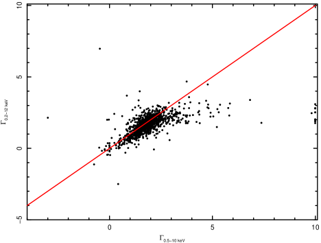
Figure 9: Full band power-law slope from Mateos et al. (2005) vs. our 0.5-10 keV slope for the common accepted sources. The solid line shows the 1:1 relation.

Figure 10: Our 0.5-10 keV slope versus the 0.5 to 12 count rate for our 1433 sources.

Individually the fits are therefore good, but we have also assessed whether there are significant biases in the average slope, and whether the error bars on the slopes are adequate. We have first studied the distribution of the differences between the slopes divided by the quadratic sum of the errors (which would be expected to follow a $N(0,1)$ distribution in the Gaussian case). There is a small bias in these “normalised” differences of $\sim$20% of the combined error bar (such us we tend to find steeper slopes than Mateos et al.), with a significant dispersion above the expected value. Fitting a Gaussian to this distribution (which is not a Gaussian) finds a similar central value, but a much smaller dispersion, indicating that much of the excess variance is due to a limited number of significant outliers.

Assuming Gaussian statistics, the error on the mean can be obtained dividing the standard deviation by the square root of the number of sources ($\sim$1000 in our case). If we perform this calculation for our normalised differences, the value is much smaller than the $\sim$20% relative bias above, which means that the bias is significant (many times the “error on the mean”), despite its low relative value.

Studying the distribution of the absolute differences between the slopes (without dividing by the combined error bar), again there is a bias towards softer slopes in our sample of $\Delta\Gamma\sim$0.12, with a very significant dispersion, which again is much reduced in the Gaussian fit. Our conclusion is similar to above.

If we compare our weighted average slopes with Mateos et al, there is also a difference, but in the sense of our slopes being flatter than theirs. Since the weighted average essentially discards the sources with large error bars, this means that some of the outliers discussed above are soft sources with large error bars which bias the arithmetic average towards softer slopes.

Table 11: Number of sources selected in different bands $N$, weighted average slopes $\langle\Gamma\rangle$ and errors (taking into account both the error bars in the individual $\Gamma$ and the dispersion around the mean), and number of sources used in the average $N_{\rm ave}$, for the simulated sources (see Section 3). The soft, hard, XID and ultra-hard bands are as defined in the text. “Soft and hard” refers to sources selected simultaneously in the soft and hard bands, “Only soft” refers to sources selected in the soft band but not in the hard band, and “Only hard” refers to sources selected in the hard band and not in the soft band

		0.5-2 keV			2-10 keV
Selection	$N$	$N_{\rm ave}$	$\langle\Gamma\rangle$		$N_{\rm ave}$	$\langle\Gamma\rangle$
Soft	1267	1267	2.008$\pm$0.004		1259	2.029$\pm$0.007
Hard	397	397	2.008$\pm$0.005		396	2.039$\pm$0.010
XID	1359	1359	2.007$\pm$0.004		1352	2.030$\pm$0.007
Ultra-hard	91	91	2.014$\pm$0.008		91	2.019$\pm$0.013
Soft and hard	345	345	2.009$\pm$0.005		345	2.038$\pm$0.010
Only soft	922	922	2.007$\pm$0.006		914	2.005$\pm$0.013
Only hard	52	52	1.99 $\pm$0.03		51	2.10 $\pm$0.05