Microscopic Diffusion in Stellar Evolution Codes: First Comparisons results of ESTA-Task 3

Abstract

We present recent work undertaken by the Evolution and Seismic Tools Activity (ESTA) team of the CoRoT Seismology Working Group. The new ESTA-Task 3 aims at testing, comparing and optimising stellar evolution codes which include microscopic diffusion of the chemical elements resulting from pressure, temperature and concentration gradients. The results already obtained are globally satisfactory, but some differences between the different numerical tools appear that require further investigations.

1 Introduction

In previous papers we have presented the work undertaken by the Evolution and Seismic Tools Activity (ESTA) team of the CoRoT Seismology Working Group (see Monteiro et al. [2006] and references therein). In this activity, our main goal is to test, compare and optimise numerical tools which will be used to model the internal structure and evolution of the CoRoT target stars and to calculate their oscillation properties.

ESTA-Task 1 is now finished, it has concentrated on the comparison of standard stellar models coming from seven stellar evolution codes in the range of mass (from $0.9$ to $5.0$ ${\mathrm{M}}_{\odot}$) and evolution stages (from the pre-main sequence to the subgiant branch) to be covered by the CoRoT main targets. Task 2, still underway, has concentrated on seismic codes (see Moya [2007]). The results so far obtained in Tasks 1 and 2 are quite satisfactory, showing minor differences between the different numerical tools provided the same assumptions on the physical parameters are made. These first comparison steps have given us confidence on the numerical tools that will be available to interpret the future CoRoT seismic data.

We present here the new ESTA-Task 3 devoted to the comparison of stellar models taking into account microscopic diffusion of chemical elements resulting from pressure, temperature and concentration gradients (see Thoul & Montalbàn [2007]). In this step, we do not take into account diffusion due to the radiative forces, nor the extra-mixing of chemical elements due to differential rotation or internal gravity waves (see Alecian [2007]; Mathis [2007]; Zahn [2007]).

Evolution models of 1.0, 1.2 and 1.3 ${\mathrm{M}}_{\odot}$ have been calculated by the ESTA group with different stellar evolution codes up to the subgiant branch. We present the first comparisons of those stellar models at particular stages of the evolution. Detailed comparisons of some of the codes and discussions of models are presented by Montàlban et al. ([2007]), Christensen-Dalsgaard([2007]), Marconi ([2007]) and Christensen-Dalsgaard & Di Mauro ([2007]).

2 Specifications of ESTA-Task 3

2.1 Input physics

The physical assumptions proposed as the reference for the comparisons are the same as used for Task 1 and no overshooting and are described in Monteiro et al. ([2006]). Regarding diffusion, we focus on helium and heavy element diffusion due to pressure, temperature and concentration gradients.

As reviewed by Thoul & Montalbàn ([2007]), two approaches to obtain the diffusion equation from the Boltzmann equation for binary or multiple gas mixtures can be followed: one is based on the Chapman-Enskog theory (Chapman & Cowling [1970], hereafter CC70) and the other on the resolution of the Burgers equations (Burgers [1969], hereafter B69). In both methods, approximations have to be made to derive the various coefficients entering the diffusion equations, in particular the diffusion velocities which are written as a function of the collision integrals. In the stellar evolution codes which have participated to Task 3, either the CC70 or the B69 approach has been used (see Section 2.3 below).

Table 1: Specification of the models. Left: The three cases with corresponding masses and initial chemical composition. Right: The three evolutionary stages examined for each case. Phases A and B are respectively in the middle and end of the M–S stage. Phase C is on the subgiant branch. $X_{c}$ denotes the central H abundance in mass fraction and the He core is defined as the region of the star where the H abundance $X$ is lower than 0.01.

case	$\frac{M}{M_{\odot}}$	$Y_{0}$	$Z_{0}$
3.1	1.0	0.27	0.017
3.2	1.2	0.27	0.017
3.3	1.3	0.27	0.017

phase	$X_{c}$	$M_{\mathrm{He\ core}}$
A	0.35	-
B	0.01	-
C	0.00	0.05$M_{\mathrm{star}}$

2.2 Cases for model comparison

During the $10^{\mathrm{th}}$ CoRoT Week in Nice we defined 3 cases (i.e. three values of the stellar mass) for the models to be compared under Task 3 (Lebreton [2006]). These cases are presented in Table 1. We chose rather low values of the masses (i.e. $M<1.4M_{\odot}$) for which diffusion resulting from radiative forces can be neglected. Furthermore, this avoids the problems occurring at higher masses where the use of microscopic diffusion alone produces a very important depletion of helium and heavy elements at the surface (and a concomitant increase of the hydrogen content) and in turn requires to invoke other mixing processes to control the gravitational settling (see for instance Turcotte et al. [1998]). For each case, models at different evolutionary stages have been considered. We focused on three particular evolution stages : middle of the main-sequence (M–S), end of the M–S, subgiant branch.

2.3 Participating stellar internal structure and evolution codes

Up to now six stellar evolution codes have been involved in Task 3. We give below brief information on the way diffusion has been implemented in each of them. More details can be found in Monteiro et al. ([2006]) and references therein as well as in the presentations made during the Joint HELAS-CoRoT Workshop which can be downloaded at the Web site http://www.astro.up.pt/investigacao/conferencias/hce2006/.

• ASTEC – Aarhus Stellar Evolution Code: In ASTEC diffusion is treated according to the simplified Michaud & Proffitt formalism ([1993], hereafter MP93) based on the B69 approach in which the heavy elements are treated as trace elements (see Christensen-Dalsgaard [2007]). Models with either pure He diffusion or He-Z diffusion have been calculated (hereafter ASTEC-He and ASTEC-He-Z models). In the latter case all heavy elements are represented by ${\mathrm{{}^{16}O}}$. Models have 1242 mesh points and the number of time steps to reach phase C is in the range 200-2000 depending on the model.

• CESAM – Code d’Évolution Stellaire Adaptatif et Modulaire: Two formalisms for diffusion have been implemented in the CESAM2k code: the simplified MP93 formalism and a general formalism based on the resolution of Burger’s equations and the Paquette et al. ([1986]) collision integrals (Morel [1997]; Lebreton [2007]). In the present models He and seven heavy elements have been followed explicitly and the ionisation degree of each species has been calculated. We consider three series of models: CESAM-V1-MP models where the MP93 formalism has been used, CESAM-V1-B69 models where the Burgers equations are solved and models calculated with CESAM-V2, the last version of CESAM2k which is still under development. CESAM-V1 models have from 2700 to 3000 mesh points and the number of time steps to reach phase C is in the range 1000-2000 depending on the model while CESAM-V2 models have from 800 to 1000 mesh points and take 100-150 time steps to reach phase C.

• CLÉS – Code Liégeois d’Évolution Stellaire: The most advanced version of the CLÉS code can compute the abundance variations due to microscopic diffusion for a dozen species. In the present models electrons and three species (H, He and a mean Z, all assumed to be fully ionised) have been followed. The diffusion velocities are computed following the theory developed by Thoul et al. ([1994], hereafter TBL94) which is based on the B69 approach (see Théado [2007]). Models with either pure He diffusion or He-Z diffusion have been calculated (hereafter CLÉS-He and CLÉS-He-Z models). Models have about 2400 mesh points and the number of time steps to reach phase C is between 1000 and 1500.

• FRANEC – Pisa Evolution Code: Diffusion is implemented following the TBL94 theory (B69’s approach). The diffusion of He and of eight heavy elements is explicitly treated (see Marconi [2007]). Models have between 400 and 2000 mesh points and the number of time steps to reach phase C is around 1400.

• GARSTEC – Garching Evolution Code: In present models, diffusion is calculated following the TBL94 theory (B69’s approach). Either the diffusion of He or the diffusion of all elements with diffusive speed taken that of ${\mathrm{{}^{56}Fe}}$ are taken into account (Weiss [2005]). Models have between 1200 and 2000 mesh points and the number of time steps to reach phase C is around 200. In GARSTEC there is also the option (not used here) to derive diffusion constants from Paquette et al.’s ([1986]) collision integrals with quantum corrections from Schlattl & Salaris ([2003]).

• TGEC – Toulouse-Geneva Evolution Code: Diffusion is treated following the CC70 approach with collision integrals derived from Paquette et al. ([1986]). The diffusion of He and eight heavy elements, assumed to be fully ionised, is explicitly considered (see Hui-Bon Hoa [2007]). Models have between 900 and 1000 mesh points.

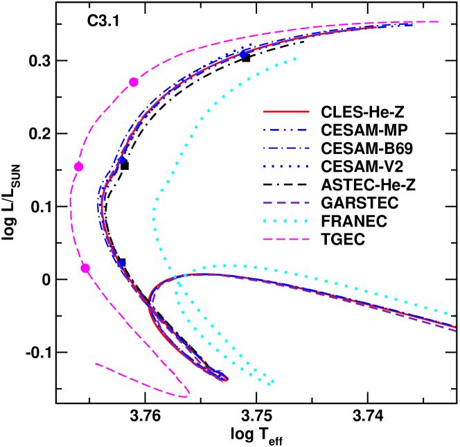
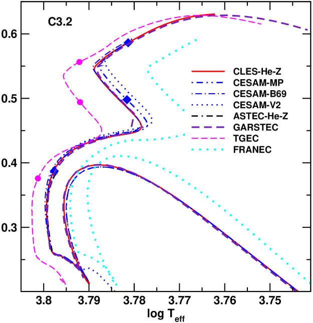
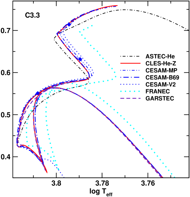
Figure 1: Evolutionary tracks and/or location of the target models A, B, C in the H–R diagram obtained for the 3 cases with the codes ASTEC-He (black, small dot-dash), ASTEC-He-Z (black, dash-dash-dot), CESAM-V1-MP (blue, dash-dot-dot), CESAM-V1-B69 (blue, large dot-dash), CESAM-V2 (blue, dots), CLÉS-He-Z (red, solid), FRANEC (cyan, dot), GARSTEC (indigo, small dash) and TGEC (magenta, large dash).

3 Models comparison

3.1 H–R diagram

Fig. 1 shows, for the different codes, the evolutionary tracks in the H–R diagram for the three cases considered and/or the location of the target models A, B, C. Note that all tracks have not been provided for each case and that in the case of ASTEC we chose to plot models including diffusion of helium and metals when available, rather than models including He diffusion only. Tracks obtained with the ASTEC-He-Z, CESAM-V1 (MP or B69), CLÉS and GARSTEC codes are very close. For these codes the differences in luminosity, radius and effective temperature generally remain well below 1 per cent except for Case 3.1B where the maximum difference in luminosity is close to 2 per cent. For the FRANEC and TGEC models and to a lesser extent CESAM-V2 models, differences with the other models amount to several per cents (with a maximum of about 25 per cents for Case 3.1C), that is at the same level or even larger than what we had found in Task 1 where the comparisons had covered a larger range of masses, chemical compositions and evolutionary stages but without diffusion. This could indicate that there remain small differences in the input physics of the CESAM-V2, TGEC and FRANEC models (opacities, equation of state, nuclear reaction rates, etc.) with respect to those specified for the comparisons. Although many efforts have been made in Task1 (see for instance Degl’Innocenti & Marconi [2005]), we have not yet fully traced their cause.

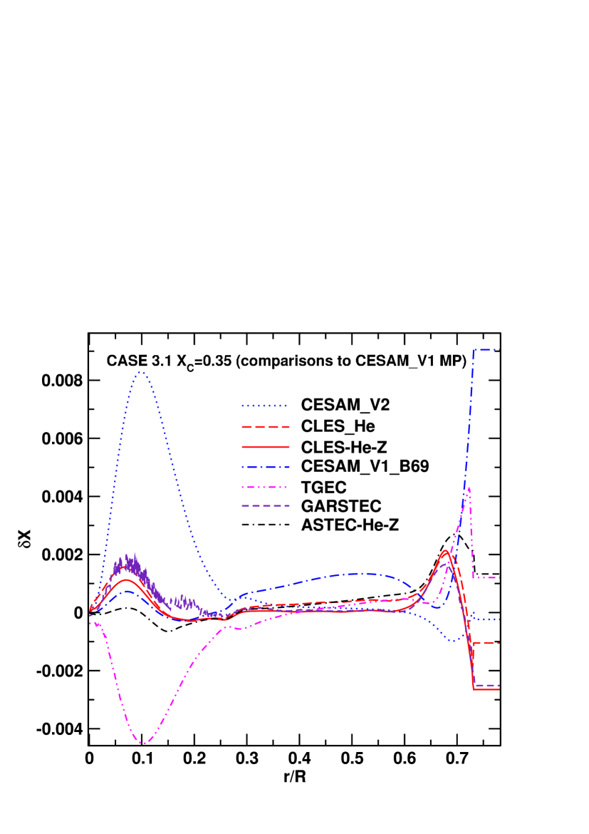
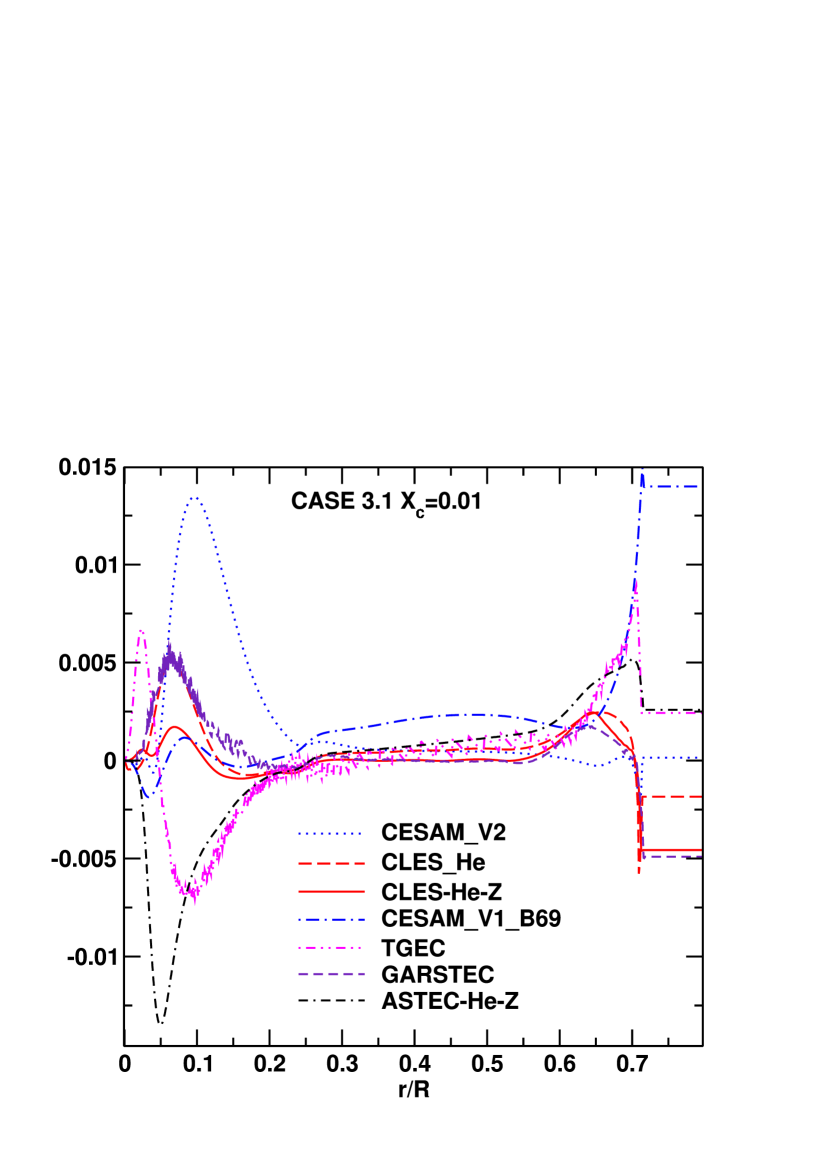
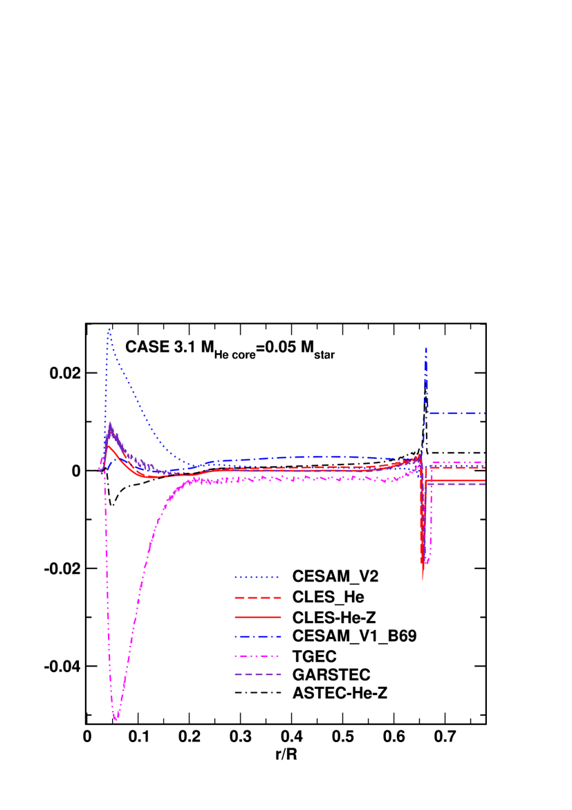
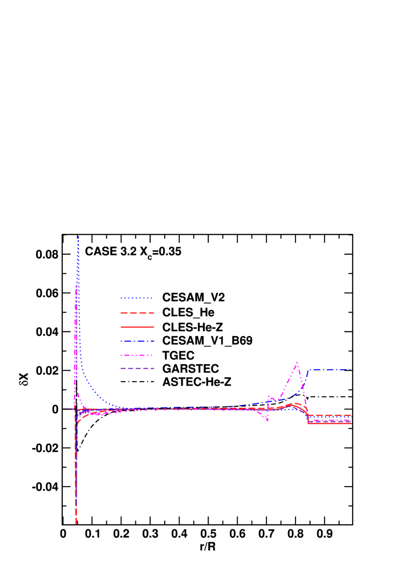
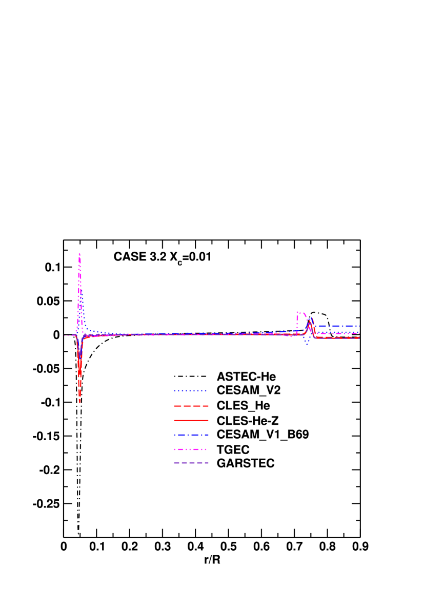
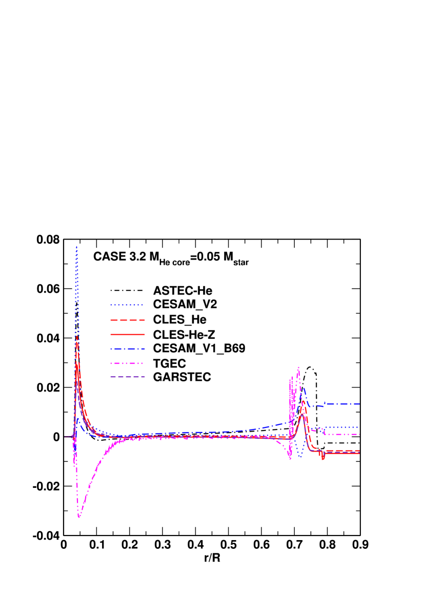
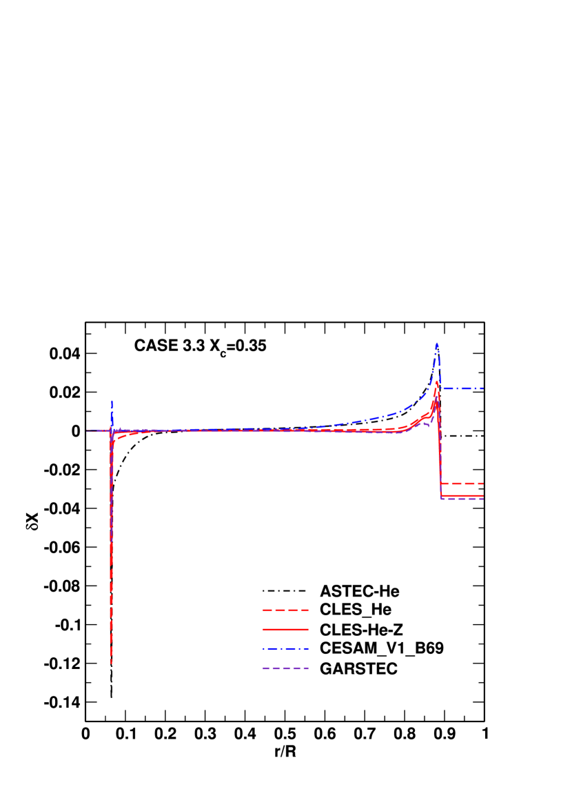
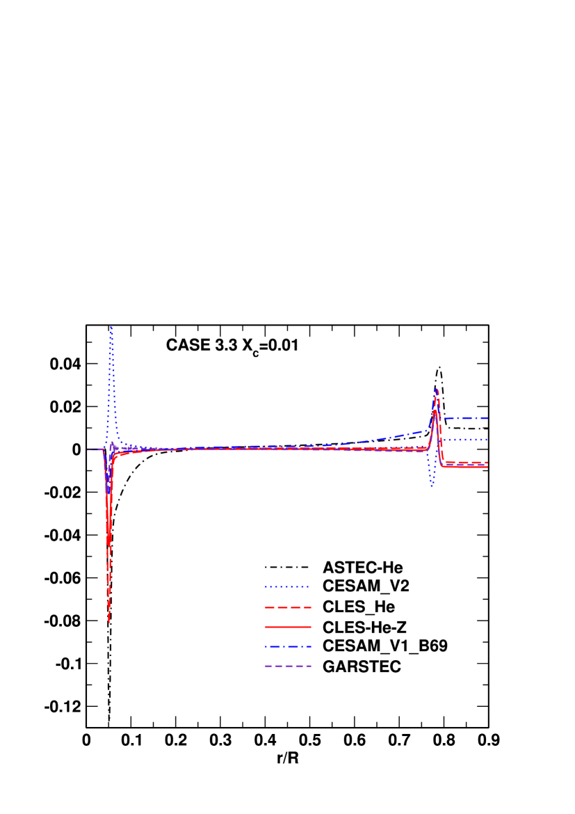
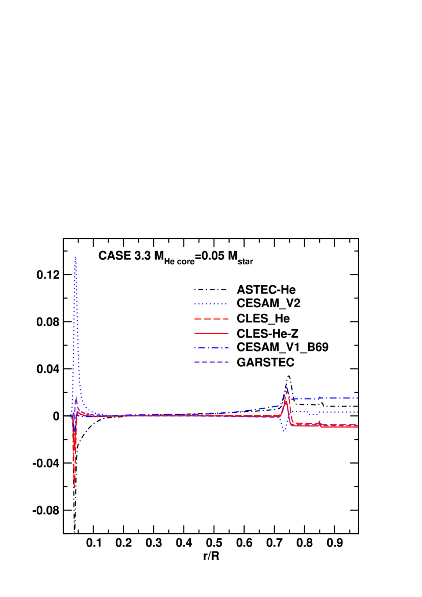
Figure 2: Lagrangian differences of the hydrogen abundance as a function of the normalised stellar radius between each model and the CESAM-V1-MP model corresponding to Case 3.1 (upper panel), Case 3.2 (middle) and Case 3.3 (lower panel) and phases A (left), B (centre) and C (right). The results of different codes or versions of a code have been considered: ASTEC-He (black, small dot-dash), ASTEC-He-Z (black, dash-dash-dot), CESAM-V1-B69 (blue, large dot-dash), CESAM-V2 (blue, dots), CLÉS-He (red, large dash), CLÉS-He-Z (red, solid line), GARSTEC (indigo, small dash), TGEC (magenta, dash-dot-dot).

3.2 Internal structure and surface abundances of the elements

Fig. 2 shows the Lagrangian difference $\delta X$ of the hydrogen abundance between each model and the CESAM-V1-MP model calculated at the same mass by means of the ADIPLS package tools and plotted as a function of the normalised radius for the 9 models selected (3 cases, 3 phases). Similarly, Figs. 3 and 4 show, respectively, the Lagrangian difference $\delta\ln c$ of the sound speed and $\delta\ln\Gamma_{1}$ of the adiabatic exponent between each model and the CESAM-V1-MP model. All models provided in the required GONG format have been represented (but see comparisons between FRANEC and CESAM in Marconi [2007]). Note that the scale on the vertical axis differs from one figure to the other.

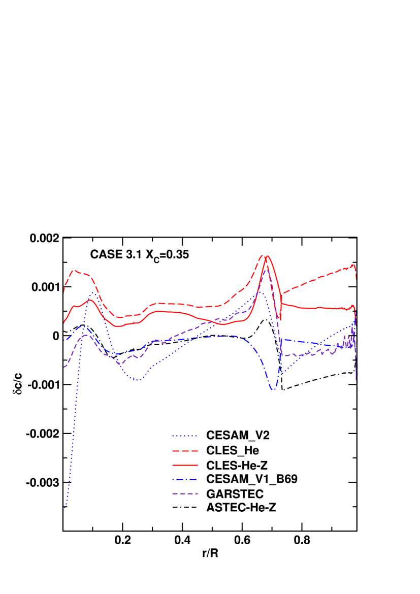
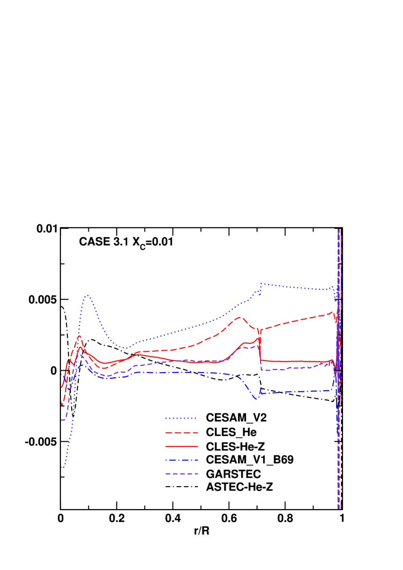
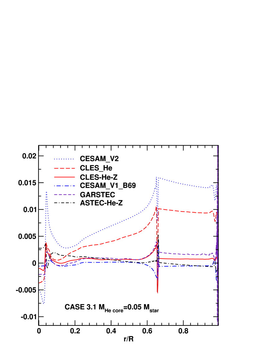
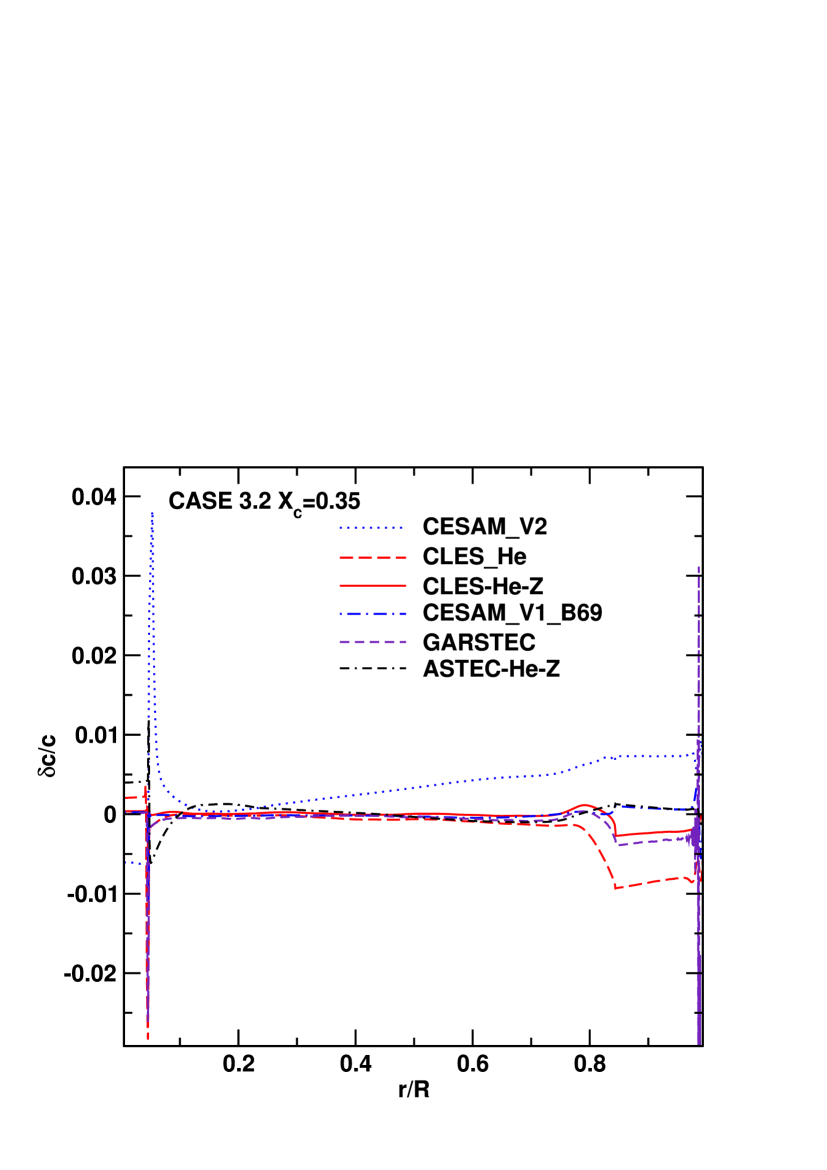
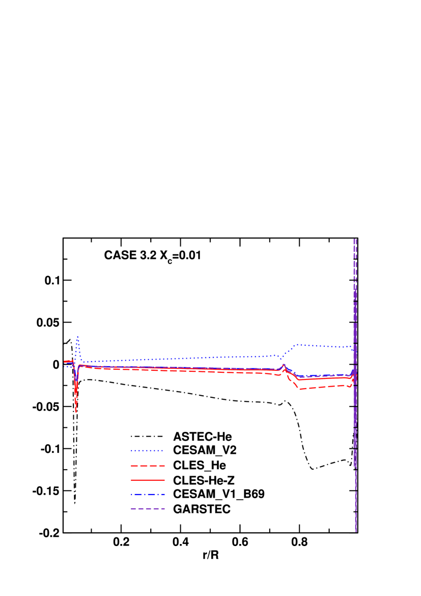
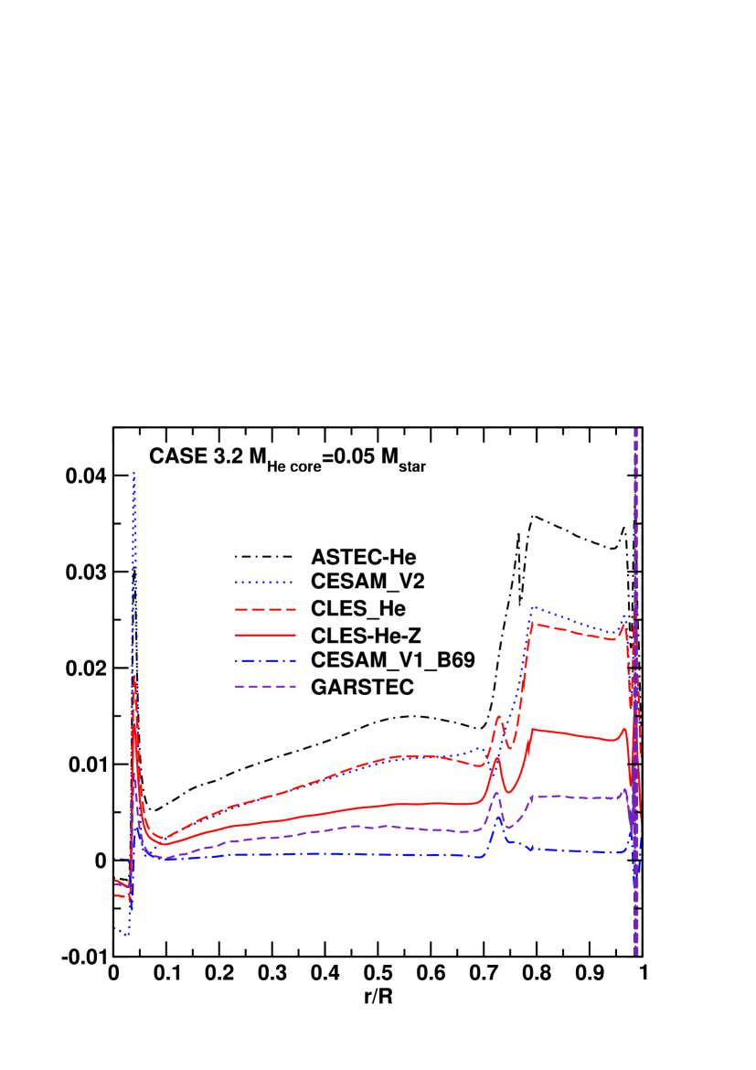
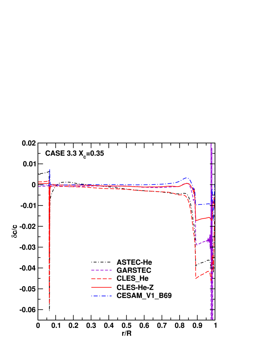
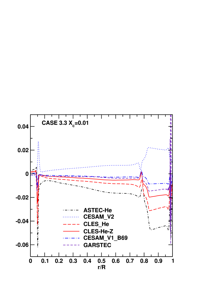
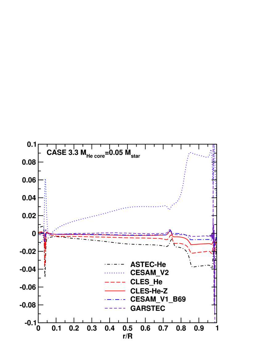
Figure 3: Same as in Fig. 2 but for the Lagrangian differences of the sound speed ($\delta\ln c$).

Concerning the hydrogen profile (Fig. 2), the major differences are located (1) at the frontier of and inside the convective envelope and, (2) in the central regions, i.e. in the region where $r/R_{\mathrm{star}}\lesssim 0.25$ for Case 3.1 and at the border of the convective core for Cases 3.2 and 3.3. Differences generally grow as the evolution proceeds from phase A to phase B and C and as mass increases. The differences found are, as expected, larger than those obtained in Task 1 where we compared (simpler) models with no diffusion. The larger differences are generally obtained for the CESAM-V2 and TGEC codes where some of the input physics probably do not follow exactly the specifications proposed for the comparisons. We also find rather marked differences of the ASTEC-He-Z and/or ASTEC-He models in the central regions mainly for phase B models for the 3 cases.

As discussed by Montalbàn et al. ([2007], hereafter MTL07), the differences in the sound speed in Fig. 3 reflect the differences (1) in the radius of the models, (2) in the chemical composition gradient in the envelope for $r>0.6\ R_{\mathrm{star}}$ and, (3) in the position of the boundaries of convection zones. The differences in the adiabatic exponent $\Gamma_{1}$ in the external regions of the model shown in Fig. 4 are related to the difference in the helium abundance in the convective envelope.

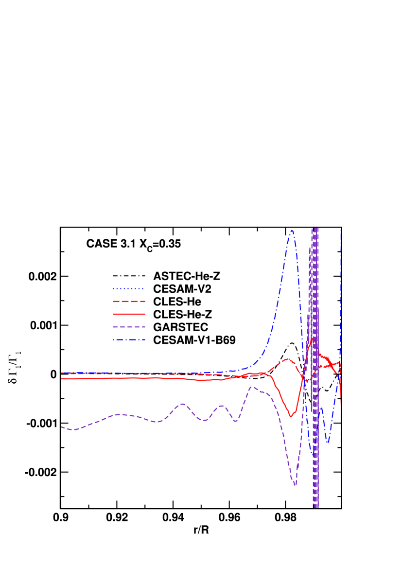
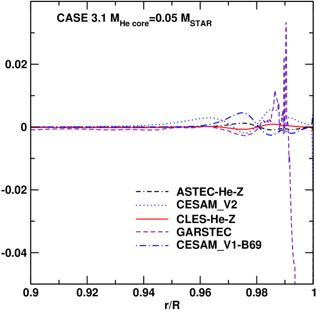
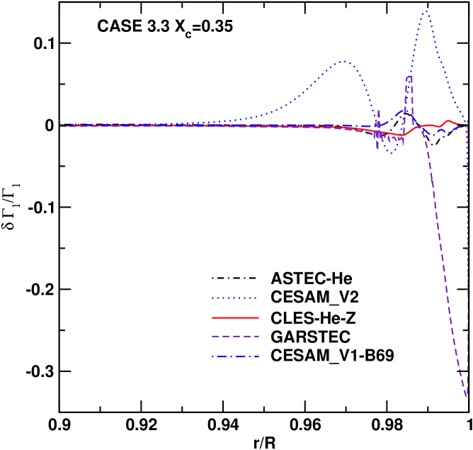
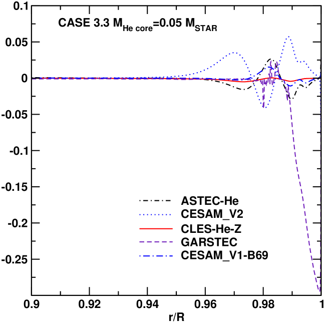
Figure 4: Lagrangian differences of the adiabatic exponent ($\delta\ln\Gamma_{1}$) as a function of the normalised stellar radius between each model and the CESAM-V1-MP model corresponding to Case 3.1 (upper panel) and Case 3.3 (lower panel) and phases A (left) and C (right). Different codes or versions of a code have been considered: ASTEC-He (black, small dot-dash), ASTEC-He-Z (black, dash-dash-dot), CESAM-V1-B69 (blue, large dot-dash), CESAM-V2 (blue, dots), CLÉS-He (red, large dash), CLÉS-He-Z (red, solid line), GARSTEC  (indigo, small dash).

The enhancement of the surface abundance of hydrogen and the concomitant depletion of helium and metals differ from one code to another. The surface abundance of He obtained by the different codes is displayed in Fig. 5, for each case and phase considered. The most important scatter is found for Case 3.1 where differences of the He surface abundance reach 0.07 in phases B and C if CESAM-V1-B69 models are excluded from the comparison and 0.19 if they are included. For Cases 3.2 and 3.3 the differences are lower: they are in the range 0.01-0.03 if CESAM-V1-B69 and FRANEC models are excluded and 0.02-0.08 if they are included. From Fig. 5, it is clear that in FRANEC models the depletion of the surface helium abundance has a tendency to be larger than in other models while it is always lower in CESAM-V1-B69 models than in other models.

Differences in the diffusion velocities may explain the differences in the surface abundances seen in Fig. 2 and 5 (see MTL07 for comparisons between CLÉS and CESAM). Furthermore, because of diffusion metals pile up beneath the convective envelope and the increase of the metal abundance induces an increase of opacity which may trigger convective instability. As discussed by MTL07, this occurs in Cases 3.2 and 3.3 where semiconvection takes place beneath the convective envelope. The evolution of the unstable layers then depends on the numerical treatment of the convective boundaries in the codes. MTL07 show that because of a different treatment of the convection borders, the CLÉS and CESAM codes produce external convective zones with different depths which in turn affects the surface abundances.

As discussed by MTL07, semiconvection can also take place at the border of the convective core in Cases 3.2 and 3.3. At the boundary of the convective core, nuclear burning builds a helium abundance gradient. In the diffusion equation, two terms are therefore in competition: the He gravitational settling term which makes helium travel towards the centre and the term due to the composition gradient which pushes helium outwards (Richard et al. [2001]). In Cases 3.2 and 3.3, when the second term becomes dominant, helium goes out of the core and so do the metals and this prevents settling. The increase of the metals at the border of the convective core makes the opacity increase and semiconvection appears. Again, the different numerical treatments of the convective boundaries in the codes can explain the differences seen in the models in the regions just above the convective core in Cases 3.2 and 3.3 (see Fig. 2).

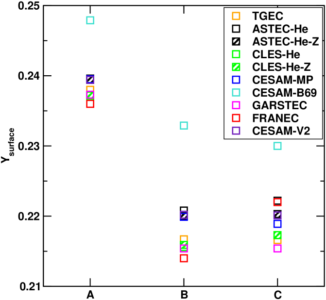
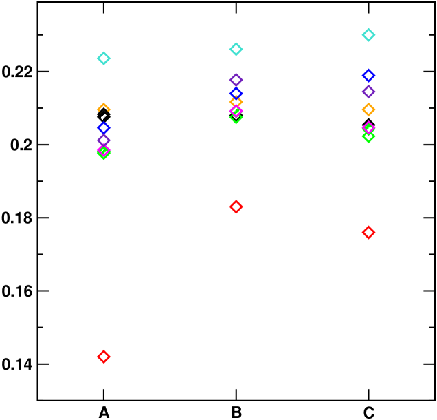
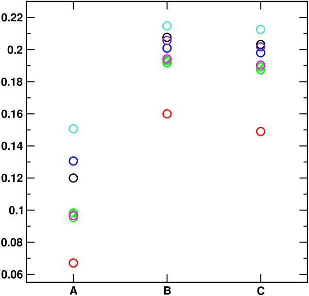
Figure 5: Surface abundance of helium in models computed by different evolution codes for Case 3.1 (squares, left), Case 3.2 (diamonds, middle) and Case 3.3 (circles, right) and phases A, B and C. The results of different codes or versions of a code have been considered: ASTEC-He (black), ASTEC-He-Z (black-hashed), CESAM-V1-MP (blue), CESAM-V1-B69 (cyan), CESAM-V2 (indigo), CLÉS-He (green), CLÉS-He-Z (green-hashed), FRANEC (red), GARSTEC (magenta), TGEC (orange).

4 Conclusion

In ESTA-Task 3 we have compared models of $1.0,1.2,1.3$ ${\mathrm{M}}_{\odot}$ on the M–S and subgiant branch which were computed with six different stellar evolution codes and different implementations of microscopic diffusion.

We found rather large differences in the H–R diagram and internal structure for the TGEC, FRANEC and to a lesser extent CESAM-V2 models. These differences are probably due to small remaining differences between the basic input physics of these codes and those specified for Task 1 and 3. We also find rather marked differences of the hydrogen abundance profile in the central regions for the ASTEC models in phase B models close to the end of the M–S.

Furthermore we showed that the surface depletion of helium due to diffusion is stronger in FRANEC models and much less strong in CESAM-V1-B69 models compared to the other models. The surface depletion of He is sensitive to the numerical treatment of the convective borders, particularly in presence of semiconvection just beneath the convective envelope and to the diffusion velocities. A further step in the comparison will consist in examining in detail the treatment of the convective boundaries in each code.

The differences between CESAM-V1-B69 models and others are presently not understood. For instance, CLÉS and CESAM use different diffusion velocities because CLÉS is based on the TBL94 formalism while CESAM uses Paquette et al. ([1986]) collisions integrals. Furthermore CESAM follows explicitly each element inside $Z$ and determines the ionisation degree of each species while some codes, like CLÉS adopt full ionisation and follow a reduced number of species. However, the consequences of these differences were carefully examined by MTL07, who showed that while the differences between CESAM-V1-MP and CLÉS models are rather well understood it is not the case for the differences between CESAM-V1-B69 and CLÉS models. To progress, it will be necessary to go deeper into the tests of the algorithm that solves Burgers’ equations in CESAM.