Kinematics of diffuse ionized gas in the disk halo interface of NGC 891 from Fabry-Pérot observations

Abstract

Context. The properties of the gas in halos of galaxies constrain global models of the interstellar medium. Kinematical information is of particular interest since it is a clue to the origin of the gas.

Aims. Here we report observations of the kinematics of the thick layer of the diffuse ionized gas in NGC 891 in order to determine the rotation curve of the halo gas.

Methods. We have obtained a Fabry-Pérot data cube in H$\alpha$ to measure the kinematics of the halo gas with angular resolution much higher than obtained from HI 21 cm observations. The data cube was obtained with the TAURUS II spectrograph at the WHT on La Palma. The velocity information of the diffuse ionized gas extracted from the data cube is compared to model distributions to constrain the distribution of the gas and in particular the halo rotation curve.

Results. The best fit model has a central attenuation $\tau_{{\rm H\alpha}}=6$, a dust scale length of 8.1 kpc, an ionized gas scale length of 5.0 kpc. Above the plane the rotation curve lags with a vertical gradient of -18.8 km s^-1 kpc^-1. We find that the scale length of the H$\alpha$ must be between 2.5 and 6.5 kpc. Furthermore we find evidence that the rotation curve above the plane rises less steeply than in the plane. This is all in agreement with the velocities measured in the HI.

1 Introduction

Over the last decade, diffuse ionized gas (DIG) in the halos of spiral galaxies has been identified as an important constituent of the interstellar medium (ISM). The detection of an extended layer of DIG in NGC 891 ($z_{{\rm NW}}$=0.5 kpc, $z_{{\rm SE}}$=0.3 kpc, Dettmar (1990)) , which was found to be similar to the extended layer of DIG, or Reynolds layer, (Reynolds, 1990) of the Milky way (Dettmar, 1990; Rand et al., 1990), was followed by several H$\alpha$ imaging searches. By now, many results on ‘normal’ (i.e., excluding nuclear starbursts) edge-on galaxies have been published (Dettmar, 1992; Rand et al., 1992; Pildis et al., 1994a; Rand, 1996; Rossa & Dettmar, 2003). Rossa & Dettmar (2003) cataloged 74 galaxies and found about 40% to have extraplanar diffuse ionized gas (eDIG). In those objects showing H$\alpha$ emission from the halo, a wide range of the spatial distributions have been found, from thick layers with filaments and bubbles (NGC 4631, NGC 5775) (Dettmar, 1990; Rand et al., 1990; Pildis et al., 1994b; Hoopes et al., 1999; Miller & Veilleux, 2003) to individual filaments and isolated plumes (e.g., UGC 12281)(Rossa & Dettmar, 2003). For only a few of them there is evidence for widespread DIG in the halo comparable to that in NGC 891. In this galaxy the DIG is distributed in long filaments and bubbles of ionized gas embedded in a smooth background.
     Since its emission line spectrum is rather easily accessible by optical imaging and spectroscopy, the DIG component is an important tracer of the ISM halo in other galaxies. This is true particularly since most other tracers, such as radio continuum from cosmic rays or X-rays from hot plasma, cannot be observed either with comparable angular resolution or with sufficient sensitivity.
     The origin and ionization source of the DIG component is still under debate and gives important constraints for models of the ISM in general and on the large-scale exchange of matter between disk and halo in particular (e.g., Dettmar, 1992; Rand, 1997).
     Theorists describe the disk-halo interaction by means of galactic fountains (Shapiro & Field, 1976; Bregman, 1980; de Avillez & Breitschwerdt, 2005), chimneys (Norman & Ikeuchi, 1989), and galactic winds (Breitschwerdt et al., 1991; Breitschwerdt & Schmutzler, 1999). Possible models trying to explain gaseous galaxy halos as a consequence of stellar feedback therefore depend on many factors, such as supernova rates, galaxy mass, magnetic fields and the vertical structure of the ISM.
     NGC 891 and NGC 4631 are two galaxies with extensively studied ISM halos. Both of them not only show prominent thick layers of DIG, they also have extended radio continuum, HI, and X-ray halos. The spatial correlation of radio continuum emission, indicative of cosmic rays in a magnetic field found in a thick disk, and extra-planar DIG has been discussed for NGC 891 in detail (Dettmar, 1992; Dahlem et al., 1994).
     If the DIG and other components of the ISM in the halo are due to dynamical processes, important information on its origin and ionization could come from kinematic studies. In the case of NGC 891 a first study was made by Keppel et al. (1991). Subsequent studies show that there is evidence for peculiar velocities of DIG. Pildis et al. (1994b) find a maximum difference with the HI rotation curve $\delta v_{{\rm max}}$=40 km s^-1; Rand (1997) retrieves a difference in the observed mean velocity of 30 km s^-1 between velocities at z=1 kpc and z=4.5 kpc. Also in the HI peculiar velocities are observed (Fraternali et al., 2005; Swaters et al., 1997). For both components, a deviation from corotation is observed on scales of 2 kpc above the disk in the sense that the gas rotates more slowly than expected. This “lagging” has been found to have a gradient of $dV_{{\rm rot}}/dz$=-15 km s^-1kpc^-1 in HI (Fraternali et al., 2005). Recent SPARSE-PAK observations (Heald et al., 2006) show a similar result for H$\alpha$.
      In order to understand this lagging, hydrostatic models have been investigated. These models are able to reproduce the lag of the halo of NGC 891 in HI (Barnabè et al., 2006). However, the stability of these models remains unresolved. A different approach to understanding the lag of halos are ballistic models (Collins et al., 2002; Fraternali & Binney, 2006). Fraternali & Binney (2006) are able to reproduce the vertical HI distributions of NGC 891 and NGC 2403 this way. However, their model fails in two important aspects: (1) they do not reproduce the right gradient in rotation velocity; (2) for NGC 2403 they predict a general outflow where an inflow is observed.
      It is clear that improved data on the detailed kinematics of the extra-planar DIG would be very useful to a further physical understanding of the phenomenon.
     Here we present a full velocity cube for the DIG in NGC 891 from observations with the TAURUS II imaging Fabry-Pérot spectrograph. As a byproduct, we obtain a very clean map of the H$\alpha$ distribution. NGC 891 has a systemic velocity of 528 km s^-1 (RC3) and we assume a distance of 9.5 Mpc (van der Kruit & Searle, 1981). At this distance 1 arcmin corresponds to 2.8 kpc physical size. We present the observations in $\S$ 2 and the data reduction steps in $\S$ 3. $\S$ 4 will show the results that can be obtained by rebinning the data. In $\S$ 5 we will present models for the gas distribution and these models will be discussed and compared to the data in $\S$ 6. We will summarize and conclude in $\S$ 7.

2 Observations

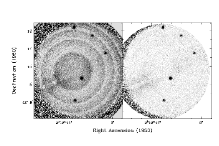
Figure 1: This channel of original wavelength calibrated data cube at v=674 km s^-1 demonstrates the contamination by night sky lines with varying intensity (left). The effect of removing a model for the night sky contribution from averaging in rings is seen on the right.

Figure 2: Model for the night sky contribution obtained by averaging in rings as used for the channel shown in Fig. 1.

The data were obtained during two nights in November 1992 with the TAURUS II imaging Fabry-Pérot spectrograph at the William-Herschel Telescope on La Palma. The attached EEV3 CCD detector with a pixel size of 22.5 $\mu$m provided an image scale of 1.”04/pixel with a binning by 2. An interference filter with central wavelength at $\lambda=$657.7 nm and a bandpass of 1.5 nm was used for order separation. The field of view was restricted to 5.6’$\times$5.6’ due to blocking by the prefilter. Two slightly overlapping fields in NGC 891 were therefore observed to cover the inner $\sim$ 10’. The North-East field was located at RA$=2^{h}22^{m}36.8^{s}$, DEC$=42^{\circ}22^{\prime}32.2"$ (J2000) and the South-West field at RA$=2^{h}22^{m}26.7^{s}$, DEC$=42^{\circ}18^{\prime}5.8"$ (J2000). The observations were taken under non-photometric conditions, with poor seeing of typically 2 arcsec. For object exposures 75 etalon steps, with a step size of $\Delta\lambda=$0.02742 nm, were used with an integration time of 70 s each. Full data cubes were taken at the beginning of each night with a flat field lamp, and during the night several cubes were taken using the CuNe lamp to allow us to determine the wavelength dependence in each channel.

Date	Run-No:	Field	UT/Start	Airmass/Start
Nov 16/17 1992	3559	NE	19:29	1.03
	3564	SW	00:44	1.05
Nov 17/18 1992	3581	NE	21:46	1.04
	3583	NE	01:09	1.10

Table 1: Log of the observations

3 Data Reduction

A slight gradient in the bias level of 1 ADU across the field was removed in all data cubes because at the amplifier setting this accounted for a 10$\sigma$ signal with respect to the read-out noise. The IRAF package was used for these first data-processing steps including flatfielding and cosmic-ray filtering. For all further processing steps we made use of the GIPSY package, which is better suited for these kinds of data cubes.
     Cuts in the velocity direction averaged over areas of the night sky showed significant variations from channel to channel, up to 20% in the night sky contribution with a systemic jigsaw pattern. This pattern is due to the stepping pattern used for scanning over the $\sim$ 2 hrs of observation for each on-source cube. Significant brightness changes of two bright night sky lines were not correlated to these changes in the sky background. We corrected for the variations of the night sky brightness by subtracting a constant determined for each channel.
     The phase calibration was obtained by fitting a model to the scans of the CuNe lamp; this way the step size was determined to be 0.02748 nm. Rebinning the object data cubes with the appropriate model resulted in four complete data cubes on the object, three for the field in the North-East and one for that in the South-West.
     The rebinned images still contained the night sky lines. The strong OH night sky lines at $\lambda=6568.78$ $\AA$ and $\lambda=6577.28$ $\AA$ were used to establish the absolute wavelength calibration. They also provide a check on the channel step size. The $\Delta\lambda=$0.02742 nm determined this way is in excellent agreement with the determination from the afore-mentioned calibration cube and corresponds to 12.5 km s^-1 at H$\alpha$ (for Fabry-Pérot data reduction techniques see Bland & Tully (1989); Jones et al. (2002)). The profile of the night sky lines also provides information on the spectral resolution, which was determined to be 40.7 km s^-1(FWHM). The formal errors of the Gaussian fits to the OH-night sky lines allowed us to estimate the error of the wavelength scale to be less than 6 km s^-1. A correction to the observed velocity of -4.2 km s^-1 was needed to obtain the heliocentric velocity.
     At this stage, one remaining problem was caused by the redistribution of the varying line intensity of the night sky lines during the integration of the observed cube into a wavelength cube. Rebinning of the lines into the appropriate wavelength channels resulted in a strong pattern of rings. In the left-hand panel of Fig. 1, we show this effect for the worst case. To overcome this artifact for all affected channels the rings of the line emission were cut out interactively in areas well separated from the galaxy by using the GIPSY routine BLOT. The result was integrated using the routine ELLINT using the center as determined from the phase calibration and the mean value in individual rings was used as a model. Such a ring model is given in Fig. 2. The subtraction of the model resulted in general in a satisfactory reduction of the artifact as demonstrated in the right hand panel of Fig. 1. Typically, the resulting residuals are smaller than the noise level of the night sky. This can be judged from the right panel in Fig. 1. However, some of the channels showed residual larger than the noise level of the night sky. These residual rings were masked manually.
     These cleaned and wavelength-calibrated data cubes covered a velocity range of 940 km s^-1, sufficiently large to provide us with a scaled sum of continuum channels to correct for the continuum. This continuum correction also removed all ghost images from internal reflections of the instrument.
      We flux calibrated the observations by comparing 7 HII regions in the integrated velocity map with the calibrated H$\alpha$ image from Heald et al. (2006). 4 of these regions were located in the NE pointing and 3 in SW pointing. We estimate the uncertainty of this calibration to be $\sim$ 10%.
     For the merging of all data and for comparison with other data sets, in particular the HI map provided by Fraternali et al. (2005), astrometry was performed. Since the two fields do not sufficiently overlap, we used five stars with positions obtained from DSS to re-grid the two fields into a common map. The astrometric accuracy from the fits to the stars is $\sim$ 2 arcsec. Finally the data cubes were combined into one cube, rotated by 42 degrees in position angle to be oriented along the major axis and cut back to 42 channels to cover the velocity spread in NGC 891. The noise in a channel in the fully reduced and calibrated cube is 1.2$\times 10^{-18}$ erg s^-1 cm^-2 arcsec^-2 in the NE pointing and 1.4$\times 10^{-18}$ erg s^-1 cm^-2 arcsec^-2 in the SW.

4 Results

For the following analysis, in order to obtain a better S/N, the data were binned. In order maintain resolution in higher emission parts, this was done in such a way that the length and width of a bin increases exponentially as the distance to the major and minor axis increases. For the North-East side of the galaxy no binning was applied when the S/N in a pixel was $\geq$ 4. The channel at the systemic velocity ($v_{{\rm sys}}=528$ km s^-1) was set to 0 km s^-1 and all velocities given are offsets from this channel. The central position was determined by eye in several Palomar Sky Survey and 2MASS images to be RA$=2^{h}22^{m}33.0^{s}$, DEC$=42^{\circ}20^{\prime}51.5"$ and set to 0 in the images. From the scatter of the central position in the different bands we determine the error to be less than 2 arcsec. Notice that this value differs from the best determined position given by the NASA Extra-galactic Database by almost 6 arcsec in declination.
     For display purposes the figures shown in this paper come from a cube which was masked so that only regions with signal are shown. The mask was constructed by smoothing the original binned cube with a Gaussian of 4 arcsec FWHM, which was cut at the 1$\sigma$ level.

4.1 Channel maps

In Figs. 3 and 4 we give the resulting channel maps of H$\alpha$ emission with a velocity step size of $\Delta$v=12.5 km s^-1. In the following figures, the NE part of the galaxy is to the left; this is also the approaching side of the galaxy. Data are missing in small wedges along the minor axis, as we had underestimated the vignetting of the field when the required overlap of the fields was determined. It is noteworthy that a thick component in the H$\alpha$ emission is already visible in individual channel maps. This sudden thickening of the H$\alpha$-emitting gas layer was reported before from H$\alpha$ imaging (Rand et al., 1990; Dettmar, 1990; Pildis et al., 1994b). The channel maps also clearly show a dichotomy between the NE and SW part of the galaxy with regard to the overall intensity level of the H$\alpha$ emission.This was already noted by Rand et al. (1990) and can be seen most clearly in the spectacular color image of NGC 891 obtained by Howk & Savage (1997) (their Fig. 1) which shows a line of blue knots all along the north side at $|{\rm z}|=0$, and no such features on the south side. This dichotomy is also seen in the distribution of the non-thermal radio continuum emission. (Hummel et al., 1991)

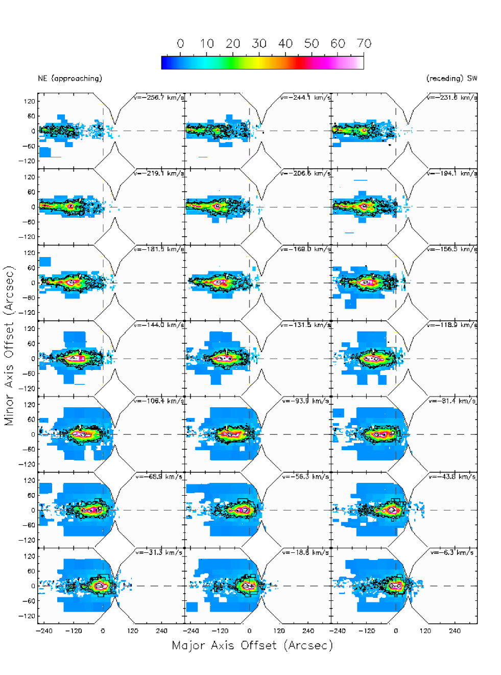
Figure 3: The velocity channel maps of the approaching side for the binned H$\alpha$ of NGC 891. The contours are at 25.3, 51, 510 $\times 10^{-19}$ erg s^-1 cm^-2 arcsec^-2. The horizontal and vertical dashed lines indicate the major and minor axis respectively.

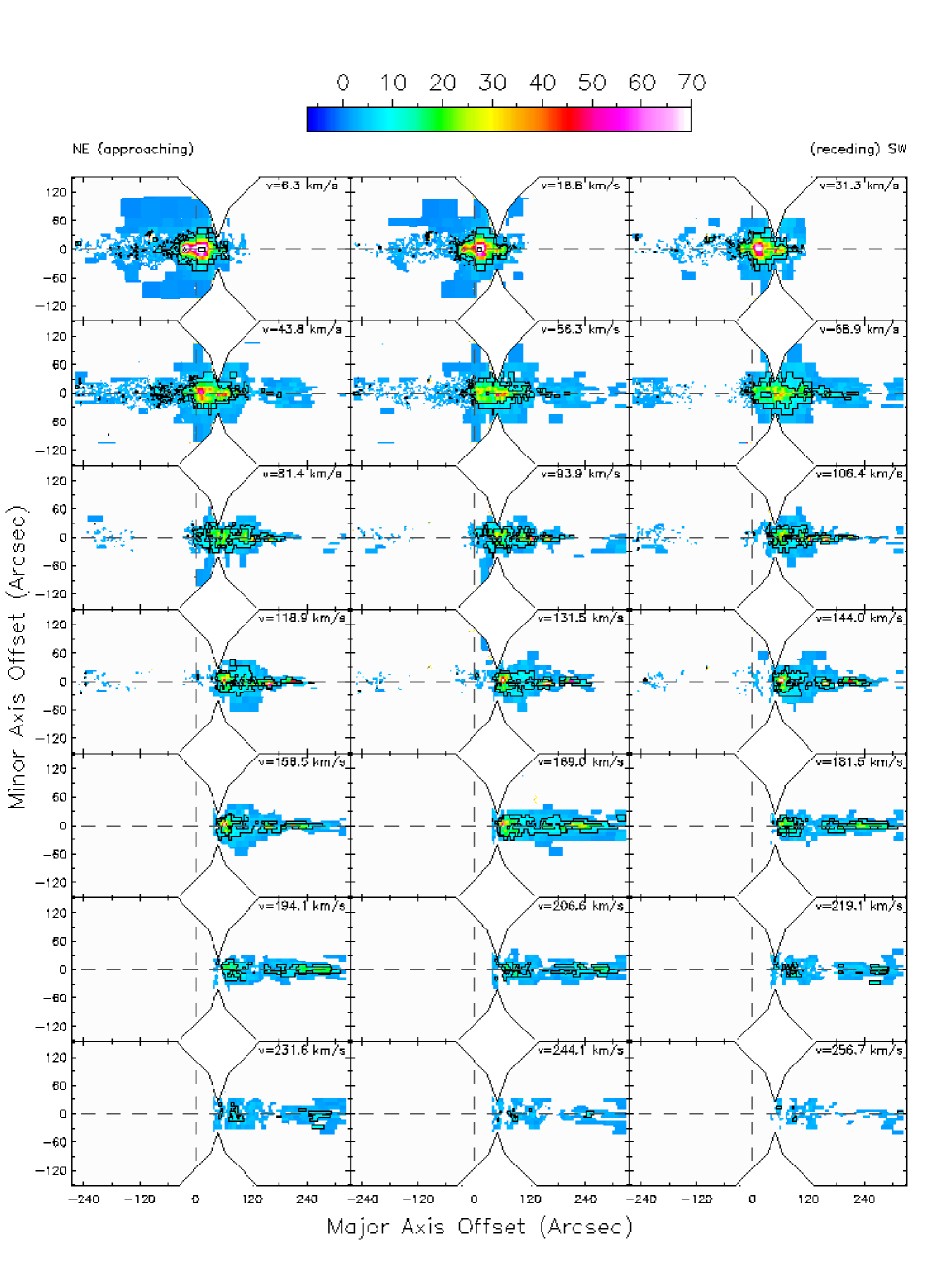
Figure 4: Same as fig. 3, for the receding side.

4.2 H$\alpha$ distribution

The dichotomy discussed in $\S$ 4.1 is seen even better in the total H$\alpha$ distribution, which is shown in Figure 6. This image was obtained by integrating all channel maps along the velocity axis of the cube. It clearly shows that the diffuse ionized gas (DIG) extends beyond our field of view in several places. On the NE side of the galaxy our whole image is filled with low-level emission; on the SW side, however, we are not able to distinguish more than the major axis of the galaxy. This suggests that the difference in intensity is a physical effect and not a line-of-sight effect (see further discussion $\S$ 6.2). For comparison we added a $F$-band image from the POSS II, below the H$\alpha$ image.

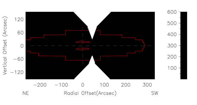
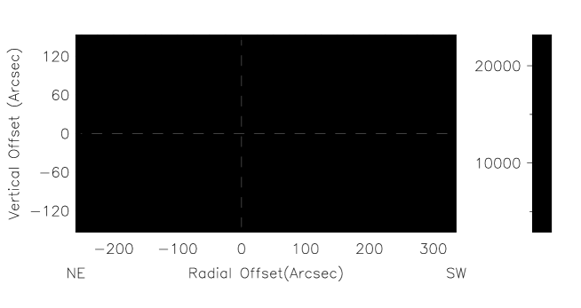
Figure 5: H$\alpha$ distribution from NGC 891 as obtained from integrating the binned channel maps. The black contours are at 1.0 and 10.0 $\times 10^{-17}$ erg s^-1 cm^-2 arcsec^-2. Red contours are the best fit model (see $\S$ 5.3) The horizontal and vertical dashed lines indicate the major and minor axis respectively.

Figure 6: $R$-band image taken from the Palomar Sky Survey for comparison with the H$\alpha$ distribution.The horizontal and vertical dashed lines indicate the major and minor axis respectively.

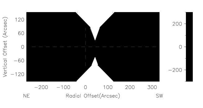
Figure 7: The velocity field of the observed H$\alpha$ determined by a Gaussian fitting to the line profiles. The contours are at -200, -100, 0, 100, 200 km s^-1 and are with respect to the systemic velocity of 528 km s^-1. The horizontal and vertical dashed lines indicate the major and minor axis respectively.

4.3 Velocity field

Fig. 7 shows the velocity field of our H$\alpha$ cube. This velocity field is determined by fitting a Gaussian profile to the line profile in each bin, the peak of this Gaussian is considered to be the velocity in this bin. This way we do not measure the real rotational velocity but an apparent mean velocity which is determined by a combination of the rotational velocity, the density distribution of the gas, and the opacity of the dust. This velocity will be referred to as the mean velocity. We chose the Gaussian fit because in the places where the underestimation of the rotational velocity is most significant (major axis, center of the galaxy) the H$\alpha$ is optically thick (see discussion).
     On the NE side we see a regular velocity field which resembles solid body rotation with some lower velocities in the bins at $|{\rm z}|=60$ arcsec. This would indicate that the H$\alpha$ lagging does not begin below 60 arcsec (2.8 kpc). However, as the optical depth declines we expect to look deeper into the galaxy. This would mean that we are receiving more emission from the line of nodes the further we are from the plane of the galaxy. Since the real rotational velocity should be determined at the line of nodes our underestimate of the velocity would be less the further we look into the galaxy. So for a cylinder with a declining optical depth in the $|{\rm z}|$-direction and solid body rotation we would expect the mean velocities to rise as the distance from the major axis increases. This is not the case for NGC 891 as we can see in Fig. 7.
     If we look at Fig. 7 and follow the -200 km s^-1 contour we see that, starting from major axis, the mean velocity first rises until $\sim 20$ arcsec above the plane. Then the mean velocity starts to drop up to $\sim 60$ arcsec. Above this the mean velocity starts to rise again but it is unclear whether this is real or a combined effect of the binning and Gaussian fit.
      Looking at the South-West side of the velocity field we see that this side is much more irregular in velocity than the North-East side. Following the 100 km s^-1 contour we see a behavior similar to that of the -200 km s^-1 contour only much more extreme. Since on the SW side above $\sim 60$ arcsec there is no emission it is unclear if the mean velocity would start to rise again above this height.

5 Models

5.1 Position - Velocity diagrams

An examination of ‘Position - Velocity diagrams’ (PV diagrams) provides the basis for our discussion of the H$\alpha$. These diagrams are another representation of the channel map data from Figs. 3 and 4, where now the profiles are extracted at each point along a locus of positions in the image of the galaxy and plotted as contours in the PV plane. Figure 8 is one example of this representation; here the position (x-axis) is measured along the major axis of the galaxy through the nominal center at $|{\rm z}|=0$, and on the y-axis radial velocity is given. The color scale represents the H$\alpha$ surface brightness observed at each position; for instance, the H$\alpha$ line profile at the position located 1 arcmin to the North of the galaxy center would be a line parallel to the velocity axis at a radial offset of -1 arcmin. In the following discussion we will concentrate on the NE side of the galaxy and refer to the absolute velocities.

5.2 PV-model

Parameters	Upper limit	Lower limit	Best fit model
Name	Model 1.1/M 1.2	Model 2.1/M 2.2	Model 3/M G3
$h_{\rm g}$ (kpc)	$6.5/5.5$	3.0/2.5	5.0
$z_{\rm g}$ (kpc)	0.8/0.8	0.8/0.8	0.8
$h_{\rm d}$ (kpc)	8.1/8.1	8.1/8.1	8.1
$z_{\rm d}$ (kpc)	0.26/0.26	0.26/0.26	0.26
$\tau_{{\rm H\alpha}}$	4-6/6	12-14/13-14	6
$\sigma_{\rm v}$ (km s-1)	40/40	40/40	40
$R_{\rm max}$	21/14	21/14	14

Table 2: Model parameters. The addition G to a model indicates that the rotation curve has a gradient of -18.8 km s^-1 kpc^-1 in the vertical direction. For the upper and lower limit there are two models which differ in truncation radius (See $\S$ 5.2 ). $h_{\rm g}$ and $z_{\rm g}$ are the scale length and height of the gas respectively. $R_{\rm max}$ is the truncation radius of the models.

The position velocity model is a FORTRAN code which calculates emission at every position of an exponential disk taking line of sight velocities into account. For every position the light is extincted as expected from a dust disk with a given optical depth and an exponential distribution with variable scale length and height. The structural parameters are defined in the same way as in the models used by Xilouris et al. (1998). If the radius of the disk exceeds a certain cut off ($R_{\rm max}$) all emission and absorption is set to 0. This is done to simulate a truncation radius. The code then integrates these values along the line of sight at every position and determines an observed velocity distribution and a intensity. Scattering is ignored in the calculations.
     The code allows the disk to be inclined and for NGC 891 we chose an inclination of 89^∘. To make a fit we assumed the HI rotation curve (Fraternali et al., 2005) and a truncation radius $R_{\rm max}=21$ kpc (van der Kruit & Searle, 1981). We fit the NE (left) side of the PV-diagram by eye. The SW (right) side is not taken into account because the signal is very irregular on this side (see $\S$ 4.3). We started with fitting some simple models where the scale length of the dust equals the scale length of the gas ($h_{\rm g}=h_{\rm d}=5$ kpc).
     These simple models all show a major discrepancy with the data at high velocities and large radii, where the intensities in the models start to rise again while in the data no such rise is seen. To solve this problem we needed the scale length of the dust to be longer than the scale length of the gas. Therefore we assumed that the dust disk has a scale length of 8.1 kpc (Xilouris et al., 1998).
      With this longer scale length for the dust the intensity peak at large radii and high velocities has disappeared and the general shape of the PV-diagram is now comparable to the data. Also it provides us with an upper limit for the scale length of the gas. At a gas scale length of 6.5 kpc (Model 1.1, see Table 2, Fig. 8 black contours) the problem of the simple model arises again. This is seen in Fig. 8 around -200 arcsec and -200 km s^-1 offset (pointed out by the black arrow) where the highest black contour of $48\sigma$ reappears while in the data no such thing is seen. Therefore we consider Model 1.1 as a upper limit for the gas scalelength. A lower limit for the scale length is found at 3.0 kpc (Model 2.1, see Table 2, Fig. 8 red contours). At this scale length we clearly see the second highest contour bending up around an offset of -200 arcsec and -200 km s^-1 (pointed out by the black arrow) while the same contour for the data continues almost up to the edge of the image at an offset of -230 arcsec and -225 km s^-1. Figure 8 also shows that we are overestimating the intensities at low velocities. To fit the low velocities at large radii a shorter truncation radius is needed in the models. Unfortunately this truncation radius is clearly outside our field of view. Thus we can only find the right truncation by fitting the PV-diagram. We find that a truncation at 14 kpc (${\rm R_{max}}$) fits the data the best. This differs from the radius of the optical truncation (${\rm R_{max}}$) determined by van der Kruit & Searle (1981) who obtain ${\rm R_{max}}$= 450 arcsec (21 kpc) but is in agreement with Rand et al. (1990) who find diffuse emission out to 15 kpc. When we determine the upper and lower limit on the scale length for models with a the new truncation radius for the ionized gas (14 kpc) (Model 1.2 and Model 2.2, see Table 2)we find that these models show the same behavior as Model 1.1 and Model 2.2 but at shorter scale lengths. This is caused by the fact that in the models not only the gas disk is now truncated at 14 kpc but the dust disk as well. It remains unknown which truncation is more suitable for the dust disk.

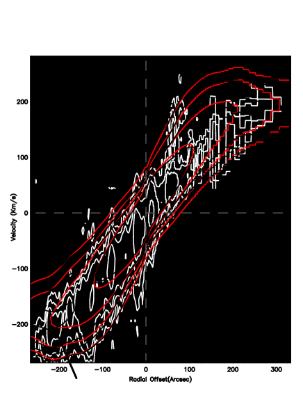
Figure 8: Color plot of the H$\alpha$ PV-diagram along the major axis overlaid with contours of Model 1 and 2 (see Table 2) corresponding to the upper and lower limit which can be fitted. White contours are the data at 3$\sigma$, 6$\sigma$, 12$\sigma$ and 48$\sigma$. Black contours are Model 1.1 with $\tau_{\rm H\alpha}=5$, red contours are Model 2.1 with $\tau_{\rm H\alpha}=13$. The black arrow indicates the place where the fits deviate from the data (see text).

Koopmann et al. (2006) recently found that on average the H$\alpha$ scale length for a field galaxy is on average 14 % longer than the stellar scale length. Based upon the value found by Xilouris et al. (1998) in the $V$-band this would mean that the deprojected H$\alpha$ scale length for NGC 891 should be $\sim$ 6.5 kpc which is in agreement with our limits.
     Although the central attenuation for a given scale length is quite well constrained, the differences in dust attenuation can be quite large between the different scale lengths. This gives us another handle on which scale length is correct. Xilouris et al. (1998) found a central optical depth of $\tau_{\rm face-on}=0.7\pm 0.01$ in $V$-band, for the galaxy seen face on. For our models for this edge-on galaxy this would translate to a central attenuation of $\tau_{\rm H\alpha}=10.9$. $\tau_{\rm H\alpha}$ in our models is the optical depth at a radial and vertical offset of 0 along the line of sight to the center of the disk.
We consider the model with $h_{\rm d}=5.0$ kpc, $\tau_{\rm H\alpha}=6$ and $R_{\rm max}$=14 kpc (Model 3) the best fit. Fig. 9 is an example of the major axis PV diagram of the data overlaid with contours of Model 3. Given the dependence of the central optical depth on scale length our results are not in disagreement with Xilouris et al. (1998).

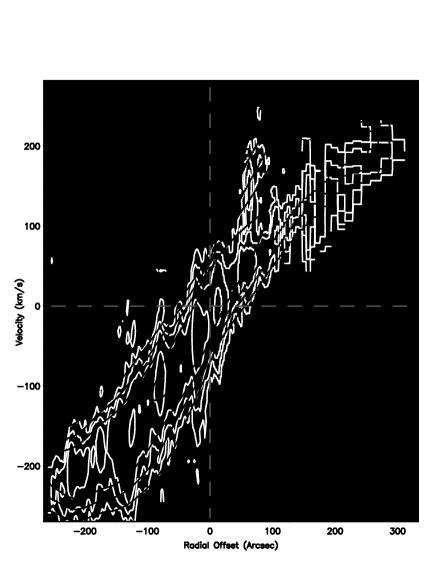
Figure 9: Color plot of the H$\alpha$ PV-diagram along the major axis overlaid with the contours of the best fit model.White contours are the data at 3$\sigma$ 6$\sigma$ 12$\sigma$ 48$\sigma$. Black solid contours are Model 3 (Table 2).

5.3 Image-model

After we fitted the PV-diagram on the major axis we put the same values into a FORTRAN code which calculates an intensity along the line of sight (see $\S$ 5.1). This code produces a model image which we can compare with the observed images of NGC 891. To determine the correct scale height we compare an intensity cut parallel to the minor axis averaged between -100 to -50 arcsec of the model images to the observed H$\alpha$ distribution averaged over the same region (Fig. 6). Since at this point we are interested only in the vertical shape above the dust, the maps are first normalized to their emission 30 arcsec above the plane. To determine the best fit we concentrate on the emission at a positive offset of the plane since this side is brightest. In our fit we only consider the emission at offsets larger than 30 arcsec. From this comparison we find that a scale height of 0.8 kpc best fits the data. We then determine from this comparison a scaling for the model so that it represents the unnormalized data. Figure 10 (left) shows this averaged cut along the minor axis. This figure shows the data (solid line) and the scaled model for $z_{\rm g}$=0.7 (dashed red line), 0.8 (dashed blue line), 0.9 (dashed green line) kpc. We see that $z_{\rm g}$=0.8 kpc is the best fit to the data.
      As a check on our scaling factor and our scale lengths Fig. 10 shows on the right a cut parallel to the major axis at a vertical offset of 30 arcsec. The solid black line is the data and the colored lines are the scaled models with a changing scale length with $h_{\rm g}$=3.0 kpc (dashed red line), $h_{\rm g}$=5.0 kpc (dashed blue line) and $h_{\rm g}$=6.5 kpc (dashed green line). This figure shows clearly that a scale length of 5 kpc is the best fit to the data.

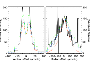
Figure 10: Normalized intensity cuts of integrated maps. Left: along the minor axis. H$\alpha$ (solid line)), $z_{\rm g}$=0.7 kpc (dashed red line), $z_{\rm g}$=0.8 kpc (dashed blue line), $z_{\rm g}$=0.9 kpc (dashed green line). Right: Parallel to the major axis at a vertical offset of 30 arcsec. H$\alpha$ (solid line)), $h_{\rm g}$=3.0 kpc (dashed red line), $h_{\rm g}$=5.0 kpc (dashed blue line), $h_{\rm g}$=6.5 kpc (dashed green line)

5.4 Cube model

Having obtained the best fits for the images and the major axis PV-diagram we model a full data cube so we can obtain PV-diagrams at any height in the disk. We constructed two of these cubes based on the the best fit of the major axis PV-diagram. These cubes are then binned in the same way as the data and scaled with the previously derived scaling factor. In one of these cubes the rotation curve is kept constant throughout the vertical distribution of the cube (Model 3, see Table 2). The other cube model contains a vertical gradient for the rotation curve of -18.35 km s^-1 kpc^-1 (Model G3, see Table 2). In this model the radial shape of the rotation curve is not changed. These cubes and their comparison to the data will be presented below.

6 Discussion

6.1 Kinematics in the plane

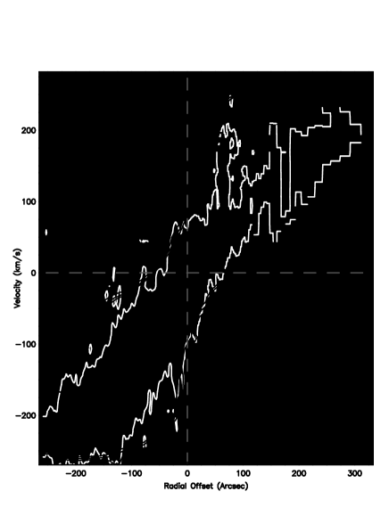
Figure 11: Color plot of the H$\alpha$ PV diagram along the major axis. For comparison the HI PV diagram on the major axis is over plotted at contour levels 3$\sigma$, 6$\sigma$ and 9$\sigma$.

Figure 11 shows a PV diagram of the H$\alpha$ emission along the major axis of the galaxy ($|z|=0$). This diagram bears the signature of solid body rotation instead of showing the strong differential rotation of the HI. The simplest interpretation of this is that the disk of the galaxy is optically thick at $|z|=0$, so that the H$\alpha$ emission we see is mostly coming from the front edge of the disk. This is consistent with $\tau_{\rm H\alpha}$=6.

Figure 12: Normalized velocity line profiles of the H$\alpha$ (Solid line) and HI(dashed line)on the major axis at a radial offset of -1 arcmin. The straight lines indicate the 3 $\sigma$ values for both observations

Let us consider one ‘cut’ through this diagram parallel to the velocity axis, at a radial offset of -1 arcmin (Fig. 12). Presuming that the H$\alpha$ emission emanates from gas which is in circular rotation, the H$\alpha$ emission at $|25|$ km s^-1 is at the very front of the disk. There is an absence of emission at lower velocities because the H$\alpha$ disappears as we get to the front edge of the disk of the galaxy. As we descend in this diagram towards $|175|$ km s^-1, at the same radial offset, the emission fades out. We interpret this as a result of increasing extinction due to dust in the plane. From our best fit model, approximately 6.5 magnitudes of extinction, along the line of sight to the center of the galaxy, are implied by this interpretation of the data; assuming that there is no extinction in the HI.
      As we sample H$\alpha$ emission at larger radial offset we look closer to the line of nodes, and the velocities increase until we actually look at the line of nodes and the velocities do not rise anymore. Note though that due to the clumpiness of the emission sources the velocities can still decrease after this point.
     Alternatively, the H$\alpha$ emission may be confined to a thin annulus in the galaxy. This annulus would have to be in the outer parts of the galaxy, with little or no emission inside it. We consider such a distribution of the H$\alpha$ to be unlikely, especially in the view of the H$\alpha$ at higher $|{\rm z}|$, as we shall discuss in section 6.2.
      Figure 11 clearly shows the dichotomy between the NE and SW discussed earlier (sect. 4). If NGC 891 has spiral arms, the asymmetry suggests that the H$\alpha$ emission on the north side is emanating from HII regions located on the outside of the spiral arm, while to the south we are viewing the opposite arm from the inside. This suggested morphology is also consistent with the fact that the North-East side of the galaxy is approaching us, while the South-West side is receding, since then the spiral arms are trailing. From the ratio of emission between the NE and the SW side along the along the major axis this morphology implies an extra 1.1 magnitudes of extinction on the SW side due to the spiral arm.

6.2 Kinematics at high z

Figures 13, 14 and 15 show velocity cuts parallel to the major axis at an offset of 24-33, 46-65 and 66-104 arcsec respectively.
     The first thing that we notice from these figures is that the dichotomy in intensity is also clearly visible above the plane. In fact, as we can see from Figs. 14 and 15, above $|{\rm z}|\sim 30$ there is not enough emission on the SW side to say anything sensible about the rotation of the gas.
      Since dust absorption above the plane is likely to be negligible this fact suggests that the dichotomy is a real physical effect and that star formation in the SW is less intense, assuming the extra-planar gas is indeed brought up from the disk by a mechanism related to star formation.
      As an initial guess of the gradient, and to compare with the observations of Heald et al. (2006), we performed envelope tracing on Fig. 13, Fig. 14 and Fig. 15. Envelope tracing basically fits Gaussian profiles, with a dispersion equal to the intrinsic dispersion of the gas convolved with the instrumental dispersion, to the three points with the highest rotational velocity above 3$\sigma$. The peak position of the fitted Gauss is then considered the rotational velocity. This method is not very trust worthy above the plane of the galaxy where the S/N can become low (see Fraternali et al. (2005))
      The points obtained with this method are shown in Fig. 16 (left). For comparison, Figure 16 (left) also shows the HI rotation curve on the major axis and the results of Heald et al. (2006). We see that in general our data is in agreement with their SPARSE-PAK observations. Since we have a full cube we can study the slope of the rotation curve in the inner parts. We find that above the plane the rotation curve rises less steeply with radius the further we get from the plane. The HI observations already hinted at this but due to the resolution this result could not be confirmed. At every height we average the points obtained at radii larger than 80 arcsec. These points are shown in Fig. 16 (right). With these three points we find from envelope tracing a gradient of 15 $\pm$ 6.3 km s^-1 kpc^-1 .

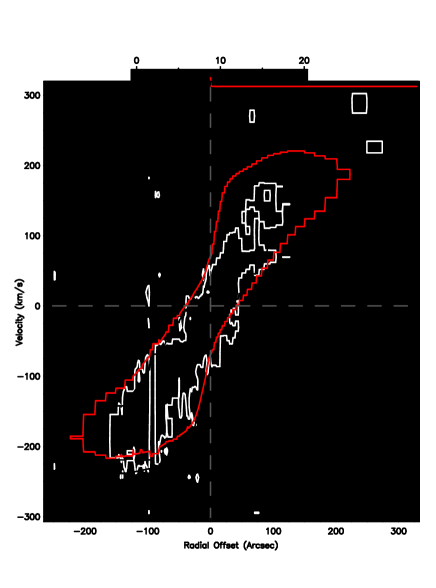
Figure 13: Color plot of the H$\alpha$ PV-diagram at 26-34 arcsec (1.2-1.6 kpc) offset from the major axis. Contours are at 3 $\sigma$. The white solid contour is the data, black contour is the best fit model (Model 3, Table2), red contour is the best fit model with an assumed vertical gradient of 16.5 km s^-1 kpc^-1 in the rotation curve (Model G3), Table 2.

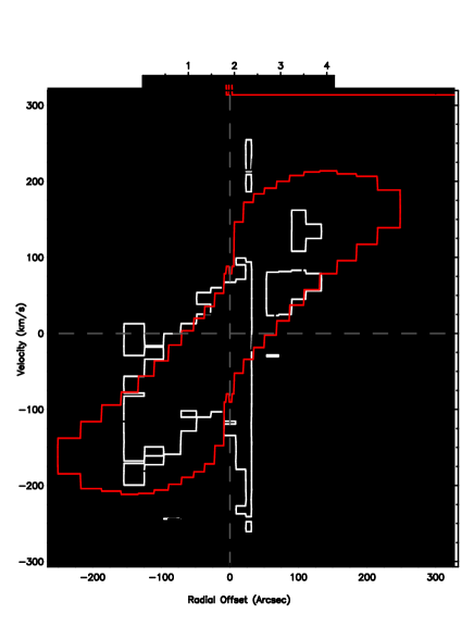
Figure 14: Same as Fig. 13 except now for the bin 48-67 arcsec (2.2-3.1 kpc) offset from the major axis.

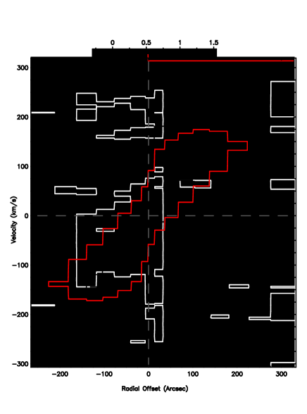
Figure 15: Same as Fig. 13 except now for the bin 68-107 arcsec (3.2-4.9 kpc) offset from the major axis.

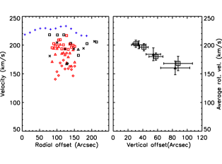
Figure 16: (Left) Results of employing envelope tracing to the data. Blue (pluses): HI on the major axis (Fraternali et al., 2005), red: points found by Heald et al. (2006), at vertical offsets $\sim$ 30 arcsec (squares), $\sim$ 50 arcsec (triangles) and $\sim$ 80 arcsec (diamonds). Black: our data at vertical offsets of 30 arcsec (squares), 40 arcsec (crosses), 58 arcsec (triangles) and 88 arcsec (diamonds). (Right) The average rotational velocity obtained with envelope tracing at a vertical offset of 30, 40, 58 and 88 arcsec (1.4, 1.9, 2.7 and 4.1 kpc) for our data (squares) and average points as obtained by Heald et al. (2006) at vertical offsets $\sim$ 30, 50, 80 arcsec (1.4, 2.4, 3.7 kpc)(triangles).

Figure 13 shows that the general slope of the diagram steepens compared to PV-diagram at the major axis. This is as we would expect since the gas is less obscured by the dust above the plane. Therefore, we can look farther into the galaxy and look at gas closer to the line of nodes. This steepening is also the reason why a thin annulus in the outer parts of the galaxy (See $\S$ 6.1) is very unlikely. In such a distribution this steepening would not be possible unless the gas of the annulus would move inward as it rises above the plane. Such an effect seems highly unlikely.
     If we compare the data to Model 3 we see that the steepening is not enough. Our model has much more gas at high velocities near the center of the galaxy. This lack of gas at the high velocities in the center might still be an effect of the dust but could also indicate that the rotational velocities of the gas above the plane not only lag compared to the disk but that the rotation curve rises less steep radially the higher we look above the plane.
     A close inspection of Figure 13 shows us that there are two more places where the data deviate from the model. The model underestimates the intensities at low velocities and overestimates them at high velocities. The lack of gas at high velocities at all radii confirms the lagging rotation curve found by Fraternali et al. (2005) and Heald et al. (2006). If we draw a straight line through the lower part of the 3$\sigma$ contour of the data and and then draw a straight line through the same contour of Model 3 we can measure the lagging of the halo. In this way we find a difference between Model 3 and the data $\sim 18.75\pm 6.3$ km s^-1 at a vertical offset of 30 arcsec (1.4 kpc).
     In the diagram that shows the gas at an offset of 60 arcsec (Fig. 14) we see that the slope of the emission becomes less steep compared to the slope at 30 arcsec. This is the continued effect of the rotation curve rising less steeply with radius the further we get from the plane. For this effect to be caused by dust the dust extinction would have to increase again which seems highly unlikely.
      From Figure 14 we find a difference between Model 3 and the data, by comparing the 3$\sigma$ contours, of $62.5\pm 6.3$ km s^-1. At this height we cannot be completely certain we are looking at the flat part of the rotation curve. Therefore, these effects could also be caused by radial redistribution of the gas. We consider it unlikely that such a redistribution completely causes the changes of the observed PV-diagram because intensity cuts parallel to the major axis only show a hint of such an effect and only at the East side of the galaxy, as shown by Heald et al. (2006) (their Fig. 7), while the West side is the brighter side of the halo.
      Figure 15 shows the gas at 90 arcsec offset from the major axis. The emission of the diffuse gas at this height is very low and we had too compare the 1$\sigma$ contours of the model and the data. Therefore conclusions drawn from this plot are considered to be no more than indicative. At this vertical offset the effects observed at a 60 arcsec offset continue. Comparing the highest velocity of the 1$\sigma$ contour at this height with Model 3 we observe a difference of $81.25\pm 12.5$ km s^-1.
     When we assume that the gradient starts on the major axis we find the slope of the gradient to be $\sim 18.8\pm 6.3$ km s^-1 when we fit the points at 30, 60 and 90 arcsec (1.4, 2.7 and 4.1 kpc).
      After determining the gradient of the lag we constructed a model (Model G3, see Table 2) in which the rotation curve is scaled down at higher $|z|$ by subtracting at every vertical step in the model $|z|\times 18.8$ km s^-1, with $|z|$ in kpc, from the rotation curve as obtained from the HI. The vertical step size in the model was 49 pc (1.05 arcsec). Model G3 is plotted in Figs. 13, 14 and 15 as the red contours. We see that gas is still missing at various places in the diagram but that the maximum and minimum velocities are approximately the same for the data as this model at the 3$\sigma$ contour. Thus confirming that there is a gradient of -18.8$\pm$6.3 km s^-1 kpc^-1 in the observations. The explanation for the missing gas remains the same as before since we did not change the shape of the rotation curve.

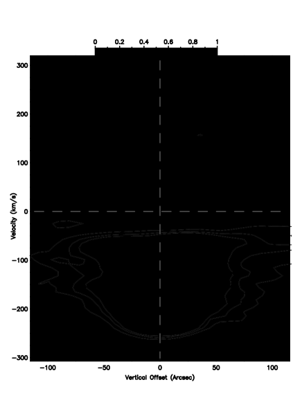
Figure 17: Normalized color plot of the H$\alpha$ PV-diagram at a radial offset of 150 arcsec parallel to the minor axis and overlaid with contours of HI at 3$\sigma$, 6$\sigma$ and 9$\sigma$.

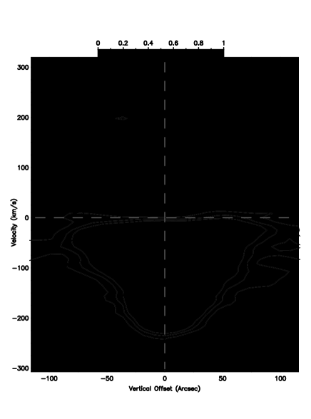
Figure 18: Same as 17 but now at a radial offset of 75 arcsec.

Figure 19: Same as 17 but now at the minor axis position.

Another way to look at the kinematics at higher $|z|$ is by constructing PV diagrams along the minor axis and parallel to the minor axis at some radial offset. To optimize the information in the diagrams we normalized them by dividing every line profile by it’s maximum. Figure 17 is an example of such a PV-diagram. This PV-diagram is constructed by looking through the cube at a radial offset of 150 arcsec and is a cut parallel to the minor axis. Overlaid on the color scale are the 3, 6, 9 $\sigma$ contours of the HI. Looking at this plot the first thing we see is that the HI is much more extended vertically than the H$\alpha$. This is partly due to beam smearing but not completely. If we look at the H$\alpha$ at low mean velocity ($\sim|140|$ km s^-1) we see that in the plane of the galaxy (e.g. 0 offset) the maximum of the emission lies at this low mean velocity. Moving away from the plane the maximum of the emission first rises to higher mean velocities and then drops again. The initial rise is caused by diminishing dust attenuation. As we move further from the plane the maximum of the emission drops to lower mean velocities again. This drop is caused by the lower rotational velocities at higher $|z|$. The H$\alpha$ is much less extended than the HI, in velocity as well as vertical size ($z_{\rm EM}$=0.5 kpc (Dettmar, 1990), the ionized gas scale height is twice this, $z_{\rm HI}$=2.3 kpc (T.Oosterloo, priv. communication)). Considering the sensitivity of both observations it could well be that our H$\alpha$ observations are just not sensitive enough to observe all the ionized gas in the galaxy. We also plot PV diagrams parallel to the minor axis at a offset of 75 arcsec and on the minor axis itself, Figures 18 and 19 respectively. In the figure at 75 arcsec offset from the minor axis we see the same behavior as at 150 arcsec offset, only here the rise and drop in mean velocities is much more extreme. We also see that in this diagram the mean velocity at the highest offset from the plane drops back towards systemic. This difference is caused by the rotation curve which rises less steep the further we look above the plane. Looking at the diagram which is a cut along the minor axis of the galaxy (Fig. 19) we see that here the maximum of the H$\alpha$ emission lies one channel below systemic velocity at almost all the offsets from the plane. This offset is about 18 km s^-1 which is larger than the error in the wavelength calibration (e.g., 6 km s^-1). We are confident this offset is not an error in our velocity scale. In principle we could check this by comparing the flat rotation speeds on the North side to those on the South side but we think such a check is unreliable due to the effects of dust on the South side.
     The flat shape in Figure 19 is as expected; the offset from systemic is unexpected. We realize that our central position of the galaxy is somewhat to the south from the central position generally used in kinematical studies, but notice that shifting the central position to the north would further remove us from the kinematical center of the H$\alpha$. Also our kinematical center and the center used in this paper would lie in the same resolution element of the HI observations. We note that at a vertical offset of $\sim$ 60 arcsec the maximum seems to be displaced more from the systemic velocity. This is a real effect and is not caused by our way of binning the data. Whether this deviation is important for understanding the general dynamics of the halo remains unclear.

7 Summary

We present Fabry-Pérot H$\alpha$ measurements of the edge-on galaxy NGC 891. This is the first time kinematical data for the H$\alpha$ are presented for the whole of NGC 891.
     In our observations we can clearly see H$\alpha$ emission above and below the plane of NGC 891. This vertical extent is already visible in the separate channel maps and becomes even more obvious in a velocity integrated map.
      This integrated velocity map shows a clear contrast between the distribution of the H$\alpha$ on the North-East and the South-West side of the galaxy. This dichotomy is not restricted to the plane of the galaxy but is also clearly visible above the plane. Since dust absorption is negligible above the plane it is likely that this dichotomy is a real physical effect. Assuming that the halo gas is brought up from the plane by a SFR related mechanism, this implies that the SFR on the South-West side of the galaxy is much lower than on the North-East side of the galaxy.
     For the interpretation of the kinematics of the extra-planar gas we constructed several 3-D models of an exponential disk rotating with a rotation curve derived from the HI data (Fraternali et al., 2005). Included in the models is a uniform dust layer of given optical depth distributed exponentially in radius and height and a truncation radius.
     We started with models that have the same scale length for the dust disk as the H$\alpha$ disk ($h_{\rm g}=h_{\rm d}=5$ kpc). We find that such models generate too much intensity at large radii and high velocities when we compare them to the data. To overcome this problem we modeled the galaxy with a dust scale length of 8.1 kpc, as derived by Xilouris et al. (1998) from observations in the V-band. The longer scale length of the dust reduces the intensity of the gas at large radii and high velocities. This also provides us with a upper limit scale length of the ionized gas of 6.5 kpc (Model 1.1). Longer scale lengths would reintroduce the too high intensities found in the first models. A lower limit is found for a model with a scale length of 2.5 kpc (Model 2.2). Models with even shorter scale lengths do not produce enough intensity at large radii. Better constrains could be obtained if the truncation radius of the dust disk would be known.
      When we fit models in this range to the PV-diagram of the major axis we find that the best fit is a model with a central attenuation of $\tau_{\rm H\alpha}=6$, a cut off radius $R_{\rm max}=14$ kpc and a scale length and height of 5.0 kpc and 0.8 kpc respectively (Model 3). By comparing PV-diagrams above the plane to the models kinematical information about the galaxy is extracted from the data. We confirm the lagging of the halo, as found by Fraternali et al. (2005) and Heald et al. (2006), and determine that this lagging occurs with gradient of $\sim 18.8\pm 6.3$ km s^-1 kpc^-1.
      In the PV-diagrams we also see that compared to the models the distribution of the H$\alpha$ is displaced to larger radii or lower rotational velocities. This effect increases as we look higher above the plane. This means that the higher we look above the plane, the less steep the rotation curve rises. We can confirm this by comparing three cuts through the cube along and parallel to the minor axis. After normalizing these PV-diagrams we can clearly see that the H$\alpha$ at a distance of 75 arcsec from the center has a larger gradient than the H$\alpha$ at 150 arcsec from the center.