The ZEPLIN II dark matter detector: data acquisition system and data reduction

Abstract

ZEPLIN II is a two-phase (liquid/gas) xenon dark matter detector searching for WIMP-nucleon interactions. In this paper we describe the data acquisition system used to record the data from ZEPLIN II and the reduction procedures which parameterise the data for subsequent analysis.

, , , , , , , , , , , , , , , , ,, , , , , , , , , , , , , , , , , , , , , , , , , , , , , , , , , , , , , , , ,

1 Introduction

The ZEPLIN II dark matter detector has been operational at the Boulby Mine underground laboratory since 2005. Its principle aim is to detect and measure the faint nuclear recoil signal from galactic Weakly Interacting Massive Particles (WIMPs). ZEPLIN II is a two-phase (liquid/gas) xenon detector which has an increased sensitivity over previous UK Dark Matter Collaboration experiments NaIAD [1] and ZEPLIN I [2]. By measuring both the primary and secondary scintillation signals produced by particles interacting in the target volume [3, 4, 5] this technique has the potential to improve discrimination between nuclear recoils expected from WIMP interactions (also produced in neutron collisions with nuclei) and electron recoils (caused by $\gamma$-rays and electron interactions, e.g. $\beta$-particles). The differential energy spectrum of these nuclear recoil events is expected to be featureless and smoothly decreasing with detected recoil energies which are less than 100 keV for WIMP masses in the range 10-1000 GeV c² [6]. Dark matter experiments need to be capable of detecting recoil energies of a few keV in order to place the most stringent limits on the rate of WIMP interactions. In scintillator experiments this requires sensitivities to single photoelectrons. Due to the extended waveform digitisation and fine resolution, a large volume of data is collected ($\sim$8 TBytes/yr, excluding calibration data). The data requires efficient processing and must be stored for subsequent analysis. Reduction procedures capable of parameterising the data have been developed to process the waveforms and output a set of parameters representative of the original waveform.

In this paper we present a brief description of the detector followed by a more detailed discussion of the data acquisition system and data reduction procedures. In our companion paper [7] we present initial results from the first underground run of ZEPLIN II.

2 The Detector

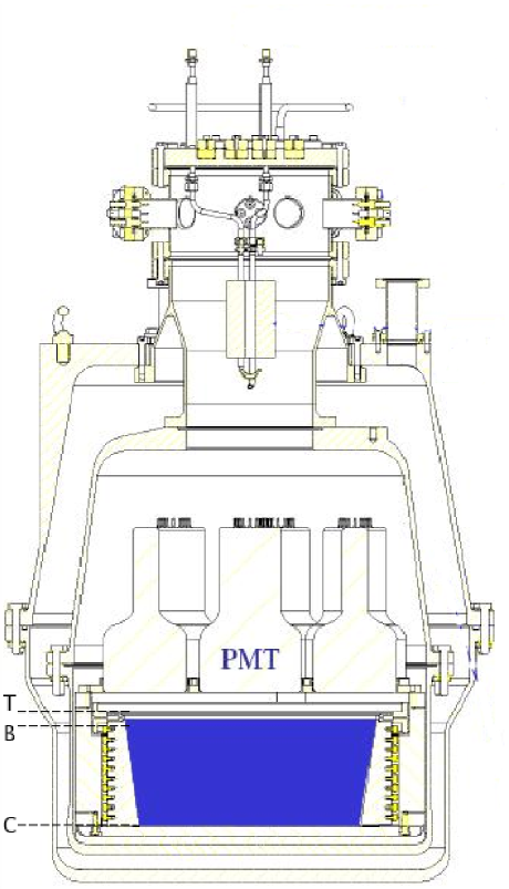
Figure 1: Schematic of ZEPLIN II showing the relative positions of the electric field grids and the liquid/gas interface where T is top grid, B is bottom grid and C is the cathode.

ZEPLIN II consists of 31 kg of liquid xenon contained in a 50 cm diameter copper vessel (Figure 1). The target volume is viewed from above by 7 ETL D742QKFLB 130 mm photomultiplier tubes (PMTs) in a close-packed hexagonal pattern. Two steel grids and a mesh act as electrodes which define the electric field in the detector. Two of the grids are positioned above and below the liquid surface; these are the top and bottom grids which define the electroluminescence and charge extraction fields. The wire mesh is located at the bottom of the target defining the drift field in the active volume of the target. PTFE lining the inside of the copper vessel acts both as a support structure for the high voltage grids and a reflector. The target is maintained at liquid xenon temperature by an IGC PFC330 Polycold system [8]. Circulation of the xenon through SAES getters (model PS11-MC500) [9] ensures impurities do not reduce the performance of the target. The copper vessel is surrounded by a stainless steel jacket which provides an insulating vacuum. The detector sits in a liquid scintillator veto system viewed from above by 10 ETL 9354KA 200 mm PMTs. The upper half of detector/veto system is surrounded by hydrocarbon slabs (separated by Gd-loaded resin sheets) shielding the target from external background neutrons (the liquid scintillator veto acts as its own neutron shield). The entire apparatus is housed in a lead “castle” which shields against external background $\gamma$-rays.

In normal (two-phase) operating mode ZEPLIN II is designed to detect the vacuum ultra-violet scintillation and ionisation charge signal of an interacting particle. The scintillation light comes from the initial particle interaction (prompt de-excitation of Xe${}_{2}^{*}$ dimer to dissociative ground state). Under an applied electric field, a fraction of the ionisation electrons are drifted to the liquid surface where they are removed by the extraction field into the gas phase producing a secondary scintillation pulse through electroluminescence. We adopt the convention of naming the primary and secondary signals S1 and S2 respectively.

The region between the bottom grid and the cathode defines the active volume of the detector and contains a drift field of $\sim$1 kV/cm. The electron drift velocity in this region is about 2.0 mm/$\mu$s. Field shaping rings embedded in the PTFE support structure keep the drift field lines parallel. The top grid defines both the extraction and electroluminescence fields in the region between the top and bottom grids. The time delay between the S1 and S2 signals permits the depth of the particle interaction to be reconstructed.

3 Data Acquisition System

Figure 2 shows the signal path from PMT to the data acquisition system (DAQ). PMT gains are equalised to give about 4.5 mV per photoelectron (pe) output. The 7 PMT signals from the target are first passively split by a 50 $\Omega$ splitter: one line is fed to a $\times$10 amplifier, the other to the signal input of the DAQ (channels ACQ1 to ACQ7 in Figure 2). From the amplifier the signals are fed to discriminator D1 which outputs 50 mV/channel for input signals above 17 mV (approximately 2/5 of the spe signal). The logic sum of the signals is then fed to discriminator D2 which outputs a NIM pulse to dual timer T2 when 5 out of 7 PMTs detect a signal above the 17 mV threshold level. At the same time, T2 sends a 100 $\mu$s square-wave pulse to the veto input of D1 to prevent further triggers until the whole waveform is read by the DAQ. The amplified signal from the central PMT (PMT 1) is also attenuated before going into discriminator D3. Due to the relative placing of the PMTs and the PTFE support/reflector structure, the central PMT sees a larger signal (on average) than the outer PMTs. Large amplitude signals can cause optical feedback in the target giving rise to many noise pulses of long duration. Signals exceeding a pre-set threshold of 200 mV (see below for explanation) are vetoed by the dual timer T2 which sends a 1 ms inhibit signal to D1 to prevent optical feedback signals from triggering the system. This also has the effect of reducing the trigger rate by 60%, reducing data processing and data storage requirements. The 10 PMT signals from the veto feed 10 channels of a discriminator/buffer NIM module. The sum of the discriminator outputs is passed into a second discriminator whose threshold is set to output a logic pulse if at least 3 of the veto PMTs fire in coincidence. This pulse is delayed by 100 ns in a delay line and the output is added to the analog sum of the veto PMT outputs.

The waveform hardware consists of DC265 M2M ACQIRIS digitizers embedded in CC103 ACQIRIS [10] crates. These are based on CompactPCI technology interfaced through the PCI bus. The digital conversion of signals has an 8 bit resolution, a conversion rate of up to 500 MSamples/s, a bandwidth of 150 MHz and a memory of 2 MPoints/channel. Each 200 $\mu$s waveform is sampled at 2 ns intervals. LINUX-based software reads out the digitised waveforms which are then written to disc. Monitoring of all target parameters such as temperature and pressure is done with a 64 channel Datascan [11] module via the serial port on the DAQ computer.

Signals exceeding an amplitude of 200 mV are vetoed by the DAQ electronics. In addition, an upper cut of 180 mV is implemented in software. Signals above this threshold are above the energy range of interest for dark matter searches but the effect, in terms of efficiency, must be estimated. Figure 3 shows the efficiency as a function of energy calculated from data taken with and without the software threshold - but keeping the additional 200 mV saturation cut on the central PMT in both cases. The efficiency is 100% up to 30 keV.

In order to investigate the fraction of events lost due to DAQ dead time dedicated pulser measurements were performed. The pulser was set to output a pulse of amplitude 0.81 V with 0.2 ms duration. For a waveform of 100,000 samples at 2 ns per sample the maximum recordable rate was 22 Hz, corresponding to a dead-time of $\sim$50 ms. In a non-paralyzable model, where events occuring during dead periods do not extend the dead-time, the measured event rate $n$ is given by $n=m/(1-m\tau)$ [12], where $m$ is the observed event rate and $\tau$ is the dead-time. The typical observed background rate in the target is 2 Hz which corresopnds to a loss of $\sim$10% of events (since $m/n=1/(1-n\tau)$). For data taken with an AmBe neutron source located approximately 1 m above the target the true event rate was 34.4 Hz which corresponds to a loss of 67%. For a ⁶⁰Co source located in the same position the loss was 78% with a true event rate of 70 Hz.

4 Data Reduction

A raw data file with 2000 events is approximately 250 MB compressed (each waveform has 100,000 points and there are 7 PMT channels plus 1 veto channel for each event). Approximately 25 GB of data (excluding calibration runs) is recorded each day. The data are then written to magnetic digital tape on an ADIC Scalar 100 tape robot system [13]. Each tape can store 100 GB of data. The data are subsequently transferred to an Apple XGrid capable of reducing $\sim$0.6 TB of data per day.

Raw data are reduced with a LINUX-based application which reads in the binary data files and outputs a set of numeric parameters representing each pulse found on each waveform. The software consists of an event viewer, allowing the examination of each trace in each PMT and reduction algorithms which process the waveforms from each channel. All peaks in each waveform must be identified and parameterised according to height, width, area and time-constant. Pulse parameters are then written to reduced data files in HBOOK ntuple format [14] for subsequent analysis. The user must specify a number of input variables for the peak-finding algorithms, these are discussed in turn.

4.1 Input Parameters

Different length signal cables from the PMTs to the DAQ and differing PMT characteristics can induce delays in the pulse arrival times in each channel. In addition, differences in transit times in the PMTs can induce delays up to $\sim$40 ns. Pulses detected coincidently in several channels can appear spread out in the summed waveform if these delays are not corrected. This can lead to peaks in the summed waveform being incorrectly parameterised as separate pulses. Figure 4 shows the distribution of pulse mean arrival times in each PMT relative to the central PMT (PMT 1) for uncorrected data. Channels are shifted in software by their delay with respect to PMT 1 and the summed waveform calculated.

To facilitate peak-finding a smoothing function is applied to the summed waveform. This ensures that small amplitude fluctuations do not get mis-identified as valid signal pulses. The amplitude $h_{t}$ at each sample is smoothed as

$$S_{t}=\frac{\sum_{t=-t_{sm}/2}^{t_{sm}/2}{h_{t}}}{N_{-t_{sm}/2}^{t_{sm}/2}}$$ (1)

where $t_{sm}$ is the smoothing timescale and is an input parameter to the reduction. Figure 5 shows a single photoelectron spectrum from the central PMT parameterised with different values of $t_{sm}$ from 5 ns up to 50 ns. The larger value of $t_{sm}=50$ ns can be seen to ’wash-out’ lower energy pulses resulting in a shift in the peak of the spectrum to higher energies. A value of $t_{sm}=12$ ns was chosen as it correctly reproduces the mean value of the spe calibrations.

All pulses above a user-defined software threshold are tagged, up to a maximum of 10. The software threshold depends on the full-scale of the DAQ and is set to 2 mV (almost 1/2 pe) for data aquired with a full scale of 200 mV. This range was chosen as a compromise between energy resolution for S1 signals and the dynamic range for S2 pulses. The smoothed amplitude $h_{s}$ is used only to locate peaks on the summed waveform, all other parameterisation uses the unsmoothed original data.

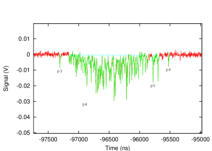
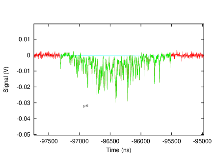
Figure 6: Ionisation pulse parameterised with 50 ns clustering (top) showing that four different pulses (p3 to p6) have been identified. With 400 ns clustering (bottom) these have been correctly grouped into a single pulse p6.

We define a clustering timescale which allows closely spaced peaks on the waveform to be grouped together to form a single pulse. A low energy S2 signal can appear as separate peaks spread out over several $\mu$s (the total width of S2 is determined by the distance between the top grid and the liquid surface). Figure 6 shows the effect of different clustering values on the same pulse. A clustering of 50 ns causes peaks p3, p5 and p6 to be identified as separate pulses from p4. Increasing the clustering timescale to 400 ns correctly groups all peaks as a single pulse.

4.2 Output Parameters

The baseline for each waveform is calculated on an event-by-event and channel-by-channel basis. An initial baseline is calculated from the mean of the first 500 data points. However, this is not sufficient because the baseline tends to wander bay a few mV during the event. A box-car smoothing algorithm with a width of 5000 ns is used to calculate a wandering baseline to compensate for this effect. As the wandering baseline is calculated, any data point deviating by more than 5$\times$ the RMS noise from the current value of the baseline is excluded from the baseline calculation. This prevents the wandering baseline from following the slow S2 signals from the gas phase of the data.

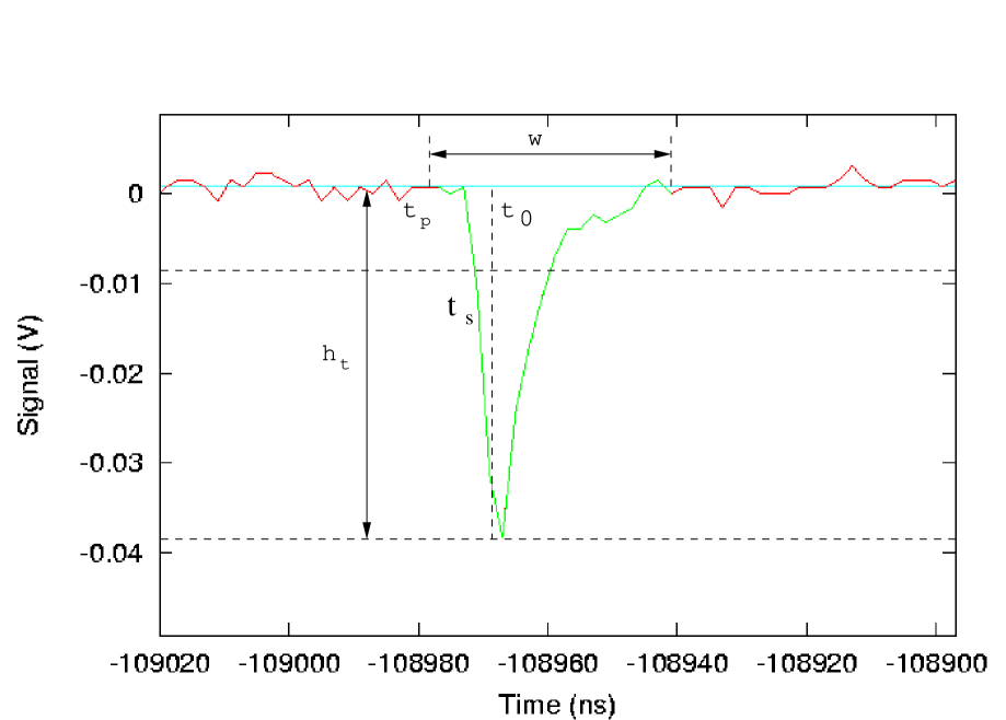
Figure 7: Basic pulse parameters. $h_{t}$ is the signal amplitude above the baseline, $t_{p}$ is the start time of the pulse and $t_{0}$ is the time at which 10% of the total charge has arrived. $w$ is the pulse width defined by the start and end time of the peak.

An initial scan is made of the waveform on the sum channel for pulses with amplitudes above the software threshold. The start time of each pulse $t_{s}(i)$ (see Figure 7) where $i$ is the index of the pulse (up to the maximum of 10) is then used to find the proper start time of the pulses $t_{p}(i)$ on the baseline. The difference between the end and start time defines the pulse widths $w(i)$. Once all pulses on the summed waveform are identified, each individual channel is scanned in the time windows $w(i)$. Each $t_{p}(i)$ is used to define a time $t_{0}(i)$, at which 10% of the total charge of the pulse is detected. This is then used to calculate the charge mean arrival time $\tau$ as in Equation 2.

$$\tau=\frac{\sum_{t=t_{0}}^{t_{p}+w}{h_{t}.(t-t_{0})}}{\sum_{t=t_{0}}^{t_{p}+w}{h_{t}}}$$ (2)

where $h_{t}$ is the largest amplitude within the time window. The FWHM of the pulse is calculated starting from the time at which $h_{t}$ is observed and tracing outwards in both directions to the times at which the pulse height falls to $h_{t}/2$. Another measure of the full width half maximum (LFWHM) is calculated by tracing the pulse height to its half maximum value by starting at both the beginning and end of each pulse.

The RMS noise of the waveform is the mean deviation of the data from the baseline in the pre-trigger region.

$$N_{RMS}=\sqrt{\frac{\sum{h_{t}}^{2}}{N}}$$ (3)

Pulse area $A$ (in units of nV.s) is defined as the integrated area of the pulse in the time window and is intended as the best measure of the total charge associated with the pulse.

$$A=\sum_{t=t_{p}}^{t_{p}+w}{A_{t}}$$ (4)

The summed veto signal is parameterised according to its height, arrival time and total integrated charge following the same procedure for signal pulses from the target. Table 1 lists all pulse parameters calculated.

5 Data Analysis

Reduced data files consist of parameters for each pulse found on each of the 7 PMT channels defined by those pulses found on the sum channel. All parametersied waveforms must be analysed to extract the required S1 and S2 signals. The secondary ionisation signal will be delayed from the primary scintillation signal by an amount which depends upon the depth of the interaction in the target. The drift velocity of ionistation electrons (which is determined by the drift field) is typically 2.0 mm/$\mu$s. The longest drift time is the time taken for ionisation electrons from the cathode to reach the bottom grid and is about 75 $\mu$s. Since the DAQ can trigger on either the S1 or S2 signal, waveforms are recorded 100 $\mu$s on each side of the trigger position. The waveform time window was chosen to be [-200,0] $\mu$s with the trigger at -100 $\mu$s. Events which trigger on the primary will have a secondary signal in the range [-100,0] $\mu$s and those events which trigger on the secondary will have a primary scintillation signal in the range [-200,-100] $\mu$s. In either case, secondary ionisation signals only occur in the range [-100,0] $\mu$s. The first step in the analysis involves scanning this region for pulses on the sum channel which are greater than 1 V.ns in energy (see below). All pulses greater than 1 V.ns in this range are tagged as possible S2 signals. Next, the [-200,-100] $\mu$s region of the wavefom is scanned for the primary sciltillation pulse. Coincident pulses with an amplitude greater that 1.7 mV in any 3 out of 7 channels are tagged as possible S1 candidates. An additional cut of $\tau>150$ ns for S2 and $2\,$ns $<\tau<50$ ns for S1 is applied (the efficiencies for these and other selection criteria are discussed in [7]). We reject those events with more than 1 S2 signal as WIMPs do not multiple scatter. We also reject events with more than 1 primary scintillation pulse. All events with only one S1 and only one S2 are accepted.

The 1 V.ns selection criteria ensures that small single electron signals do not get mis-identified as S2. Figure 8 shows a typical cluster of single electron pulses spread over 600 ns with a total energy of 0.5 V.ns. Each peak appears in different channels at different times (not shown) but the clustering parameter groups them together in a single pulse. Low energy nuclear recoils are expected to produce more than one ionisation electron so the probability of rejecting genuine S2 signals is low. To investigate this further, we plot the distribution of S2 for S1 in a restricted energy range in Figure 9. The distribution peaks at $\sim$10 V.ns and is roughly Gaussian in shape with a noise contribution impinging on the distribution from the left. Fitting an exponential plus Gaussian to the S2 spectrum allows us to calculate the efficiency of the 1 V.ns cut by integrating the area of the Gaussian above 1 V.ns and dividing by the total area. Requiring a minimum of 1 V.ns for S2 results in loss of approximtely 8% of events (92% efficiency) between 5-10 keV. However, the fitted Gausian extends to below zero, which is unphysical, and so this loss is overestimated. For higher energies the efficiency is close to 100%.

To convert the observed pulse energy (in mV) to electron equivalent energy (in keV) calibrations were performed with a ⁵⁷Co (two spectral lines at 122 keV and 136 keV) source located beneath the target volume and delivered by a dedicated source delvivery mechanism. 10,000 events were recorded with waveforms 200$\mu$s in duration and with a drift field of 1 kV/cm. S1 and S2 signals were extracted from the parameterised data as described. Figure 10 shows the calibration spectrum with a fit to the peak at 2.54 V.ns. This corresponds to $\sim$67 pe (1 pe $\approx$ 0.038 V.ns) which gives a light-yield of $\sim$0.55 pe/keV for this data. This corresponds to $\sim$ 1.1 pe/keV at 0-field assuming a 50% scintillation-yield loss with a drift field of 1 kV/cm.

6 Summary

We have described the data acquisition system for the ZEPLIN II dark matter experiment which uses ACQIRIS digitizers to record the event waveforms from the detector. Approximately 8 TB of dark matter data per year are recorded. Data reduction procedures have been developed to parameterise the data; up to 0.6 TB of data per day can be reduced.

7 Acknowledgements

This work has been funded by the UK Particle Physics And Astronomy Re- search Council (PPARC), the US Department of Energy (grant number DE- FG03-91ER40662) and the US National Science Foundation (grant number PHY-0139065). We acknowledge support from the Central Laboratories for the Research Councils (CCLRC), the Engineering and Physical Sciences Research Council (EPSRC), the ILIAS integrating activity (Contract R113-CT-2004- 506222), the INTAS programme (grant number 04-78-6744) and the Research Corporation (grant number RA0350). We also acknowledge support from Fun- dao para a Cincia e Tecnologia (pro ject POCI/FP/FNU/63446/2005), the Marie Curie International Reintegration Grant (grant number FP6-006651) and a PPARC PIPPS award (grant PP/D000742/1). We would like to grate- fully acknowledge the strong support of Cleveland Potash Ltd., the owners of the Boulby mine, and J. Mulholland and L. Yeoman, the underground facil- ity staff.

Table 1: Waveform parameters calculated by reduction procedure.

Parameter	Explanation
$B$	Baseline level for each channel
$N_{RMS}$	RMS noise level for each channel
$t_{p}$	Start time of all pulses on each waveform
$t_{0}$	Time of arrival of 10% of the pulse charge
$w$	Width of each pulse in each channel
$A$	Area of each pulse in each channel
$h$	Height of each pulse in each channel
$FWHM$	Pulse FWHM measured from maximum pulse height
$LFWHM$	Pulse FWHM measured from pulse start and pulse end time
$\tau$	Charge mean arrival time
$t_{v}$	Start time of veto pulse
$h_{v}$	height of veto pulse
$A_{v}$	Integrated area of veto pulse

Figure 2: Signal path from target and veto PMTs to DAQ via trigger electronics.

Figure 3: Software saturation cut efficiency as a function of energy. Efficiency is 100% up to 30 keV.

Figure 4: Mean signal delay $\Delta_{1i}$ between PMT 1 and PMT i. The $\Delta_{1i}$ are 3.927 ns, 7.941 ns, 8.737 ns, 10.07 ns, 6.294 ns and 6.916 ns for $i=2\ldots 7$ respectively.

Figure 5: Single photoelectron spectra for PMT 1 with different values of $t_{smooth}$: 5 ns (dashed line), 12 ns (solid line), 20 ns (dotted line) and 50 ns (dash-dot line). The spectrum peaks at $\sim$0.035 pe/keV

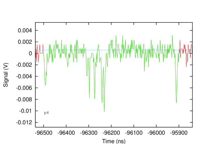
Figure 8: Typical noise event due to single electrons extracted from the liquid giving rise to an electroluminescence signal in the gas.

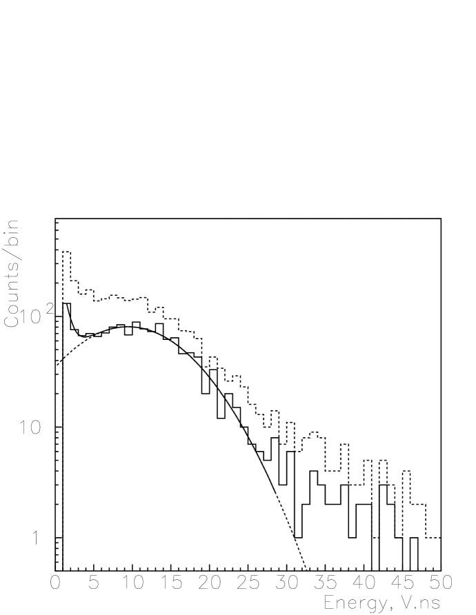
Figure 9: AmBe S2 distribution for S1 between 5 keV and 10 keV (dashed histogram). The solid histogram is the distribution excluding events near the top and bottom grids. Superimposed is the Gaussian fit (plus exponential noise) to the data.

Figure 10: Energy spectrum from ⁵⁷Co calibration run with a drift field of $\sim$1 kV/cm in the target. A fit of two Gaussians to the main peak returns the position for the 122 keV line at 2.54 V.ns.

References

- [1] G.J.Alner et al., Phys. Lett. B 616 (2005) 17-24.
- [2] G.J.Alner et al., Astropart. Phys. 23 (2005) 444-462.
- [3] G.J. Davies et al., Phys. Lett. B 320 (1994) 395.
- [4] H. Wang, PhD Thesis, UCLA, 1999.
- [5] D.B. Cline et al., Astropart. Phys. 12 (2000) 373.
- [6] J.D.Lewin and P.F.Smith, Astropart. Phys. 6 (1996) 87-112.
- [7] G.J.Alner et al. (2007), Submitted to Astroparticle Physics
- [8] www.polycold.com
- [9] www.saesgetters.com
- [10] www.acqiris.com
- [11] www.msl-datascan.com
- [12] G. F. Knoll, Radiation Detection and Measurement, third edition. Wiley
- [13] www.adic.com
- [14] wwwasdoc.web.cern.ch/wwwasdoc/ hbook_html3/hboomain.html