A longer XMM-Newton look at I Zwicky 1: Distinct modes of X-ray spectral variability

Abstract

The short-term spectral variability of the narrow-line Seyfert 1 galaxy I Zwicky 1 (I Zw 1) as observed in an $85{\rm\thinspace ks}$ XMM-Newton observation is discussed in detail. I Zw 1 shows distinct modes of variability prior to and after a flux dip in the broad-band light curve. Before the dip the variability can be described as arising from changes in shape and normalisation of the spectral components. Only changes in normalisation are manifested after the dip. The change in the mode of behaviour occurs on dynamically short timescales in I Zw 1. The data suggest that the accretion-disc corona in I Zw 1 could have two components that are co-existing. The first, a uniform, physically diffuse plasma responsible for the “typical” long-term (e.g. years) behaviour; and a second compact, centrally located component causing the rapid flux and spectral changes. This compact component could be the base of a short or aborted jet as sometimes proposed for radio-quiet active galaxies. Modelling of the average and time-resolved rms spectra demonstrate that a blurred Compton-reflection model can describe the spectral variability if we allow for pivoting of the continuum component prior to the dip.

1 Introduction

There is strong evidence that the accretion processes in Galactic black holes (GBHs) and active galactic nuclei (AGNs) are similar within some scaling relation (e.g. Merloni et al. 2003; McHardy et al. 2006). It would then follow that the various states and types of spectral variability seen in GBHs (see Remillard & McClintock 2006 for a recent review) should also be present in AGNs. Here we study a spectral variability mode change in the AGN I Zwicky 1 (I Zw 1; $z=0.0611$).

In the standard model a transition from one state to another in GBHs is normally attributed to a change in the geometry of the accretion flow and thus should occur on viscous timescales (e.g. Esin et al. 1998). In the high-soft state, a standard accretion disc (Shakura & Sunyaev 1973) extends down to the last stable orbit and dominates the X-ray emission. In the low-hard state the standard disc is truncated at a few 100 gravitational radii (${\thinspace r_{\rm g}}=GM/c^{2}$) and hard, non-thermal emission from a low-efficiency accretion flow dominates. Identifying similar behaviour in $\sim 10^{7}\hbox{$\rm\thinspace M_{\odot}$}$ AGNs is difficult as the characteristic timescales are $10^{6}$ times longer than for a $10\hbox{$\rm\thinspace M_{\odot}$}$ GBH.

The low-hard state is also associated with radio emission from a jet, which dissipates as the GBH enters the high-soft state (Gallo et al. 2003). This has led to the concept that much of the X-ray emission is from the base of a jet (e.g. Markoff, Falcke & Fender 2001; Ghisellini, Haardt & Matt 2004). Moreover, Belloni et al. (1997) demonstrate that “blobs” of radio emission observed from the Galactic black hole GRS 1915+105 could be the inner accretion disc that is being evacuated from the system, giving rise to a truncated disc. On the other hand, Vadawale et al. (2003) show that this situation can also be realised if instead it is coronal material (i.e. hot plasma) that is ejected while the inner disc remains intact. In fact, Miller et al. (2006) show evidence of a broad iron line in the spectrum of GX 339–4 during a low-hard state indicating that an optically thick disc is present near the innermost stable circular orbit, in apparent disagreement with the standard model for state transitions. Therefore, some state changes may be associated with changes in the inner magnetic structure of the disc, which could occur faster than viscous timescales, rather than from modification of the accretion flow.

GBHs also exhibit much more rapid types of spectral and flux variations (e.g. McClintock & Remillard 2003). For example, in Greiner et al. (1996) GRS 1915+105 is shown to undergo fast oscillations of various amplitudes on timescales down to a few seconds. Catching a supermassive black hole exhibiting an analogous event over the course of an X-ray mission is likely, but even these events would occur on timescales longer than a typical XMM-Newton AGN observation.

The narrow-line Seyfert 1 galaxy (NLS1) I Zw 1 was observed with XMM-Newton (Jansen et al. 2001) at two epochs separated by approximately three years (Gallo et al. 2004a, 2007; hereafter G04 and G07, respectively). In G07 the mean spectral and timing properties of the 2005 observation were presented and changes in the spectral shape and intrinsic absorption (neutral and ionised) since the 2002 observation were reported (see Costantini et al. (2007) for a detailed presentation of the ionised absorber). Here we focus on the rapid spectral variability during the 2005 observation. Details of the observation and data processing are found in G07.

The black-hole mass ($M$) in I Zw 1 is log($M$/$\rm\thinspace M_{\odot}$)$=7.441^{+0.093}_{-0.119}$ (Vestergaard & Peterson 2006) and has a corresponding orbital period of $<3000s$ at $\sim 2{\thinspace r_{\rm g}}$ (${\thinspace r_{\rm g}}=GM/c^{2}$). The short-term variability exhibited by I Zw 1 could be portraying an observable state transition in an AGN. The change in the mode of behaviour in I Zw 1 is occurring on dynamically short timescales. Such variations would correspond to a few ms in GBHs and likely be unobservable as they would be too short. When normalised per unit crossing time, the count rates in AGNs are orders of magnitude larger than in GBHs.

2 The sharp flux dip in the 2005 X-ray light curve

During the 2002 observation of I Zw 1 the most notable feature in the light curve was a modest X-ray flare that was concentrated at high energies ($E\mathrel{\hbox{\hbox to0.0pt{\hbox{\lower 4.0pt\hbox{$\sim$}}\hss}\hbox{$>$}}}3{\rm\thinspace keV}$) (G04). In the 2005 light curve, I Zw 1 displays another distinct feature; this time a sharp flux dip occurs about $25{\rm\thinspace ks}$ into the observation (Fig. 1).

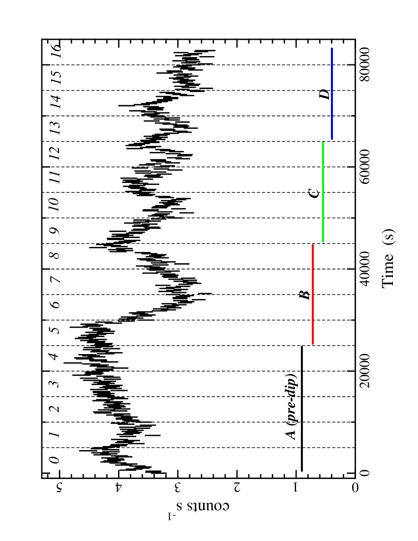
Figure 1: The 2005 $0.2-12{\rm\thinspace keV}$ EPIC pn light curve in $200{\rm\thinspace s}$ bins. The start time corresponds to the beginning of the pn exposure. The vertical dashed lines identify $5{\rm\thinspace ks}$ blocks of the observation and are numbered from $0-16$. Note that block 16 is not a full $5{\rm\thinspace ks}$ in length. The entire light curve is also separated into 4 segments, each consisting of $\sim 20-25{\rm\thinspace ks}$ of data, and labeled Seg A–D. Seg A comprises data prior to the sharp dip that starts at about $25{\rm\thinspace ks}$.

Though it is the most distinct characteristic in the light curve, the dip in count rates is a relatively modest event compared to the X-ray variability seen in some NLS1s (e.g. Boller et al. 1997; Brandt et al. 1999). However, of more interest is the clear change in behaviour that is associated with the dip. G07 already presented the onset of a time-lag between X-ray energy bands that coincided with the dip. Here, the focus will be on the different spectral variability that is exhibited during the pre- and post-dip phases. As will be demonstrated the flux dip represents a transition in the spectral behaviour of the AGN.

In order to examine the time-resolved behaviour of I Zw 1, the data were divided as shown in Fig. 1. Firstly, the data were separated into 17 blocks marked $0-16$ corresponding to $5{\rm\thinspace ks}$ intervals. As the live-time of the pn CCD in small-window mode is $71$ per cent, the net exposure in each $5{\rm\thinspace ks}$-interval is $\sim 3.6{\rm\thinspace ks}$. In block 16 the CCD was not active for the entire $5{\rm\thinspace ks}$ resulting in limited data and poorer signal than in the other blocks. Consequently, this block is omitted in the analysis if the shortage of data limits the constraints on model parameters. Secondly, the data were separated into 4 segments (labeled A–D), composed of 4 or 5 sequential blocks each, and identifying regions of particular interest. For example, Segment A constitutes blocks $0-4$, which includes all the data prior to the flux dip at $25{\rm\thinspace ks}$. Segment B includes blocks $5-8$, which consist of data during the dip. Segments C and D constitute post-dip data.

3 Pre- and post-dip: Distinct modes of variability

3.1 Hardness-ratio analysis

There are several lines of evidence demonstrating distinct spectral behaviour prior to and after the flux dip at $\sim 25{\rm\thinspace ks}$. Hardness-ratio ($HR=(H-S)/(H+S)$, where $H$ and $S$ are the count rates in the hard and soft bands, respectively) variability curves, such as that shown in Fig. 2 (left panel, $H=2.5-12{\rm\thinspace keV}$ and $S=0.5-1{\rm\thinspace keV}$), indicate that prior to the flux dip spectral variability (primarily spectral hardening) was taking place. After the dip, the $HR$ curve is consistent with a constant indicating no significant time-dependent spectral variability.

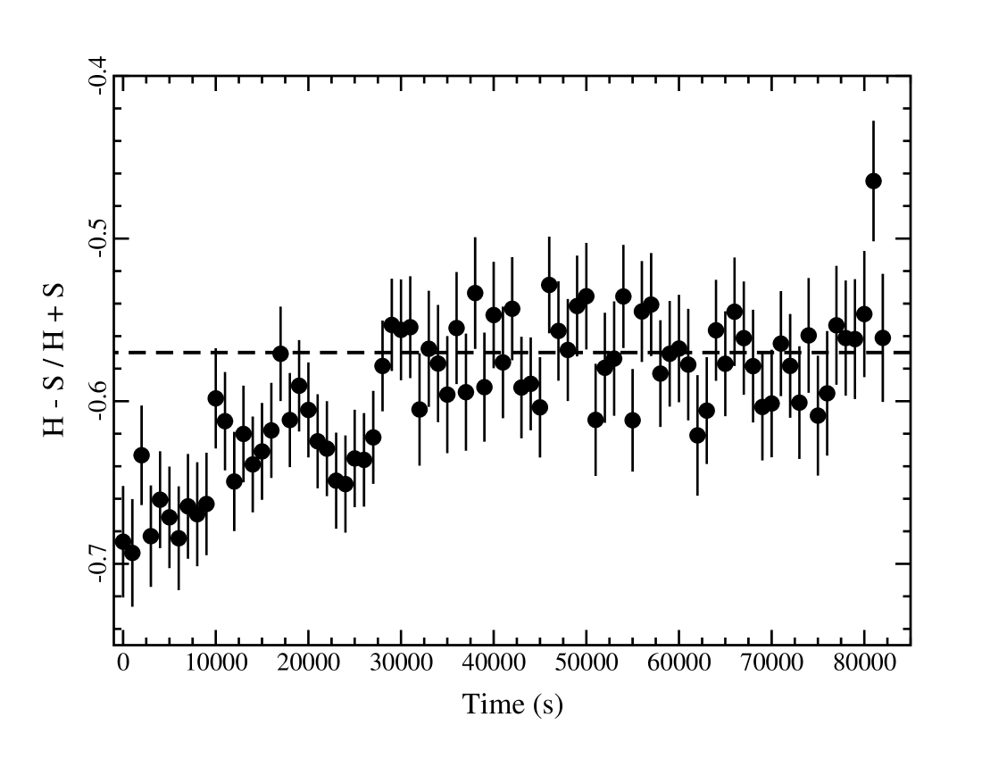
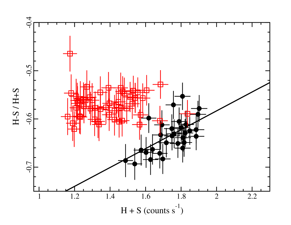
Figure 2: Left panel: A typical hardness-ratio variability curve when comparing low- and high-energy bands. In this case $H=2.5-12{\rm\thinspace keV}$ and $S=0.5-1{\rm\thinspace keV}$. The dashed line marks the average hardness ratio after $30{\rm\thinspace ks}$, the time corresponding to the approximate onset of the flux dip in the light curve. There is spectral variability (spectral hardening) prior to this time, but negligible spectral variability afterwards. Right panel: Hardness ratio as a function of count rate. The data prior to the dip in the light curve (black dots) show a correlation between hardness ratio and count rate (shown by the best-fit solid line). The data after the flux dip (red squares) show no flux dependency.

Likewise prior to the dip (Segment A), the spectral variability showed flux dependency (spectral hardening with increasing count rate; right panel of Fig. 2), which was not evident after the dip.

3.2 Flux-flux analysis

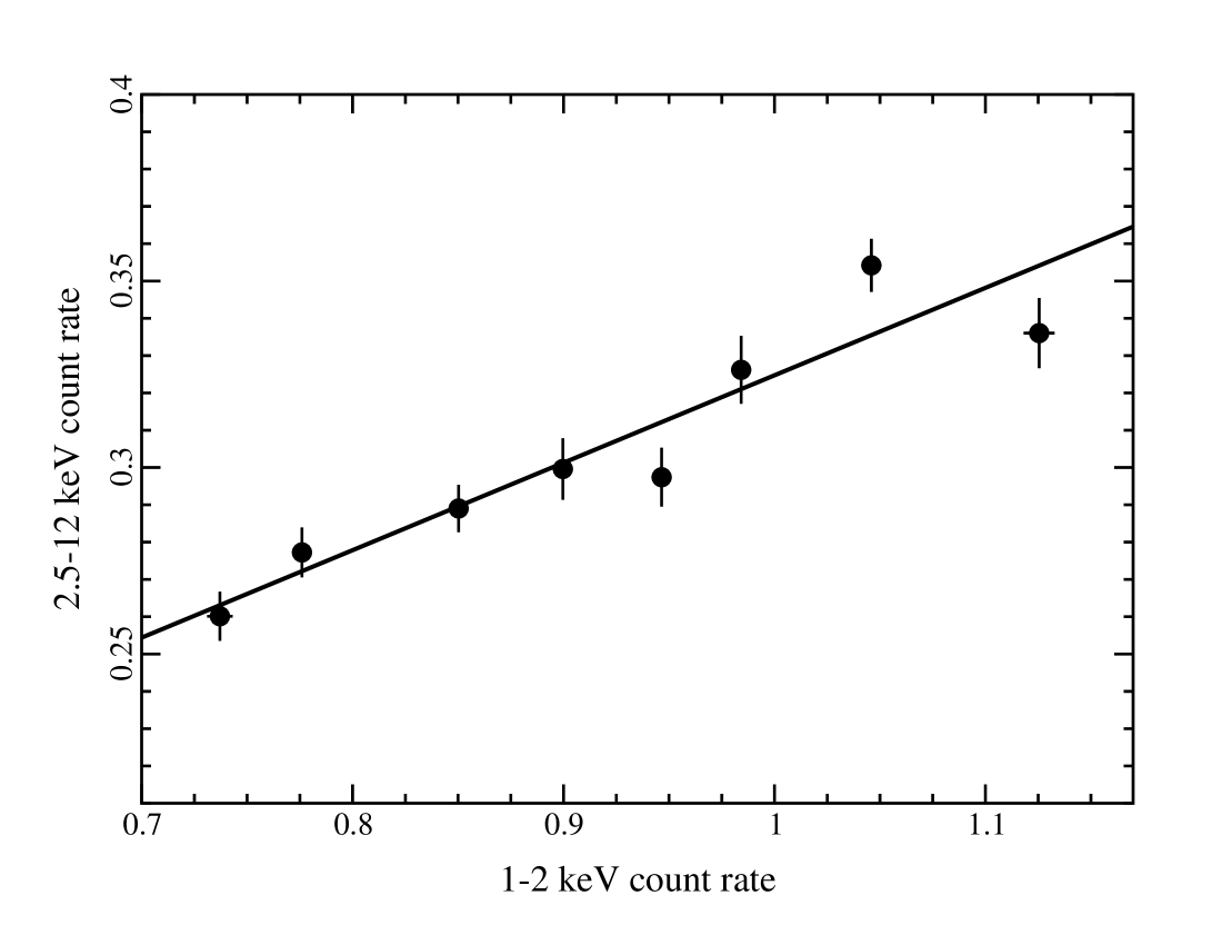
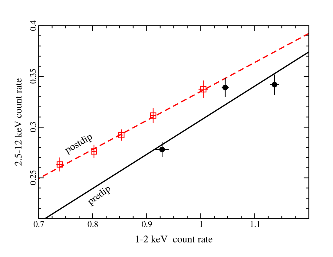
Figure 3: Binned flux-flux plots during 2005. Left panel: The data from the entire observation are not represented well with a linear fit ($\chi^{2}_{\nu}=1.91$). Right panel: Creating a flux-flux diagram for the pre- and post-dip data indicates that each data set can be described with a linear fit, but with a different y-intercept before and after the dip.

Analysing the correlation between variations in two energy bands can reveal different modes of variability (e.g. Taylor et al. 2003). For example, if the binned flux-flux plot (ff-plot) (see Taylor et al. for a complete description) can be described with a linear model then the variability can be associated with variations in the normalisation of a spectral component with a constant shape.

An ff-plot constructed from the 2005 observation is shown in Fig. 3 (left panel). The plot itself was binned as described in Taylor et al. (2003) to overcome intrinsic scatter in the correlation between the two energy bands. A linear fit to the data is statistically unacceptable ($\chi^{2}_{\nu}=1.91$). However, when the ff-plot for the pre- and post-dip data are considered separately the fitting results differ (right panel Fig. 3). In this case, a line adequately fits the data from both time domains. The data in the pre-dip phase are obviously limited so the linear fit is not unique; however what is important is that the relation between the two bands is different (i.e. different y-intercept) during the two phases indicating that the shape and mode of variability is different before and after the flux dip.

Has this behaviour been seen in I Zw 1 before? Fig. 9 in G02 suggests this may be true as the spectrum of I Zw 1 appears softer after the hard X-ray flare. An ff-plot was created from the 2002 data and is presented in Fig. 4. As the observation was short ($\sim 20{\rm\thinspace ks}$), the ff-plot is not binned as was done in the 2005 analysis (Fig. 3). What has been done here, is that a linear relation has been calculated for the data prior to and after the aforementioned hard X-ray flare. The linear relation prior to the flare ($y=-0.824+0.609x$) is slightly different than the relation after the flare ($y=-0.576+0.535x$). Though not highly significant on statistical grounds, the trend in the behaviour seen in 2002 is consistent with that seen in 2005. That is, “dramatic” events in the light curve are consequences of, or actuate, changes in spectral behaviour.

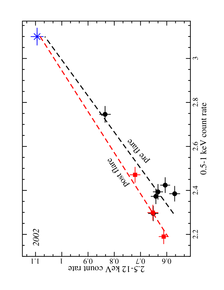
Figure 4: A flux-flux relation during the short 2002 observation. The plot is not binned due to limited data. The dashed-lines identify the best-fit linear relation to the pre- and post-flare data (as identified in the plot). The apparent evolution is similar to that seen in 2005 (Fig. 3).

3.3 Flux-dependent variability

The fractional variability amplitude (e.g. Edelson et al. 2002) was measured in each $5{\rm\thinspace ks}$ block and plotted against the corresponding $2.5-12{\rm\thinspace keV}$ count rate (Fig. 5).

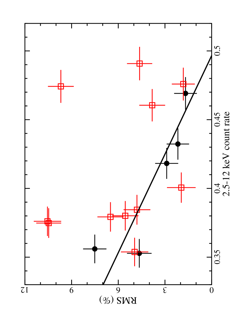
Figure 5: The average fractional variability amplitude in each $5{\rm\thinspace ks}$ block is plotted against the corresponding $2.5-12{\rm\thinspace keV}$ count rate. An anti-correlation in the pre-dip data (black dots) is apparent while the post-dip data (open squares) are scattered.

Over the course of the entire observation there is no relation between the two parameters, but if one considers the pre- and post-dip data separately there does appear to be an anti-correlation between count rate and fractional variability prior to the dip. Fig. 5 is shown for illustration of the potential difference prior to and after the dip. On its own the possible difference in the behaviour is not significant, but it appears interesting in conjunction with other lines of evidence presented in this section.

3.4 Time-resolved spectral fits

To this point the dual-mode spectral variability has been presented in a completely model-independent manner, utilising only count rates and ratios to examine spectral differences. Here we examine the variability further by applying simple models.

The $2-10{\rm\thinspace keV}$ band is dominated by a power law with an average photon index of $\Gamma\approx 2.15$ (G07). Between $6-7{\rm\thinspace keV}$ a broad feature was detected, which is apparently variable in flux but not in energy or width (G07). Each $5{\rm\thinspace ks}$ block was modelled with a single power law in the $2-10{\rm\thinspace keV}$ band while excluding the $5.9-7.1{\rm\thinspace keV}$ range. The fits were statistically acceptable in all cases (i.e. $\chi^{2}_{\nu}\approx 1$), and the photon index in each block was recorded and plotted (Fig. 6).

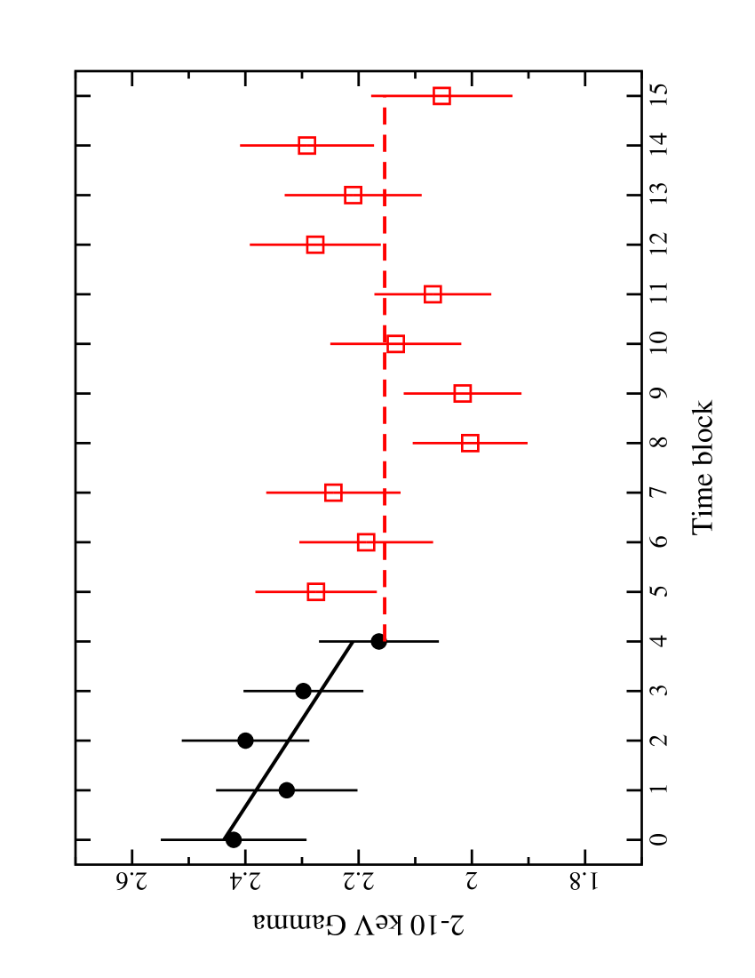
Figure 6: The photon index as measured when fitting the $2-10{\rm\thinspace keV}$ spectrum in each block with a power law (excluding the $5.9-7.1{\rm\thinspace keV}$ band) The abscissa shows the block number. The corresponding start time of each block can be obtained by multiplying the block number by $5000{\rm\thinspace s}$. The best-fit lines to the pre-dip (solid line) and post-dip (dashed line) indicate spectral hardening in the pre-dip stage and a constant photon index in the post-dip.

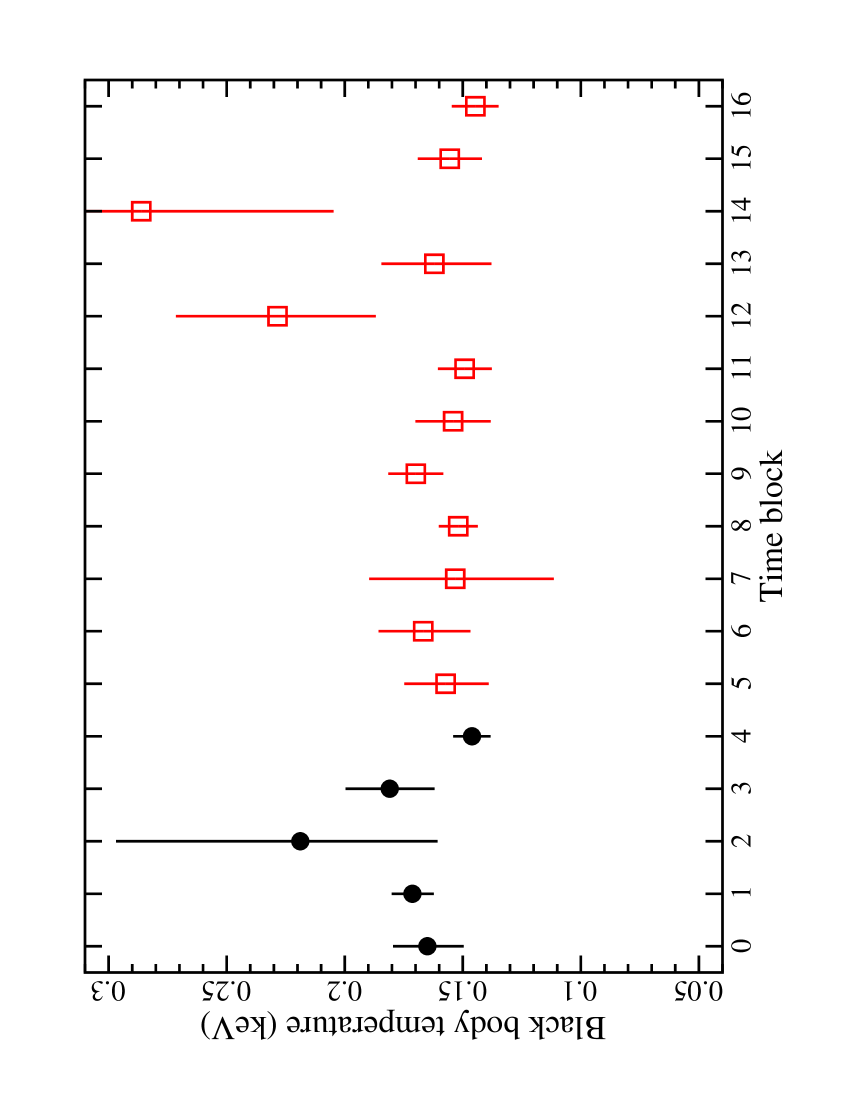
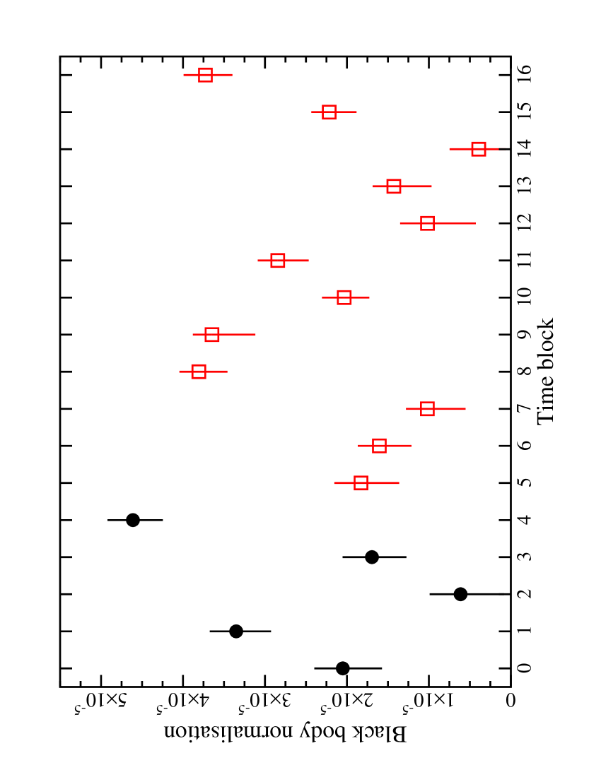
Figure 7: A blackbody plus power law model (modified by constant neutral and ionised absorption, see G07) is applied to each $5{\rm\thinspace ks}$ block to examine variability in the second continuum component. The shape of the second component (i.e. the blackbody temperature in this case) appears constant throughout the observation (top panel). On the other hand, the normalisation of the component seems variable (lower panel). The abscissa is the block number and is described in the text and in Fig. 6.

The average photon index is steeper during Segment A (pre-dip stage) and appears to flatten with time. The best fits to the pre-dip and post-data data clearly support this claim as the post-dip data are consistent with a constant, while the pre-dip fit has a negative slope (spectral hardening). Even though within uncertainties the changes in photon index during the pre-dip phase are modest, the trend in the figure suggests pivot-like behaviour of the power law. The changes in the spectral shape could explain the difficulties encountered by G07 in fitting the average high-energy spectrum with a single power law.

G07 demonstrated that a second low-energy component was necessary to fit the broad-band continuum of I Zw 1, though its origin was unclear. To examine if this second component varied the $2-10{\rm\thinspace keV}$ power law fit in each block was extrapolated to $0.3{\rm\thinspace keV}$ and a blackbody component was added to the model.

In addition, the broad-band spectra were modified by neutral and ionised absorption, which were constant over the observation, as described in G07 and Costantini et al. (2007). The advantage of using a blackbody rather than a second power law is that the low-energy variability could be examined empirically without altering the fit at high energies. However, in Section 4 we will test the variability using spectral models with a more physical interpretation. In all cases, the additional blackbody component improved the broad-band fit over a single power law. The shape (i.e. temperature) of the blackbody in the pn bandpass did not appear notably variable, but the normalisation did appear to change in an erratic manner (Fig. 7).

4 Modelling energy-dependent spectral variability

A spectrum portraying the degree of variability in different energy bins (i.e. an rms spectrum; e.g. Edelson et al. 2002) can offer insight into the origin of the variations and the nature of the continuum in AGNs and GBHs (e.g. Gilfanov et al. 2003; Fabian et al. 2004; Zdziarski 2005; Gierlinski & Done 2006). On relatively short timescales (those within a typical XMM-Newton observation) the rms spectra of AGN usually have a concave-down shape peaking between $0.8-2{\rm\thinspace keV}$ (e.g. Fabian et al. 2002, Markowitz et al. 2006). The most extreme shapes, in terms of amplitude range, are usually seen in NLS1 (e.g. Gallo et al. 2004b,c). However, the rms spectrum of I Zw 1 during the 2002 observation was unlike these, and it even displayed different shapes depending on whether the aforementioned hard X-ray flare was included in the calculation or not (see figure 6 of G02).

To ensure that the Poissonian noise was negligible compared to the rms value, the 2005 rms spectrum was constructed with at least $400$ counts in each energy band and with light curves in $1000{\rm\thinspace s}$ bins. Consequently, the uncertainties were calculated following Ponti et al. (2004). The average rms spectrum of I Zw 1 at the 2005 epoch (Fig. 8 left panel) is unlike the one seen in 2002. This time, the amplitude of the variations tends to increase toward lower energies.

As the rms spectrum in 2002 appeared to vary within the observation (i.e. it exhibited non-stationary behaviour), we searched for similar behaviour in 2005. An rms spectrum was created for each segment (A–D) labeled in Fig. 1. The duration of each segment was approximately $20{\rm\thinspace ks}$ and thus they could be compared to each other. Similar to the 2002 observation the rms spectra in the different segments appear different in shape (Fig. 8 right panel). In particular, the spectrum in Segment A is significantly different than in the other time-segments, which are not completely dissimilar.

In establishing a potential model for the rms spectrum in Fig. 8 we are provided with insight from Section 3.4. What we learned there was that of the two continuum components that make up the average spectrum both vary in normalisation. However, only the power law component varies in shape and only during the pre-dip phase.

We considered first a double power law model, found to fit the average spectrum in G07 reasonably well. This could be interpreted as due to multiple coronae or a continuous, multi-zone corona where both power laws are produced by inverse Compton scattering of low-energy photons. If the time lag between energy bands reported in G07 indicates physical separation of these coronae, then the harder power law is produced in a corona that is more distant from the seed photons (e.g. the accretion disc) than the corona producing the softer power law. Consequently, we assumed that the shape of the harder power law remained constant over the observation, but the normalisation was allowed to vary. The softer power law component was permitted to vary in normalisation throughout the observation, but its photon index was only free to vary during Segment A. The spectrum in each block was fitted with this model accordingly, and the predicted rms spectrum was constructed (plotted over the observed rms spectrum in Fig. 8). The rms spectrum is fitted well between $0.5-4{\rm\thinspace keV}$, but the model predicts considerably more variability at higher and lower energies than is actually observed.

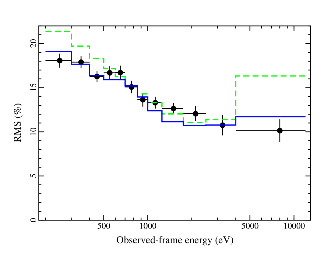
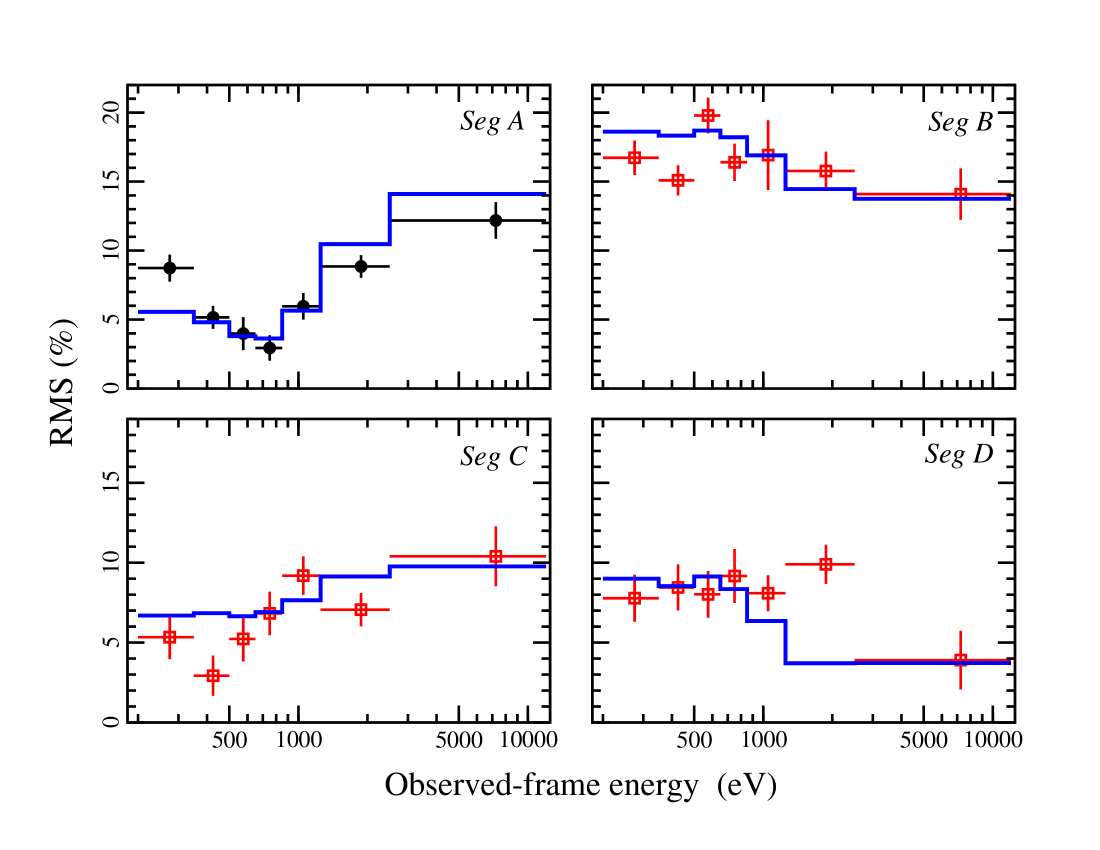
Figure 8: Left panel: The average rms spectrum over the entire observation (black circles). The dashed curve is a simulation of the rms spectrum assuming the spectrum of I Zw 1 is described by a double power law. The solid line is a simulation of the rms spectrum assuming the spectrum is described by a blurred ionised reflector (see Sect. 4 for details). Right panel: An rms spectrum is calculated for each $\sim 20{\rm\thinspace ks}$ segment as indicated in the top right of each panel. The spectrum appears distinctly different in Segment A compared to the other three segments. The solid curve is a simulation of the spectra assuming the blurred ionised reflector model in each segment (see Sect. 4 for details).

A blurred ionised reflection model was also fitted to the average spectrum in G07. While statistically the fit was not as good as the double power law model, it had the advantages of describing the origin of the Fe K$\alpha$ emission line and explaining the long-term (yearly) variability in a self-consistent manner. In adopting this spectral model for the rms simulation, the shape of the reflection component was kept constant throughout, but the normalisation was allowed to vary. Similarly the intrinsic power law was permitted to vary in normalisation, but during the pre-dip phase its slope ($\Gamma$) was also variable. This model produces a very good description of the average rms spectrum (left panel, Fig. 8), with no significant discrepancies over a decade of energy. As this model provided a good description of the average rms spectrum, we also applied it to the rms spectra in the four segments. The rms spectrum in each segment was modelled in the same way as the average rms spectrum. The normalisations of both continuum components were variable in all four segments, and the photon index of the intrinsic power law was variable only in Segment A. Interestingly, this same model fits all four segments relatively well; in particular it describes the differences in Segment A compared to the other segments in a self-consistent manner (right panel, Fig. 8).

Perhaps one advantage of the blurred reflection model is that its spectral variability can be predicted to some degree. In the light-bending scenario the reflection component and illuminating power law continuum vary in a particular way depending on the relative contribution of the two components to the total spectrum (Miniutti & Fabian 2004). As such it is of interest to examine how the two components vary with respect to each other.

For each block, the $0.3-10{\rm\thinspace keV}$ flux of the reflection component was plotted against the flux of the power law component (Fig. 9).

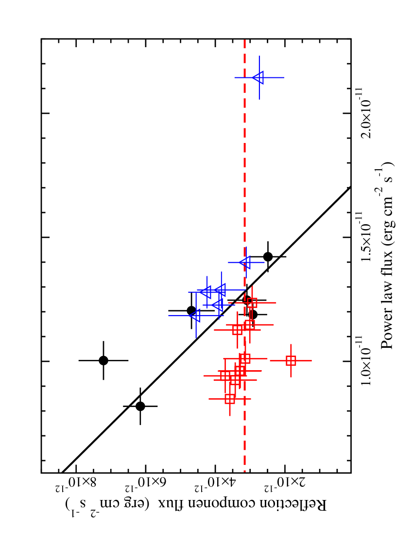
Figure 9: The fluxes of the reflection and power law components in the $0.3-10{\rm\thinspace keV}$ band are plotted against each other. The pre-dip data (black circles) support an anti-correlation in the relation. Post-dip (open red squares) the reflection component is constant despite continued fluctuations in the power law. Block 5, which corresponds to the data at the onset of the dip ( the first block of Segment B), is shown as a black circle in this figure ($x,y=1.0\times 10^{-11},7.2\times 10^{-12}$) as the behaviour is consistent with the Segment A data. For comparison the 2002 data, when I Zw 1 was in a higher flux state, are shown as well (blue triangles). The relation in 2002 appear more comparable to the pre-dip relation in 2005 than to the post-dip relation.

As has been demonstrated regularly throughout this work the pre-dip flux-flux relation is different from the post-dip relation. The pre-dip data show a clear anti-correlation between the power law and reflection flux. Whereas in the post-dip data, the reflection component appears constant despite continued variations in the power law. The different relations indicate that there is a change in the mode of variability after the dip.

For comparison the data from fitting the 2002 observation in a similar way have been plotted as well (open triangles in Fig. 9). In 2002, when I Zw 1 was in a higher flux and more power law dominated state, the flux-flux relation exhibits a negative slope and is more consistent with the pre-dip behaviour in 2005 (i.e. fluxes are anti-correlated). The exception is during the 2002 flare when the single data point from that time fell on the relation showing no correlation between the fluxes (i.e. the post-dip relation). This indicates that the relative amount of reflected flux increased during that time, which is in complete agreement with the intensified ‘red-wing’ emission identified in figure 12 and 13 of G07. This is consistent with the possibility that the power law emission during the flare arises from a region physically distinct (e.g. closer to the black hole) from the “typical” emitter.

5 Discussion

5.1 State transitions in accreting black holes

The 2005 observation of I Zw 1 reveals two distinct modes of spectral variability. The variability in the first $\sim 30{\rm\thinspace ks}$ can be described with changes in normalisation and shape (specifically $\Gamma$) of the spectral components, while the variability in the remaining data is attributed to fluctuations in normalisation alone.

Particularly curious is that the time when the AGN makes the transition from one mode of spectral variability to the other is associated with the occurrence of a flux dip in the broad-band light curve. To the best of our knowledge, this is the first report of such “marking” of a mode change in an AGN. The marking of a change in spectral behaviour with a notable event in the light curve may not be unique to this observation of I Zw 1. Examination of the flux-flux relation during the short 2002 XMM-Newton observation (Fig. 4), along with figure 9 of G04, suggest that the spectral change there is coincident with the modest X-ray flare.

Such state transitions, bimodal spectral variability, and flux dips and flares are commonly seen in GBHs (e.g. Fender & Belloni 2004; Remillard & McClintock 2006; Malzac et al. 2006). In addition, the behaviour shown in the right panel of Fig. 2 is similar to that found during state changes and oscillations in the very high state of GBHs. However, the rapidity of the change argues that it is unlikely to be due to changes in the disc itself, but more likely related to the magnetic structure above the disc and could be connected with the existence of a jet.

5.2 A jet-like nature of the corona in I Zw 1?

The broad iron lines observed in the 2002 and 2005 spectra of I Zw 1 are very similar in appearance and were likely emitted several tens of ${\thinspace r_{\rm g}}$ from the central black hole (G07). Since there were no obvious time delays between the continuum and reflection component it is reasonable to assume the illuminating corona occupies a similar spatial region as the reflection component. This suggests that at least some of the hot, optically thin plasma blankets several tens of ${\thinspace r_{\rm g}}$ of the accretion disc and is responsible for the mean X-ray properties exhibited by I Zw 1.

There is also evidence indicating that the hard X-ray flare observed in the 2002 data originated much closer to the black hole since the reflection spectrum during the flare appeared to be redshifted much more than the average broad line (G07). This suggests that there is a second component to the corona that is more compact and centrally located perhaps in a jet-like geometry. This jet component is responsible for the rapid events seen in I Zw 1 (e.g. flux flares and dips), illuminating the inner accretion disc, and replenishing the more diffuse corona. I Zw 1 is comparatively radio quiet. The radio source in I Zw 1 has a steep spectrum, perhaps indicative of optically thin synchrotron emission, and is unresolved with a physical size $\leq 0.38{\rm\thinspace kpc}$ (Kukula et al. 1998). The implied compactness of this proposed jet is consistent with the aborted-jet model proposed for radio-quiet AGN (Ghisellini et al. 2004).

The jet component could account for the pre-dip behaviour in I Zw 1. High-energy particles could be expelled via the jet, their spectrum hardening as they propagate further from the accretion disc and source of low-energy seed photons. The dip itself could correspond to an interval when this ejected component dims below the average coronal flux (i.e. that of the extended corona). The scenario is not unlike that suggested to describe the connection between superluminal radio flares and soft X-ray flux dips in the GBH GRS 1915+105 (Vadawale et al. 2003).

The 2002 observation of I Zw 1 when a hard X-ray flare was detected (G04) is plausibly consistent with this jet picture. In that case, the ejected material may have collided with more material in its path resulting in a shock and consequent flare, which then illuminated the inner accretion disc resulting in intensified reflected emission.

While the aborted-jet model and variations along that line (e.g. Henri & Petrucci 1997, Malzac et al. 1998) can qualitatively describe our X-ray observations of I Zw 1, they are not unique explanations. The compact hot plasma envisioned in I Zw 1 could be attributed to magnetic flares atop the accretion disc (i.e. an active corona) (e.g. Beloborodov 1999a), which could produce similar behaviour. There are distinctions between these two models, some of which may be identified with future observations.

The jet model places the compact source on the spin axis of a Kerr black hole, thus preferentially illuminating the inner accretion disc. Such conditions would generate extremely redshifted iron emission, similar to that seen by Wilms et al. (2001) in MCG–6-30-15. The increased photon-collection ability proposed for future X-ray missions can reveal such emission lines in dimmer AGN. In contrast, there is no propensity for the active-corona model to produce highly redshifted reflection features as emission would originate at different disc-radii. In fact, Beloborodov (1999a) suggests that if the flaring plasma is composed of $e^{\pm}$ then it should be accelerated $away$ from the disc at mildly relativistic velocities ($v/c\approx 0.1-0.7$) by radiation pressure. This would likely yield weaker reflection features and if the outflow is optically thick, the effect would be compounded as emission from the accretion disc would be obscured (Beloborodov 1999b). Moreover, an optically thick $e^{\pm}$ wind produces a shifted and smeared annihilation feature at $E>511{\rm\thinspace keV}$ (Beloborodov 1998), perhaps detectable with future gamma-ray detectors. The feature has not been detected in the spectra of AGNs or GBHs with jets, and its presence depends on the composition of the jet.

Even though the escape velocity is not exceeded in the aborted-jet model, high velocities can still be achieved. The escape velocities from a Kerr black hole are $0.9c$ and $0.7c$ at $2{\thinspace r_{\rm g}}$ and $4{\thinspace r_{\rm g}}$, respectively (see equation 3 of Ghisellini et al. 2004). The velocities can be much higher than what is predicted with the active-corona model. VLBI imaging has revealed sub-pc scale jets in several radio-quiet Seyfert galaxies (e.g. Ulvestad 2003). It is conceivable that with improvements in interferometry and imaging techniques (see Ulvestad 2003 and references therein) proper motions on even smaller scales can be measured.

The radiation scattered by the mildly relativistic wind in the active-corona model will have polarisation parallel to the disc normal, which may be noticeable in polarimetry observations. On the other hand, beamed radiation from the jet exhibits polarisation perpendicular to the jet. Furthermore, the X-ray emission reflected from an accretion disc will be polarised with angle and degree depending on conditions in the gravitational field, and can elucidate the geometry of the illuminating source (e.g. Dovčiak, Karas & Matt 2004). This bolsters the demand for a sensitive polarimeter on future X-ray mission such as the X-Ray Evolving Universe Spectrometer ($XEUS$).

5.3 On the blurred reflection interpretation

The presence of a short jet above the black-hole and accretion-disc system provides a possible description for the illuminating source in the light-bending model illustrated by Miniutti & Fabian (2004). In that model the accreting black hole exists in three distinct temporal states depending on how distant the primary continuum source (e.g. the jet) is from the black hole. In the low-flux case (regime I), the compact continuum source is within a few ${\thinspace r_{\rm g}}$ of the black hole, and the observed spectrum is reflection dominated. In this case the variability of the reflection and continuum components are correlated. As the distance of the continuum source grows the AGN brightens and enters regime II. Here the variability of the reflection component reaches a minimum and appears to show no correlation with the continuum changes. The behaviour is very similar to what we see in the post-dip state in Fig. 9. As the distance of the continuum continues to increase (e.g. $\mathrel{\hbox{\hbox to0.0pt{\hbox{\lower 4.0pt\hbox{$\sim$}}\hss}\hbox{$>$}}}20{\thinspace r_{\rm g}}$) the AGN enters a high-flux state and regime III. In this state general relativistic effects are minimal, and the reflection and continuum fluxes are anti-correlated. The predicted behaviour is similar to what is seen in the pre-dip state (and possibly during the high-flux 2002 observation) (Fig. 9).

Is the apparent change in behaviour marked by the flux dip in the light curve a transition of the black hole from regime III to II? While the behaviour is consistent, the luminosity of the continuum prior to and after the dip is not substantially different as would be expected in the light-bending scenario. In addition the continuum shape appears to be changing during the pre-dip phase. This would indicate that if we consider the light-bending scenario to describe the observed behaviour we must allow the compact continuum source to undergo intrinsic changes. This is not an unreasonable requirement. If the emission process in the continuum source is Comptonisation then one would expect that when the distance of the hot plasma (i.e. corona) from the seed photons changes so to does the shape of the emitted spectrum. Specifically as the distance of the corona from the seed photons increases the emitted power law spectrum flattens.

6 Conclusions

The short-term spectral variability of I Zw 1 as observed in an $85{\rm\thinspace ks}$ XMM-Newton observation is discussed in detail. The behaviour in the spectral variability is temporally distinct and marked by a dip in the broad-band count rate at $\sim 30{\rm\thinspace ks}$ into the observation. Prior to the dip the variability requires changes in shape and normalisation of the spectral components. Only changes in normalisation are required after the dip. The changes occur on dynamically short timescales and likely would not be observable in GBHs.

The ionised reflection model is applied to the temporal data with good agreement. The interpretation can follow the light-bending scenario, but requires intrinsic changes in the shape of the primary continuum source prior to the dip. If we consider the corona to be the base of a possible jet then the spectral changes could arise from material that is expelled from it. The aborted jet scenario seems consistent with the 2002 and 2005 observations of I Zw 1, which possesses parallels with some GBH observations.

References

- [1] Belloni T., Mendez M., King A. R., van der Klis M., van Paradijs J., 1997, ApJ, 479, L145
- [2] Beloborodov A. M., 1998, ApJ, 496, L105
- [3] Beloborodov A. M., 1999a, ApJ, 510, L123
- [4] Beloborodov A. M., 1999b, MNRAS, 305, 181
- [5] Boller Th., Brandt W. N., Fabian A. C., Fink H. H., 1997, MNRAS, 289, 393
- [6] Brandt W. N., Boller Th., Fabian A. C., Ruszkowski M. 1999, MNRAS, 303, L58
- [7] Costantini E., Gallo L. C., Brandt W. N., Fabian A. C., Boller Th., 2007, accepted by MNRAS (astro-ph/0702553)
- [8] Dovčiak M., Karas V., Matt G., 2004, MNRAS, 355, 1005
- [9] Edelson R., Turner T. J., Pounds K., Vaughan S. Markowitz A., Marshall H., Dobbie P., Warwick R., 2002, ApJ, 568, 610
- [10] Esin A. A., Narayan R., Cui W., Grove J. E., Zhang S., 1998, ApJ, 505, 854
- [11] Fabian A. C. et al. , 2002, MNRAS, 335, L1
- [12] Fabian A. C., Miniutti G., Gallo L., Boller Th., Tanaka Y., Vaughan S., Ross R. R., 2004, MNRAS, 353, 1071
- [13] Fender R., Belloni T., 2004, ARA&A, 42, 317
- [14] Gallo E., Fender R. P., Pooley G. G., 2003, MNRAS, 344, 60
- [15] Gallo L. C., Boller Th., Brandt W. N., Fabian A. C., Vaughan S., 2004a, A&A, 417, 29 (G04)
- [16] Gallo L. C., Boller Th., Tanaka Y., Fabian A. C., Brandt W. N., Welsh W. F., Anabuki N., Haba Y., 2004b, MNRAS, 347, 269
- [17] Gallo L. C., Tanaka Y., Boller Th., Fabian A. C., Vaughan S., Brandt W. N., 2004c, MNRAS, 353, 1064
- [18] Gallo L. C., Brandt W. N., Costantini E. Fabian A. C., Iwasawa K., Papadakis I. E., 2007, accepted by MNRAS (astro-ph/0610283) (G07)
- [19] Gierlinski M., Done C., 2006, MNRAS, 371, 16
- [20] Gilfanov M., Revnivtsev M., Molkov S., 2003, A&A, 410, 217
- [21] Greiner J., Morgan E. H., Remillard R. A., 1996, ApJ, 473, L107
- [22] Ghisellini G., Haardt F., Matt G., 2004, A&A, 413, 535
- [23] Henri G., Petrucci P. O., 1997, A&A, 326, 87
- [24] Jansen F. et al. 2001, A&A, 365, L1
- [25] Malzac J. G. et al. , 2006, A&A, 448, 1125
- [26] Malzac J., Jourdain E., Petrucci P. O., Henri G., 1998, A&A, 336, 807
- [27] Markoff S., Falcke H., Fender R., 2001, A&A, 372, L25
- [28] Markowitz A., Papadakis I. E., Arevalo P., Turner T. J., Miller L., Reeves J. N., 2006, ApJ accepted (astro-ph/0611072)
- [29] McClintock J. E., Remillard R. A., 2006, in Lewin W. H. G., van der Klis M., eds, Compact Stellar X-Ray Sources. Cambridge Univ. Press, (astro-ph/0306213)
- [30] McHardy I. M., Koerding E., Knigge C., Uttley P., Fender R. P., 2006, Nature, 444, 730
- [31] Merloni A., Heinz S., di Matteo T., 2003, MNRAS, 345, 1057
- [32] Miller J. M., Homan J., Steeghs D., Rupen M., Hunstead R. W., Wijnands R., Charles P. A., Fabian A. C., 2006, ApJ, 653, 525
- [33] Miniutti G., Fabian A. C., 2004, MNRAS, 349, 1435
- [34] Ponti G., Cappi M., Dadina M., Malaguti G., 2004, A&A, 417, 451
- [35] Kukula M. J., Dunlop J. S., Hughes D. H., Rawlings S., 1998, MNRAS, 297, 366
- [36] Remillard R. A., McClintock J. E., 2006, ARA&A, 44, 49
- [37] Shakura N. I., Sunyaev R. A., 1973, A&A, 24, 337
- [38] Taylor R., Uttley P., McHardy I., 2003, MNRAS, 342, 31
- [39] Ulvestad J. S., 2003, in Zensus J. A., Cohen M. H., Ros E., eds, Radio Astronomy at the Fringe. ASP Conf. Series Vol. 300, p97
- [40] Vadawale S. V., Rao A. R., Naik S., Yadav J. S., Ishwara-Chandra C. H., Pramesh Rao A., Pooley G. G., 2003, ApJ, 597, 1023
- [41] Wilms, J., Reynolds C. S., Begelman M. C., Reeves J., Molendi S., Staubert R., Kendziorra E., 2001, MNRAS, 328, L27
- [42] Vestergaard M., Peterson B., 2006, ApJ, 641, 689
- [43] Zdziarski A. A., 2005, MNRAS, 360, 816