Hydrodynamic response of rotationally supported flows in the Small Shearing Box model

The hydrodynamic response of the inviscid small shearing box model of a midplane section of a rotationally supported astrophysical disk is examined. An energy functional ${\cal E}$ is formulated for the general nonlinear problem. It is found that the fate of disturbances is related to the conservation of this quantity which, in turn, depends on the boundary conditions utilized: ${\cal E}$ is conserved for channel boundary conditions while it is not conserved in general for shearing box conditions. Linearized disturbances subject to channel boundary conditions have normal-modes described by Bessel Functions and are qualitatively governed by a quantity $\Sigma$ which is a measure of the ratio between the azimuthal and vertical wavelengths. Inertial oscillations ensue if $\Sigma>1$ - otherwise disturbances must in general be treated as an initial value problem. We reflect upon these results and offer a speculation.

“Extraordinary how mathematics help you to know yourself.”
Samuel Beckett, Molloy

1 Introduction

The hydrodynamic response in small shearing box (SSB hereafter) models of rotationally supported flows has been receiving renewed attention over the past few years. Because such fluid configurations do not support supercritical linear instabilities alternative forms of transition, possibly subcritical, have been proposed, discussed and explored in numerous recent studies (Ioannou & Kakouris, 2001, Longaretti, 2002, Chagelishvilli et al., 2003, Yecko, 2004, Mukhopadhyay et al. 2004, Afshordi et al. 2004, Umurhan & Regev, 2004, Sternberg, 2005, Lesur & Longaretti, 2005, Balbus & Hawley, 2006, Rincon et al. 2007, Ji et al., 2006, Williams, 2006, Jiménez et al., 2006, Shen et al., 2006). The identification of a route to sustained nonlinear activity for three dimensional disturbances has been elusive for flows that are wall-bounded (see recently Rincon et al. 2007) and for flows having open boundaries (Shen et al., 2006) although weak levels of activity have been reported by Lesur & Longaretti (2005) near the Rayleigh line in flows with open boundaries.

Far from answering whether or not such transitions do exist in these flows, we instead identify two clues which could be used to cast some light onto this question in the future. To this end we reconsider the dynamics of inviscid anticylonic Rayleigh stable flows in the SSB model (i.e., rotating plane Couette flow, rpCf hereafter) subject to shearing boundary conditions (Goldreich & Lynden-Bell, 1965, Rogallo, 1981, Knobloch, 1984, Korycansky, 1992, SBC hereafter) or channel boundary conditions (e.g., Yecko, 2004, Mukhopadhyay, et al. 2004, Lesur & Longaretti, 2005, Rincon et al. 2007, CBC hereafter).

The first result is a general nonlinear feature pertaining to the energetics of such flows. If one defines ${\cal E}$ as the total energy of the flow in the SSB, whose dynamical constituent includes the total kinetic energy, (i.e., the energy formed by considering the total velocity - which is to say the velocity fluctuations plus background shear flow), the fate of ${\cal E}$ depends upon the boundary conditions employed. ${\cal E}$ is conserved for (but not limited to) (i) disturbances subject to CBC, (ii) azimuthally and vertically periodic, radially localized disturbances in radially unbounded domains. On the other hand, disturbances subject to SBC do not identically conserve ${\cal E}$ and its temporal quality depends critically upon the dynamics within the domain. The nonconservation of ${\cal E}$ for flows subject to SBC relates to the feature that the kinetic energy of a fluid parcel jumps when it crosses the (quasi) periodic radial boundaries.

For our second result, we find that there are qualitative differences in the behavior of linearized disturbances subject to CBC depending on whether or not the quantity $\Sigma$ is less than or greater than 1. This parameter is defined as

$$\Sigma=4\frac{2(2-q)}{q^{2}}\frac{\ell_{y}^{2}}{\ell_{z}^{2}},$$ (1)

where $\ell_{z},\ell_{y}$ are the disturbance length scales in the vertical (like the disk normal) and streamwise (like the disk azimuth) directions of any given modal disturbance. The global flow for which the SSB is meant to represent is characterized by a rotation rate $\Omega$ that depends on the radial coordinate $R$ according to the relationship $\Omega\propto R^{-q}$. This means that on the local scale there is a Couette velocity profile given as $U=-q\Omega_{0}x{\bf{\hat{y}}}$. Keplerian flow is when $q=3/2$. Additionally and hereafter, we will consider linear shear profiles that are anti-cyclonic, i.e., those in which $q>0$. At infinite Reynolds numbers (Re $=\infty$) axisymmetric linear instability (Taylor vortices) occurs for $q\geq 2$. The significance of $\Sigma$ was recognized in previous studies (Knobloch, 1984, Korycansky, 1992, Sternberg, 2005, as the parameter $\beta$ in Balbus & Hawley, 2006) of disturbances subject to SBC. In those studies it was demonstrated that modes always decay. If the mode was initially leading then it will experience one maximum whereas if the mode is trailing it never experiences a maximum. However, irrespective of this the asymptotic decay of disturbances depends on $\Sigma$: for $\Sigma<1$ the decay is monotonic while for $\Sigma>1$ the decay oscillatory.

In flows subject to CBC, with given vertical and azimuthal wavenumbers, if $\Sigma>1$ the system supports a countably infinite number of inertial normal modes described by Bessel Functions oscillating without growth or decay. Otherwise if $\Sigma<1$ the system allows for only one eigenmode - meaning that in general the dynamical response cannot be characterized by discrete normal modes - in which case, such linearized disturbances must be treated as an initial value problem, a situation well-known in studies of plane-Couette flow (Schmid & Henningson, 2000, pCf hereafter).

We would like to note that the two main results we report upon here may be clues in explaining the results of Lesur & Longaretti (2005) who show that there is a subcritical transition beyond the Rayleigh line in rpCf when SBC conditions are applied whereas no such transition was observed for such flows under CBC boundary conditions. On a related note, as well, Lithwick (2007) demonstrated the existence of steady vortex structures in 3D rpCf flow for Keplerian shear profiles when SBC are applied. We return to this in the discussion.

2 Equations, Boundary Conditions and Two Integral Statements

The equations we consider represent the dynamics taking place in a “small-shearing box” section located at a cylindrical radius $R=R_{0}$ centered about the midplane of a disk rotating about a central object with the local rotation vector, $\Omega_{0}{{\bf\hat{z}}}$. With the external gravity set to zero and the density constant, these non-dimensionalized equations (Goldreich & Lynden-Bell, 1965,Umurhan & Regev, 2004) are

$$\nabla\cdot{\bf u}=0,$$ (2)

$$(\partial_{t}-q\Omega_{0}x\partial_{y})u+{\bf u}\cdot\nabla u-2\Omega_{0}v=-{\partial_{x}P}$$ (3)

$$(\partial_{t}-q\Omega_{0}x\partial_{y})v+{\bf u}\cdot\nabla u+(2-q)\Omega_{0}u=-{\partial_{y}P},$$ (4)

$$(\partial_{t}-q\Omega_{0}x\partial_{y})w+{\bf u}\cdot\nabla w=-{\partial_{z}P}.$$ (5)

The flow on these scales is equivalently known as incompressible rpCf (e.g., Nagata, 1986, Yecko, 2004). In this form these equations are the inviscid limit of those considered by Longaretti (2002), Mukhopadyay et al. (2005) and Yecko (2004). In the language of this paper, $x$ corresponds to the radial (shearwise) coordinate, $y$ corresponds to the azimuthal (streamwise) coordinate and $z$ corresponds to the vertical (spanwise) coordinate - with the corresponding velocity disturbances ${\bf u}=\{u,v,w\}$. These velocities represent deviations over the steady Keplerian flow (as manifesting itself in this rotating frame) given by $-q\Omega_{0}x{\bf{\hat{y}}}$. $\Omega_{0}$ is sometimes also referred to as the Coriolis parameter, and in these nondimensionalized units $\Omega_{0}$ is $1$. The local shear gradient is defined as the exponent of the general rotation law $\Omega(R)=\Omega_{0}(R/R_{0})^{-q}$.

Boundary Conditions. We first present and discuss the means by which one administers shearing boundary conditions (SBC) in the SSB. By this we mean to say that the flow variables $\bf u$, and $p$ are (a) periodic in the azimuthal and vertical directions on scales $L_{y}=1$ and $L_{z}=1$ respectively and (b) are simply periodic (on scale $L_{x}=1$) in the shearwise (radial) direction with respect to a coordinate frame that moves with the local shear (e.g. Lynden-Bell & Goldreich, 1965, Rogallo, 1981). In this work we refer to this coordinate frame as the shearing coordinate frame (SC for short). The coordinate frame of an observer in the rotating frame, will be referred to as the non-shearing coordinate frame (NSC for short). In this sense the fundamental equations (2-5) have been expressed in the NSC frame.

If $(X,Y,Z,T)$ represent the independent variables in the SC frame then we say they are related to the NSC variables by $X=x,\ Y=y+q\Omega_{0}xt,\ Z=z,\ T=t.$ If $f$ is any dynamical quantity then in the SC frame the periodic boundary conditions in the shearwise, azimuthal and vertical directions respectively are $f(X,Y,Z)=f(X+L_{x},Y,Z),\ f(X,Y,Z)=f(X,Y+L_{y},Z),\ f(X,Y,Z)=f(X,Y,Z+L_{z}).$ Of course this means in general that $f(X,Y,Z)=f(X+L_{x},Y+L_{y},Z+L_{z})$. As expressed in the NSC frame, the periodicity in the azimuthal and vertical directions appears like $f(x,y,z)=f(x,y+L_{y},z),\ f(x,y,z)=f(x,y,z+L_{z}),$ while the periodicity in the shearwise direction is $f(x,y,z)=f(x+L_{x},y+q\Omega_{0}tL_{x},z).$ Because of the periodicity in the azimuthal direction this statement takes the form $f(x,y,z)=f(x+L_{x},y+\tilde{y},z)$ where $\tilde{y}(t)=q\Omega_{0}tL_{x}({\rm mod}\ L_{y})$. Note that this means that only after exactly integer values of $q\Omega_{0}tL_{x}/L_{y}$, (i.e., when $\tilde{y}=0$) are the SC and NSC frames coincident, meaning every $T_{{\rm rep}}=L_{y}/q\Omega_{0}L_{x},$ time units. Evidentally the SBC are time dependent when viewed by an observer in the NSC frame.

When enforcing channel boundary conditions (CBC) on (2-5) we require that all quantities are periodic in the vertical and azimuthal directions (in the NSC frame) while requiring no normal-flow at the channel boundaries. This latter statement amounts to $u=0$ at $x=0,L_{x}$.

A Pair of Integral Statements. The dynamical equations (2-5) describe the evolution of velocities which are disturbances about a steady rotationally supported flow which, on the SSB scales, is the linear shear. Thus, the steady solution, ${\bf u}=0$, is interpreted as the undisturbed state. We now consider the total velocity $\bf v$ defined as ${\bf v}\equiv-q\Omega_{0}x{\bf{\hat{y}}}+\bf u.$ As such the governing equations of motion (2-5) are more concisely written in vector form,

$$\partial_{t}{\bf v}+{\bf v}\cdot\nabla{\bf v} = -\nabla p-2\Omega_{0}{\bf{\hat{z}}}\times({\bf v}+q\Omega_{0}x{\bf{\hat{y}}}),$$ (6)

$$\nabla\cdot{\bf v} = 0.$$ (7)

Note that these equations written in this way have appeared in other works (e.g., Lesur & Longaretti, 2005). Taking the inner product of (6) with ${\bf v}$ and following some manipulation yields the following

$${\partial_{t}}\varepsilon+{\bf v}\cdot\nabla\left(\varepsilon+p\right)=0,\qquad\varepsilon\equiv\frac{{\bf v}^{2}}{2}-q\Omega_{0}^{2}x^{2}.$$ (8)

With use of the incompressibility condition (7) we may integrate (8) over the full spatial domain to find,

$$\frac{d{\cal E}}{dt}=-\int_{{\cal S}}{(\varepsilon+p){\bf v}\cdot{\bf\hat{n}}}dS,\qquad{\cal E}\equiv\int_{{\cal V}}\varepsilon dV,$$ (9)

in which ${\cal V}$ and ${\cal S}$ are the volume and surface-boundaries and ${\bf\hat{n}}$ is the unit normal of the bounding surface. ${\cal E}$ is comprised of (a) the term ${\bf v}^{2}/{2}$ which is the kinetic energy and (b) the potential-like term $-q\Omega_{0}^{2}x^{2}$. The global integral ${\cal E}$ can change due to the influx of $\varepsilon$ across the boundaries , i.e., $\int_{{\cal S}}\varepsilon{\bf v}\cdot{{\bf\hat{n}}}dS$, and through the external work done upon the system denoted by the boundary integral $\int_{{\cal S}}p{\bf v}\cdot{{\bf\hat{n}}}dS$. The appropriate Bernoulli function for this system is $\varepsilon+p$. The functional ${\cal E}$ is analogous to the total energy contained in the flow and its dynamical response (see below) is characterized by the total kinetic energy variations in the box.

By contrast we follow the same procedure as above but consider an energy functional comprised only of the disturbance velocities. Beginning with (3-5) and taking its inner product with the disturbance velocity ${\bf u}$, followed by the use of (2) and either the SBC or CBC boundary conditions, one can integrate over the domain to find

$$\frac{dE}{dt}\equiv\frac{d}{dt}\int_{{\cal V}}\xi dV=q\Omega_{0}\int_{{\cal V}}uvdV;\qquad\xi\equiv\small\mbox{$\frac{1}{2}$}{\bf u}^{2}.$$ (10)

The disturbance energy per unit volume is $\xi$. The total domain integrated disturbance energy is $E\equiv\int_{{\cal V}}\xi dV$. The above is known in more general terms as the Reynolds-Orr equation (e.g. Schmid & Henningson, 2000) and relates the change of the total disturbance energy to the domain integrated correlation between $u$ and $v$. In the absence of shear (i.e., $q=0$), the disturbance energy is conserved.

Inspection of the Reynolds-Orr relationship says that so long as there is some correlation between the radial and azimuthal velocities the disturbance energy must fluctuate in time. However from the definitions of ${\cal E}$ and $E$ we have

$${\cal E}=E+E_{{\rm shear}};\ E_{{\rm shear}}\equiv\int_{{\cal V}}\left[{-q\Omega_{0}xv+\small\mbox{$\frac{1}{2}$}q^{2}\Omega_{0}^{2}x^{2}}\right]dV,$$ (11)

we see that disturbance energy $E$ is related to ${\cal E}$ (the global energy) in an intimate way via $E_{{\rm shear}}$, which we consider to be the disturbance energy affected by the shear in a dynamical sort of way.

To appreciate the significance of these relationships we first apply CBC to (9) and find that

$$\frac{d{\cal E}}{dt}=0.$$ (12)

This means that the fluctuations in $E$ come at the expense of $E_{{\rm shear}}$ in an equal but opposite way throughout the dynamical response of the flow; i.e., the stresses comprising the RHS of (10) is a measure of the time rate of change between these two forms of measured energy.

We note that if instead of the CBC we require that the flow be periodic in $y$ and $z$ (again) but that all flow quantities decay sufficiently fast as $x\rightarrow\pm\infty$, then the boundary term in (9) also vanishes and (12) again follows. The same is true if the vertical domain is unbounded and disturbances are vertically localized as well, i.e. (12) also follows if disturbances similarly decay as $z\rightarrow\pm\infty$.

Matters are less clear when SBC are employed because ${\cal E}$ is no longer conserved, evolving according to ( with boundaries of the periodic box set at $x=\pm\small\mbox{$\frac{1}{2}$}$),

$$\frac{d{\cal E}}{dt}=q\Omega_{0}\int_{{\cal S}_{1}}uvdydz,$$ (13)

in which ${\cal S}_{1/2}$ is the boundary surface at $x=1/2$. In general the right-hand side of (13) is not expected to be zero and it means that ${\cal E}$ can vary with respect to time when SBC are employed. The physical reason for this is clear: as a fluid parcels exits from one radial boundary with a given azimuthal velocity it reenters through the other boundary with an azimuthal velocity boosted by the difference in the background velocities between the two radial boundaries. Another observation about this is that disturbances are forced a-priori to have a correlation scale set by the length of the box $L$ (Regev & Umurhan, 2008). We note that ${\cal E}$ will be conserved for SBC if the disturbances are sufficiently localized in the interior of the computational domain so that there is no power (i.e. fluid motion) near the bounding surface ${\cal S}_{1/2}$ (Nusser, 2007).

3 Linear Analysis with CBC

In considering the response of the flow in the channel model we shall assume initially the general form $f(x,y,z,t)=f_{{}_{\alpha\beta}}(x,t)\exp({i\alpha y+i\beta z})+c.c.$ Linearization of (2-5) followed by introduction of this spatial Fourier form and rearranging results in the single equation for the radial velocity

$$(\partial_{t}-iq\Omega_{0}x\alpha)^{2}(\partial^{2}_{x}-\beta^{2}-\alpha^{2})u_{{}_{\alpha\beta}}=\omega_{e}^{2}\beta^{2}u_{{}_{\alpha\beta}},$$ (14)

in which the epicyclic frequency is defined by $\omega_{e}^{2}\equiv 2(2-q)\Omega_{0}^{2}$. A full breadth of normal-mode solutions of the form $\exp(i\omega t)$ exist only for certain combinations of $\beta$ and $\alpha$. To see what the restriction is in the following we perform a normal analysis and determine precisely under what conditions this circumstance occurs. Thus, assuming the normal mode form $u_{{}_{\alpha\beta}}=\hat{u}_{{}_{\alpha\beta}}\exp{i\omega t},$ into (14) results in

$$(\omega-q\Omega_{0}x\alpha)^{2}(\partial^{2}_{x}-\beta^{2}-\alpha^{2})\hat{u}_{{}_{\alpha\beta}}+\omega_{e}^{2}\beta^{2}\hat{u}_{{}_{\alpha\beta}}=0.$$ (15)

The solution to (15) subject to CBC is given by

$$\hat{u}_{{}_{\alpha\beta}} = A(\omega-q\Omega_{0}x\alpha)^{1/2}\Bigl{\{}J_{\nu}\bigl{[}i\lambda(\omega-q\Omega_{0}x\alpha)\bigr{]}Y_{\nu}\bigl{[}i\lambda\omega\bigr{]}-$$ (16)

$$Y_{\nu}\bigl{[}i\lambda(\omega-q\Omega_{0}x\alpha)\bigr{]}J_{\nu}\bigl{[}i\lambda\omega\bigr{]}\Bigr{\}},$$

where

$$\lambda^{2}=\frac{\beta^{2}+\alpha^{2}}{q^{2}\Omega_{0}^{2}\alpha^{2}},\qquad\nu^{2}=\frac{1-\Sigma}{4},\qquad\Sigma=\frac{4\omega_{e}^{2}\beta^{2}}{q^{2}\Omega_{0}^{2}\alpha^{2}}.$$ (17)

where $J_{\nu}$ and $Y_{\nu}$ are Bessel Functions of order $\nu$. The quantization condition on $\omega$ is

$$(\omega-\omega_{\infty})^{1/2}\Bigl{\{}J_{\nu}\bigl{[}i\lambda(\omega-\omega_{\infty})\bigr{]}Y_{\nu}\bigl{[}i\lambda\omega\bigr{]}\ \ \ \ \ \ \ \ \ \$$

$$-Y_{\nu}\bigl{[}i\lambda(\omega-\omega_{\infty})\bigr{]}J_{\nu}\bigl{[}i\lambda\omega\bigr{]}\Bigr{\}} = 0.$$ (18)

The governing equation and its solution has a regular singular point for $\omega=\omega_{\infty}\equiv q\Omega_{0}\alpha$ at the point $x=1$. As it turns out, the solution automatically satisfies its requisite boundary condition at $x=1$ when $\omega=\omega_{\infty}$. These modes are the fundamental structures that constitute the so-called wallmodes that give rise to the stratorotational instability (Yavneh et al., 2001, Dubrulle et al., 2005 Umurhan, 2006).

We observe that if $\nu$, as appearing , is a real quantity then there is no way for the quantization condition to be met by real values of $\omega$ (other than the single value $\omega_{\infty}$) according to the known behavior of the Bessel functions (Abramowitz & Stegun, 1972). This means that if $\Sigma<1$, then there is only one normal mode solution for this problem. For $\Sigma>1$ there exists a countably infinite set of normal-mode solutions (overtones) as per the theory of Bessel functions (see again Abramowitz & Stegun, 1972).

Nevertheless, inferring the dynamical content of the disturbances, including the shape of the eigenfunctions and the general formulae for the dispersion relationship, is not easy. One can more transparently study the behavior of these features, including their character change, if an asymptotic solution for $u_{{}_{\alpha\beta}}$ is developed instead for the small limiting values of $\beta$ and $\alpha$. We proceed by assuming $\epsilon\ll 1$ and, $\beta=\epsilon\beta_{1},\ \alpha=\epsilon\alpha_{1},$ followed by the expansion procedure $\omega=\epsilon\omega_{1}+\epsilon^{3}\omega_{3}+\cdots$ and $\hat{u}_{{}_{\alpha\beta}}=u_{0}+\epsilon^{2}u_{2}+\cdots,$ to the solution of (15). We find that the lowest order solutions depend critically on the parameter $\Sigma_{1}$ defined by $\Sigma_{1}={4\omega_{e}^{2}\beta_{1}^{2}}/{q^{2}\Omega_{0}^{2}\alpha_{1}^{2}},$ which is really a reexpression of $\Sigma$. The leading order allowed solutions is $u_{0}$

$$u_{0}=A_{0}\left(1-\frac{q\Omega_{0}x\alpha_{1}}{\omega_{1}}\right)^{1/2}\sin\left[\delta\ln\left(1-\frac{q\Omega_{0}x\alpha_{1}}{\omega_{1}}\right)\right],$$ (19)

with $2\delta=\sqrt{1-\Sigma_{1}}$ and where $A_{0}$ is an arbitrary amplitude. The asymptotic form predicts the absence of normal-mode solutions if $\Sigma_{1}<1$ except for one with $\omega_{1}=q\Omega_{0}\alpha_{1}$ (the wallmode). The quantization condition on $\omega_{1}$, resulting from imposing the boundary condition at $x=1$ results in $\omega_{1}={q\Omega_{0}\alpha_{1}}/[1-\exp({n\pi}/{|\delta|})],\ \ n=\pm 1,\pm 2,\cdots$, where $n$ labels the particular overtone in question. There are an infinite number of radial overtones for any allowable pair of $\beta_{1}$’s and $\alpha_{1}$’s.

In a more general sense: when $\Sigma<1$, aside from the mode $\omega=\omega_{\infty}$, the response of the flow must be considered as an initial value problem since the system supports no other discrete normal modes. When $\Sigma>1$ then there are two branches of normal modes (i.e., overtones) clustering about $\omega=0$ and $\omega=\omega_{\infty}$ - in general the frequencies around which the overtones cluster correspond to wavespeeds (i.e., $c=\omega/\alpha$) that equal the flow speeds at the two channel boundaries.

Modes with $n>0$ are the symmetric brethren of those with $n<0$. The reason is that (15) remains unchanged after applying the spatial reflection operation about the point $x=1/2$ together with the frequency reflection/shift $\omega\rightarrow-\omega+q\Omega_{0}\alpha$. A given eigensolution $\hat{u}^{(+)}_{\alpha\beta}(x)$ with eigenfrequency $\omega_{+}$ generates another eigensolution $\hat{u}^{(-)}_{\alpha\beta}$ with eigenfrequency $\omega_{-}=-\omega_{+}+q\Omega_{0}\alpha$ such that $\hat{u}^{(-)}_{\alpha\beta}$ is the mirror reflection of $\hat{u}^{(+)}_{\alpha\beta}$ about $x=1/2$. In general we see that the approximate theory - including the predicted eigenfrequencies - are good even for order 1 values of $\alpha$ and $\beta$, but the theory begins to breakdown when they exceed order 1 values (Figure 1).

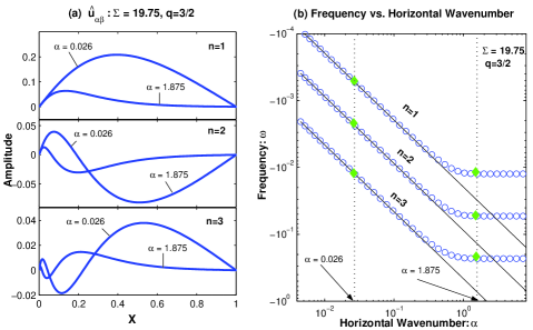
Figure 1: Results from normal mode theory in which $\Sigma=19.75$ and $q=3/2$ and $\Omega_{0}=1$. (a) The exact eigenfunctions for $\hat{u}_{\alpha\beta}$ depicted for the first three overtones each at two values of $\alpha$. The eigensolutions developed via the asymptotic theory lie exactly on the eigenfunctions for $\alpha=0.02$ where $A_{0}=1/2\delta$. (b) The frequencies $\omega$ as a function of $\alpha$ for the first three overtones are shown (open circles). The predicted frequencies using the asymptotic theory are shown with solid lines. The values corresponding to the eigenfunctions depicted in the left panel are designated with diamonds. Note that only the positive overtones (i.e., $n>0$) are shown here - the negative overtones are reflection symmetric about $x=1/2$ as discussed in the text.

4 Reflections and Speculation

1. A Speculation. With respect to the question of dynamics of wall-bounded rpCf, these results are quite suggestive. Rincon et al. (2007) showed that Rayleigh-stable anticyclonic rpCf appears not to show a transition into a turbulent state in the manner in which transition is observed in pCf flow (e.g., Waleffe, 2003). The strategy in those problems is to identify steady nonlinear solutions of the flow (usually by some continuation method from known solutions in otherwise unstable parameter regimes, e.g., Nagata, 1990, or forcing methods, Waleffe, 2003) and study their stability properties. If there are a collection of steady nonlinear structures, some of which unstable, then the transition into a turbulent state is thought to be approached. These states get easily triggered (bypass mechanism) because small scale disturbances in pCf get amplified due to the lift-up effect - a mechanism by which axisymmetric disturbances result in algebraic instability (Ellingsen & Palm, 1975). Rincon et al. (2007) however show that there are two problems with this approach when employed to identify structures of rpCf near the Rayleigh-stable line (e.g., near $q=2$ for Re $\rightarrow\infty$): that steady structures could not be identified and that the anti lift-up effect, which is the lift-up effect analog on the Rayleigh line, induces radial/vertical velocity fields that do not undergo the sorts of secondary instabilities that are characteristic of the induced azimuthal velocity fields generated by the lift-up effect in pCf flow.

Since the linear analysis of the inviscid Rayleigh-stable rpCf shows that for a given $\alpha$ and $\beta$ there are conditions where there exists a countable number of oscillating modes, we openly speculate here that one might consider identifying oscillating nonlinear structures instead of steady ones. Perhaps one strategy would be to (i) identify oscillating nonlinear states in the infinite Reynolds Number case (Re $=\infty$) and then (ii) ratchet down Re and follow/study the structures and their activity until either (iii) one identifies a Re of transition, if a unique one exists free of hysteretic effects or determine if, as Rincon et al. (2007) suggest, rpCf exhibits the character of a chaotic saddle. However we note that identifying oscillating (travelling wave) nonlinear solutions is difficult in plane Poiseuille flow (pPf) as Toh & Itano (2003) have recently shown. However, it might be easier to identify such structures in rpCf because of the presence there of linear oscillations whereas such oscillations are absent in linearized pPf.

2. Some Reflections. An individual wavemode subject to SBC, i.e. $\sim\exp{(ikX+i\alpha Y+i\beta Z)},$ where $k,\alpha$ and $\beta$ are wavenumbers as before, was shown by Balbus & Hawley (2007) to be an exact solution of the nonlinear equations of motion (i.e. 2-5). This is because this SBC waveform ansatz, together with the incompressibility condition, results in the nonlinear terms exactly cancelling to zero for each velocity component. Given (10-11) and (13) it follows that for these solutions the following holds,

$$\frac{d{\cal E}}{dt}=\frac{dE}{dt},$$

where $E$ is the disturbance kinetic energy of the wavemode (see 10). From (11) it follows that these disturbances conserve the shear energy $E_{{\rm shear}}$. A study of the form of $E_{{\rm shear}}$ shows that this is a natural outcome due to the symmetry of the modes with $\alpha,\beta\neq 0$. However, for modes in which $\alpha=\beta=0$, an inspection of the governing equations of motion in the SC shows that it necessarily follows that the corresponding azimuthal velocity mode, i.e. which is uniform in the vertical and azimuthal directions, is zero. Thus, by its very construction, these exact nonlinear modes as a result of SBC cannot support nonlinear modifications to the shear. Consequently, such alterations can occur only via three-wave interactions (Balbus & Hawley, 2007). We note that no such disturbances are supported in CBC flows - there always exists some amount of self-interaction for most modes of the system.

We note that for a general collection of perturbations utilizing SBC, (13) says that $\dot{\cal E}\neq 0$. The fluctuations in the total energy relate directly to the lateral exchange of kinetic energy from radially neighboring copies of the shearing box, where azimuthal velocities enter or exit boosted by the difference in the background shear velocities between the two boundaries - the quality of this exchange is a result of the type of correlations imposed upon the disturbances. For SBC it means that these correlations are set a priori by the periodic length scale of disturbances which is set to be on the scale of the box $L$ (e.g. see Regev & Umurhan, 2008). By contrast, the imposition of no-normal flow boundary conditions removes this source of energy into and out of the domain for problems invoking CBC, thus $\dot{\cal E}=0$ in that case.

We feel that these observations about the differences between CBC and SBC, together with recent results, raises more questions that need to be resolved. For instance, linear disturbances of the CBC type are understood not to result in decay because of reflections off of the channel walls. SBC conditions, on the other hand, support modes which can result in fluctuations of the total energy depending on the correlations that exist across the radial boundaries. It is interesting, therefore, that Lesur & Longaretti (2005) demonstrate the persistence of activity for simulations of the SSB (slightly below the Rayleigh line) using SBC while they report the presence of no such activity for CBC. On the other hand, there is in Shen et al. (2006) a recent demonstration of the decaying quality of disturbances in the SBC for flows run with $q=3/2$. Equally intriguing is that Lithwick (2007) shows that a single vortex may persist for a long time in a three-dimensional simulation of the SSB for $q=3/2$ using SBC which involves the complex interplay of three-wave mode interactions. It is interesting to us that while CBC conserves its total energy ${\cal E}$ no activity has yet been observed under Keplerian-like conditions while for SBC, which does not conserve its ${\cal E}$, sustained activity occurs in some cases while decay characterizes others.

Given the preceeding discussion it seems there are important questions to be asked:

1. What is the role of the non-self interacting wave modes resulting from the use of the SBC in the maintenance and/or destruction of activity in SSB simulations?

2. What influence does the prescribed velocity correlations, which result in the total energy not being conserved (cf. (13)) have on the overall evolution of general SSB simulations using SBC?

3. What influence does the non-self-interacting nature of these waves in the SBC have on the velocities on the radial boundaries of the system which, in turn, affects the amount of energy entering/leaving the system.?

4. How are we to understand these effects in relation to dynamics supported in the nonlinear response of flows utilizing CBC (i.e. wall-bounded rpCf)?

These observations and questions underscore the need for further analysis (also see Dubrulle, et al., 2005).

Acknowledgements. We thank the anonymous referee who gave us critical comments that helped us focus the presentation of this work and pointed us to earlier references. This work was partially supported by BSF grant number 0603414082.

References

- (1) Abramowitz, M. & Stegun, I. A., 1972, Handbook of Mathematical Functions, Dover, New York
- (2) Afshordi, N., Mukhopadhyay, B., & Narayan, R., 2005, ApJ, 629, 373
- (3) Balbus, S.A. & Hawley, J.F., 2006, ApJ, 652, 1020
- (4) Butler, K.M. & Farrell, B.F., 1992, Phys. Fluids A, 4, 1637
- (5) Case, K.M., 1960, Phys. of Fluids, 3, 143
- (6) Chagelishvili, G.D., Zahn, J.-P., Tevzadze, A. G., & Lominadze, J.G., 2003, A&A, 402, 401
- (7) Dubrulle B., Marie L. , Normand Ch., Richard D. , Hersant F.& Zahn J.-P. 2005, A&A, 429, 1
- (8) Ellingsen, T., and E. Palm, E., Phys. of Fluids, 18, 487
- (9) Goldreich, P. & Lynden-Bell, D., 1965, MNRAS, 130, 125
- (10) Ioannou, P.J. & Kakouris, A., 2001, ApJ, 550, 931
- (11) Jiménez, J., Kassinos, S.C. & Wray, A.A., 2006, Proceedings of the Summer Program 2006 (NASA Ames Research Center), 5
- (12) Johnson, B.M. & Gammie, C.F., 2005, ApJ, 626, 978
- (13) Knobloch, E. 1984, Geophys. Astrophys. Fluid Dyn., 29, 105
- (14) Korycansky, D.G., 1992, ApJ, 399, 176
- (15) Lesur, G. & Longaretti, P.-Y., 2005, 444, 25
- (16) Lithwick, Y. 2007 arXiv:0710.3868[astro:ph]
- (17) Longaretti, P-Y., 2002, ApJ, 587
- (18) Mukhopadhyay, B., Afshordi, N., & Narayan, R., 2005, ApJ, 629, 383
- (19) Nagata, M., 1986, JFM, 169, 229
- (20) Nusser, A., 2007, private communication.
- (21) Regev, O., and Umurhan O. M.,, In Press Astron. and Astrophys., arXiv:astro-ph/0711.0794 (2008).
- (22) Rincon, F., Ogilvie, G. I. & Cossu, C., 2007, A&A, 463 817
- (23) Rogallo, R., 1981, Numerical Experiments in Homogeneous Turbulence (Technical Memo 81315, Moffett Field, NASA/Ames)
- (24) Schmid, P. J. & Henningson, D.S., 2000, Stability and Transition in Shear Flows, Springer
- (25) Shen, Y, Stone, J.M. & Gardiner, T.A., 2006, ApJ, 653, 513
- (26) Sternberg, A., 2005, A search for Hydrodynamical Instabilities in Accretion Disks (Masters Research Thesis, Technion - Isreal Insitute of Technology).
- (27) Toh, S. & Itano, T., 2003, J. Fluid Mech., 481, 67
- (28) Umurhan, O.M. & Regev, O., 2004, A&A, 427, 855
- (29) Umurhan, O.M., 2006, MNRAS, 365, 85
- (30) Waleffe, F., 2003, Phys. Fluids, 15, 1517
- (31) Williams, P.T., 2000, Topics in Astrophysical Turbulence (Ph.D. Dissertation, University of Texas)
- (32) Williams, P.T., 2006, astro-ph/0607282
- (33) Yavneh, I., McWilliams J.C. & Molemaker, M.J. 2001, J. Fluid Mech., 448, 1
- (34) Yecko, P.A. 2004, A&A, 425, 385-393