Extraction of the photometric information : corrections

Abstract

We present here the set of corrections that will be applied to the raw data of the CoRoT mission. The aim is to correct the data for instrumental and environmental perturbations as well as to optimize the duty-cycle, in order to reach the expected performances of the mission. The main corrections are : the correction of the electromagnetic interferences, suppression of outliers, the background correction, the jitter correction and the correction of the integration time variations. We focus here on these corrections and emphasize their efficiency.

1 Introduction

There will be different levels of corrections performed on the scientific data.

The first level will be applied on the raw data and deals with first order correction associated with instrumental and environmental (e.g. background) perturbations. These will be based on calibrations performed on the ground before and during the launch as well as on-board. The goal of such first level corrections is to reach the expected performances in terms of noise and orbital components.

The first order corrections will be applied throught the so-called N0-N1 pipeline .

Corrections of higher levels will be performed in order to optimize the global performances of the mission, in particular in order to optimize the duty-cycle of the mission and to remove residual instrumental and environmental perturbations

The second order corrections will be applied throughout the so-called N1-N2 pipeline.

The first pipeline will be operated every one to seven days and therefore deals with short term corrections. The second pipeline will be operated once a run is finished.

These proceedings are organized as follows: In Sect. 2 we describe the content of N0-N1 pipeline and in Sect. 3 that of the N1-N2. The different corrections applied in the N0-N1 pipeline are detailed in Sections  2.1 to 2.7.

2 N0-N1 pipeline

The corrections applied to the star light-curves (LC hereafter) in the N0-N1 pipeline are the following:

• offset subtraction (see Sect. 2.1)

• suppression of the outliers (see Sect. 2.2)

• correction of the electromagnetic interferences (EMI, see Sect. 2.3)

• gain correction (to transform digitized data into electrons, see Sect. 2.4)

• integration time correction (see Sect. 2.5)

• background subtraction (see Sect. 2.6)

• jitter correction (see Sect. 2.7)

Before performing these treatments we need to carry out the offset and background measurements. For the offset measurements, the treatments are the following:

• correction of electromagnetic interference (see Sect. 2.3)

• suppression of the outliers (see Sect. 2.2)
  

  For the background measurements, we must apply in addition the following treatments:

• offset subtraction

• gain correction (see Sect. 2.4)

• calibration of the sky background aacross the field of view in order to remove a posteriori the background contribution to the star LCs (see Sect. 2.6).

Each of the above-mentioned treatments is detailed in Sects 2.1-2.7.

2.1 Offset

The offset of the electronic chain is measured on-board for each time step (1s for the astero channel and 32s for the exo-planet channel).

For the astero channel the offset is subtracted from the star and background LCs on-board. However the offset is subject to electromagnetic interferences (see Sect. 2.3) that will only be corrected afterwards on ground. Moreover, although these offset measurements are corrected on-board for outliers (e.g. cosmic impacts or glitches), the residual outliers will be removed on ground (see Sect. 2.2). We must then go back to the offset subtraction performed on-board and subtract instead the offset treated on ground.

For the exoplanet channel, the electronic offset is not subtracted from the star and background LCs on-board. The offset measurements are processed on ground to correct them for EMI and cosmic impacts (or glitches). Afterwards, they are subtracted from the LCs of the exoplanet channel.

2.2 Outliers

For the exo channel, the on-board measurements (background and stars) are not corrected for the outliers (e.g. cosmic impacts or glitches). This correction is applied on ground.

For the astero channel, although the measurements are corrected for outliers on-board, this correction may not be fully efficient - in particular when the satellite crosses the South Atlantic Anomaly. This is why the measurements from the astero channel are re-processed on ground in order to correct them for residual cosmic impacts (or glitches).

Several standard algorithms will be applied in order to correct the LC for outliers.

2.3 Electromagnetic interferences

2.3.1 Description and consequences

The charge transfer and readout performed on one CCD induces electromagnetic interferences (EMI hereafter) on all the three other CCDs (see Pinheiro da Silva et al, this volume).

On the exoplanet channel, during a 32s integration cycle, the first 23s are used to transfer and readout the charges. During the 9 remaining seconds, no more readouts are performed and the electronic chain does not interfere with the other CCDs anymore. On the astero channel, the charge transfer and readout are performed periodically each second and take less than 1s. As a consequence, the EMIs induced by the CCDs of the exoplanet chains on the CCDs of the astero channels occur during the first 23 exposures of a 32s cycle and cease during the 9 remaining exposures. The amplitudes and shapes of these EMIs depend on the position of the astero target being perturbed by the exoplanet CCDs. However these perturbations are strictly periodic (period of 32s). The patterns of the EMIs seen on the CCD of the seismo channel are shown in Fig. 1

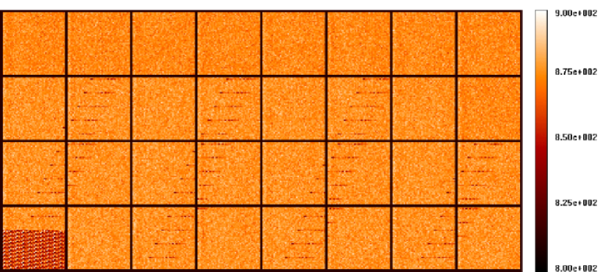
Figure 1: The pattern induced by the EMIs on the seismo CCD. Each box corresponds to an exposure of 1s; 32 exposures are represented.

In the same way the charge transfer and readout performed on the seismo CCD induce EMIs on the exo CCD. The patterns corresponding to those EMIs are shown in Fig. 2. Their shapes depend on the position of the astero targets.

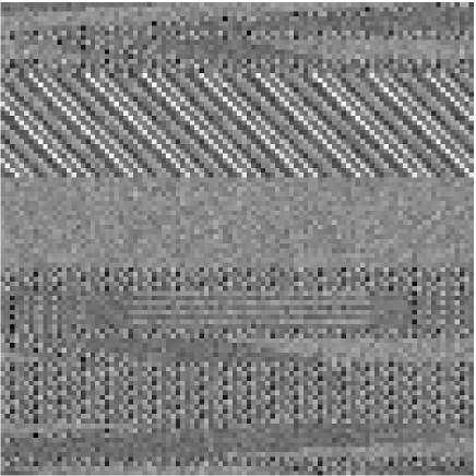
Figure 2: The pattern induced by the EMIs on the exo CCD.

2.3.2 Effects on the photometry

The perturbations induced by the EMIs on the offset measured on the astero channel are illustrated in Fig. 3. As seen in the Fig. the first 23 exposures of a 32s cycle have a larger offset level than the 9 remaining exposures. On the other hand, the EMI induced by the CCDs of the astero channels on the CCDs of the exoplanet channels occur each second and the associated perturbations are constant in time for the exposures of the exo channel.

Figure 3: Offset of the electronics as measured on the astero CCD.

Their amplitudes and shapes also depend on the positions of the astero targets on the astero CCDs.

For both channels the perturbations induced by the EMIs on the LCs (star, background) or the offset measurements are equivalent to a shift of the electronic offset with respect to the nominal level of the electronic offset. For the astero channel this shift varies with time and depends on the position of the target on the CCD. For the exoplanet channel however, this shift is constant with time but is inhomogeneous in space and hence differs from a target to another.

Such shifts of the electronic offset introduce biases on the absolute values of the measured target fluxes. However the absolute value of the target flux is not relevant for the main scientific goals of the mission. Nevertheless, if we are interested in the absolute values of the measured fluxes, such corrections are required. In addition, for the astero channel, as the perturbations induced by the EMIs change during a 32s cycle, their variations with time are undesirable as it decreases the efficiency of the outlier corrections.

2.3.3 Corrections

The shapes and positions of the EMIs on the CCD can be predicted precisely from the known electronic micro sequences that govern the charge transfers and readouts. However their amplitudes can only be characterized through calibrations.

Exo channel:

To correct the perturbations induced by the EMIs on exoplanet LCs we first calibrate the EMIs perturbations expected for each different electronic micro-sequences (see Pinheiro da Silva et al, this volume). ¿From this calibration and according to the way the windows of the astero CCDs are settled, we derive next the EMIs patterns as shown in Fig. 2. Then, for each target, we integrate the piece of the pattern that falls in the target template. This gives us a value of the shift induced by the EMIs on the LC for each target. Again, as the amplitude of the EMIs motif can change on a large scale, we can repeat the calibration and the correction processes periodically.

Astero channel:

For the Astero channel we can either perform a correction similar to the one applied for the exo-channel or perform an empirical correction.

In the first method, we begin by calibrating the EMIs perturbations expected for each different electronic micro-sequence. From this calibration we derive, for each window target, the expected perturbations for all phases of a 32s cycle (see Fig. 3). These perturbations depend on the way the windows of the astero CCDs are programmed. We next integrate the piece of the pattern that falls in the target mask. This gives us a value of the shift induced by the EMIs on the LC for each target

In the second method, we proceed as follows: As the perturbations are periodic with a period of 32s, we average the offset sequence at constant phase $\phi$, where the phase $\phi$ of the offset sequence is by definition $\phi\equiv$ t modulo 32 where $t$ is the time (in seconds, arbitrary origin). The result is shown in Fig. 4 for offset measurements. As seen in the Fig., the offset stands at a high level during 23 seconds and then remains at a lower level during the remaining 9 seconds of the 32s cycles. Once the motif of the EMI perturbation is calibrated in this way, we apply this motif on the offset sequence to correct it. However, as the amplitude of the motif can change on larger time scales, we split the offset sequence in an adequate number of sub-series. We then perform the calibration and the correction on each sub series.

Figure 4: Offset of the electronic (Fig. 3) averaged at constant phase $\phi$ (see text).

2.4 Gain

The gain of the electronic chain and of the CCD have been measured on ground during the calibration of the camera and the electronics. All the lightcurves of both channels will be multiplied by the gain in order to convert ADU into electrons.

During the mission, periodic calibrations of the gain (electronics +CCD) will be performed. However, the quality of those calibrations will not be high enough to derive the absolute value of the gain. However, they will allow us to characterize the variation of the gain during the life of the instrument and to apply afterwards a gain correction that will take into account its long term variation.

2.5 Integration time variations

The CCD charge transfer and readout is controlled by a clock inside the instrument (Quartz Instrument, QI hereafter). Thermal control is performed on the QI which prevents it from undesirable large fluctuations. Therefore variations in the QI with respect to the Universal Time (UT) are expected to be small (less than $\sim$ 1 ppm per second).

However, each 32s the charge transfer is synchronised with respect to the clock located inside the Proteus platform (Quartz Platform, QP hereafter). As a consequence the first 31 exposures are controlled by the QI while the (last) 32nd exposure is controlled by the QP.

This QP is not thermally controlled and hence is subject to significant variations with the temperature of the platform. The latter is expected to vary by a few kelvin during an orbit and the temperature coefficient of the QP is expected to be of the order of $\sim$ 2 ppm/K. Therefore variations of QP frequency of the order of few ppm are expected during an orbit.

Consequently, the integration time of the first 31 exposures is expected to remain almost constant while that of the 32nd exposure is expected to vary by $\sim 10^{-4}$ second if we assume a variation of the platform temperature of $\Delta T\simeq$ 2 K. This clock variation induces a flux variation at the orbital frequency of the order of $\sim 4$ ppm for an observation of 5 days. This is two times larger than the requirements.

Fortunately, each 32s the platform will provide, through the telemetry, the GPS (Global Positioning System) pulses received by the platform and the values of the QP counters when those pulses are received. ¿From this information, we will then be able to measure the variation of the QP with respect to the UT. In turn, this will allow us to correct the variation of the integration time of the 32nd exposures. This correction consists of multiplying the flux of the 32nd exposures by the ratio of the nominal integration time and the actual duration of the 32nd exposures (the latter being derived from the measured variations of the QP).

This correction efficiently removes the perturbations induced by the variations of the QP on the astero LCs. Furthermore it is so small that it doesn’t significantly change the (Poisson) statistics of the charge collected by the CCD.

For the exoplanet channel, the CCD charge transfer and readout are synchronised with respect to the QP. Therefore the flux measured on the exoplanet channel will also suffer from the variations of QP. The level of the flux perturbation induced by the QP variations will be of the same level as that expected for the astero channel. Thus it will be below the requirements imposed on the exoplanet channel. Nevertheless, this flux perturbation will be corrected in the same manner.

2.6 Background

The correction for sky background is a standard procedure in the reduction process of photometric data and basically consists of the subtraction of the sky background level from the photometric measurements of the star.

CoRoT Background Windows — To measure the sky background light, CoRoT has background windows distributed over each CCD, as shown in the Tab.1. The background windows on the CCDs of the SEISMO channel are larger, but binned. The modes oversampled (OV) and non-oversampled (NOV) of the EXO channel have background windows of the same size, but different in number per CCD.

Channel	CCD	Number of	Size	Binning	Sampling
		windows	(in pix)	(in pix)	(in sec)
SEISMO	A1	5	$50\times 50$	$5\times 5$	1
	A2	5	$50\times 50$	$5\times 5$	1
EXO (OV)	E1	10	$10\times 10$	–	32
	E2	10	$10\times 10$	–	32
EXO (NOV)	E1	40	$10\times 10$	–	512
	E2	40	$10\times 10$	–	512

Table 1: CoRoT background windows.

2.6.1 Background Components

The background is made up of different components. The major contributors are the diffuse galactic background, the zodiacal light, the straylight from the Earth and the South Atlantic Anomaly (SAA). Other minor contributors are the moonlight, the parasite light due to diffusion and reflection of the stars’ light inside the instrument.

While the diffuse galactic background and the zodiacal light are almost constant over time, the Earth straylight and the SAA are periodic components and require special attention.

Earth Straylight — The level of incident Earth straylight increases when the satellite passes over the illuminated face of the Earth and is at a minimum when it passes over the dark face, as illustrated in Fig.5. The height and shape of the bumps depend on the orientation of the satellite orbital plane in relation to the Sun-Earth axis and the worst case occurs when the two are aligned as shown in Fig.6.

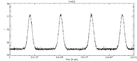
Figure 5: Earth straylight light curve. The bumps occur when the satellite passes over the illuminated face of the Earth.

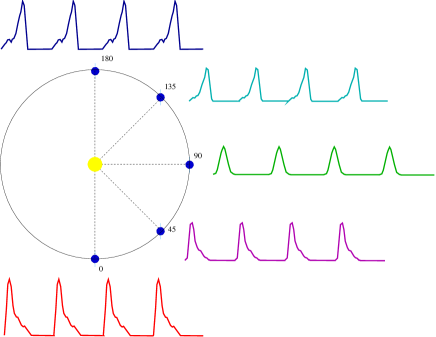
Figure 6: The curve of the Earth straylight changes as a function of the orbital position of the Earth around the Sun.

2.6.2 Effects on the photometry

The Earth straylight introduces a periodic signal with period equal to orbital period (1h 43min) in the measured light curve of the stars. As shown in Fig.7 in the Fourier spectrum, it appears as a peak with the fundamental frequency of $162\mu Hz$ and a series of harmonic frequencies, with low amplitude, but that can trouble the detection and analysis of pulsation frequencies of the observed pulsating stars.

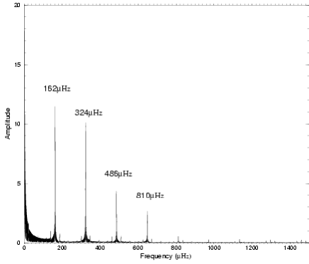
Figure 7: Discrete Fourier transform of the Earth straylight curve. The fundamental frequency is $162\,\mu Hz$.

Earth straylight can also affect the detection of planetary transits in the EXO channel. If a planetary transit occurs while the satellite is passing over the illuminated face of the Earth, the increase in the background light level can compensate for the small variations in the light curve of the star.

2.6.3 Sky Background Gradient

Due to the asymmetry of the CoRoT optical system, the diffusion of the sky background light over the focal plane is non-homogeneous. We don’t know exactly if the non-homogeneity is regular or irregular and how strong the gradient is. However, theoretical studies suggest a regular gradient as shown in Fig.8.

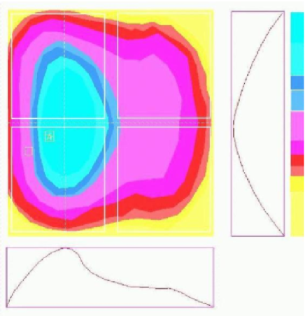
Figure 8: Theoretical diffusion of the sky background light over the focal plane.

2.6.4 Correction

The simplest procedure for correction by sky background of a star light curve is to subtract from each measurement of the star light the sky level measured from the nearest background window. This procedure assumes that the background is homogeneous, at least, in the neighborhood of the two windows. However, in presence of a non-negligible gradient, the sky levels for the two windows can be significantly different and this procedure will not completely subtract the sky from the star light curve.

In order to avoid this problem, we need take into account the sky background gradient. For this, the gradient is modeled by a spatial function $f(x,\,y)$ over the whole CoRoT focal plane, from the combined sky measurements of all CCDs. Different trial functions are fitted and the one that provides the best fit is chosen as model for the background gradient.

In the fitting, it is necessary to take into account that the gains of the channels are different. For this reason we introduce the gain parameters, $g_{ij}$, where the index $i$ refers to the CCD (A1, A2, E1, E2) and the index $j$ refers to the CCD’s channel (left or right). In fact, the correction by gain is done in a previous step of the data treatment, using values experimentally determined. This way, the determination of the parameters $g_{ij}$ is used to refine the gain correction.

The trial functions used are listed in Tab.2. Functions of higher order can be tried, if needed. Fig.9 shows the result of a fitting of a Gaussian model for the background gradient from simulated data.

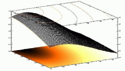
Figure 9: Fitting of a Gaussian model for $f(x,\,y)$ from simulated data.

As a result, a time series is obtained for each one of the parameters of the model function which allow us to calculate, by interpolation with respect to time, the correct sky level over each star window and for any moment in time (see Fig.10).

Gradient		Number of
Type	Function	Parameters
Constant	$f(x,\,y)=g_{ij}\,a_{0}$	9
Linear	$f(x,\,y)=g_{ij}\,(a_{0}+a_{1}\,x+a_{2}\,y)$	11
Quadratic	$f(x,\,y)=g_{ij}\,(a_{0}+a_{1}\,x+a_{2}\,y$
	$+a_{3}\,xy+a_{4}\,x^{2}+a_{5}\,y^{2})$	14
Gaussian	$f(x,\,y)=g_{ij}\,\left[a_{0}\,\exp\left(a_{1}(x-a_{2})^{2}\right.\right.$	13
	$\left.\left.+a_{3}(y-a_{4})^{2}\right)\right]$

Table 2: Trial functions for modeling of the sky background gradient.

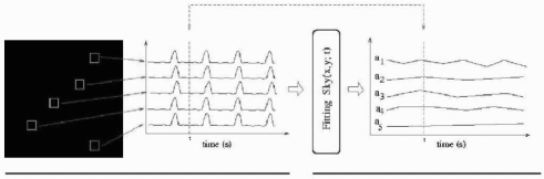
Figure 10: From the measurements of the sky background obtained in the instant $t$ a spatial function $Sky(x,\,y)$ is fitted and its parameters are calculated. By doing this for each time step, a parameters time series is obtained.

The modeling of the sky background as described above assumes that the gradient is non-homogeneous, but relatively regular. This hypothesis can be tested a posteriori from the comparison of the variance for the fitting $\rm{Var}_{\rm{mod}}$ with the average variance of the background measurements, $\rm{Var}_{\rm{bg}}$:

comparison	gradient	procedure to be used
$\rm{Var}_{\rm{mod}}<\rm{Var}_{\rm{bg}}$	non-homogeneous,	model $f(x,\,y;\,t)$
	but regular
$\rm{Var}_{\rm{mod}}\simeq\rm{Var}_{\rm{bg}}$	homogeneous	$f(x,\,y;\,t)=\rm{constant}$
		or the nearest sky window
$\rm{Var}_{\rm{mod}}>\rm{Var}_{\rm{bg}}$	non-homogeneous	local triangularization
	and irregular

For non-homogeneous and irregular gradients, the calculation of the sky level over the star window by local triangularization is used. This procedure calculates the parametric equation of the plane defined by the measurements of the three nearest background windows and then calculates the background level for the star window position. This technique is illustrated in Fig.11.

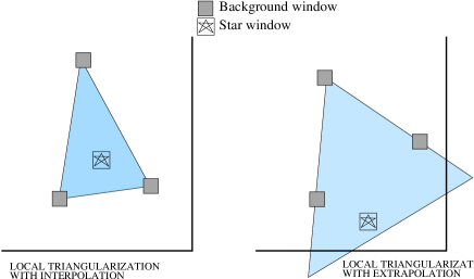
Figure 11: The technique of local triangularization used to calculate the background level over a sky window from the measurements of the three nearest sky windows.

2.7 Jitter

The idea here is to correct the LCs for the edge effects and/or chromatic contamination provoked by satellite jitter in the fixed photometric aperture in both channels. The importance of this correction is not only seen in the improvement of the S/N ratio of the photometric curves, but also in better definition of seismo photometric masks, because the quality we can achieve in jitter correction is also taken into consideration when calculating the optimal mask. See item VI.3. As the seismo and exo channels have different goals, their designs are not the same, which means that different approaches can be used to conceive the corrections. Below the proposed methods to correct each channel are described.

2.7.1 Seismo channel

For the seismo channel the CoRoT instrument was specified in a way that the jitter photometric noise is negligible for stars of magnitude 6.  However the correction of this source of noise must be carried out for less bright stars, or if the AOCS degrades.

Fig. 12 illustrates the problem in frequency. The component of frequency indicated by the arrow is due to jitter and must be corrected.

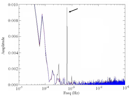
Figure 12: Fourier spectrum of non corrected (black) and corrected (blue) LCs

Two methods of correction have been developed for this channel with a single idea behind them: to estimate the best correction according to the equation:

$$F_{c}=K(\Delta x_{i},\Delta y_{i})F_{m},$$ (1)

where $Fc$ is the corrected flux, $K(\Delta x_{i},\Delta y_{i})$ is the so called correction surface, $Fm$ is the measured flux and $\Delta x_{i},\Delta y_{i}$ are the displacement of the target with respect to its average position. This means that once created, the correction surface in Fig. 13, can be used to apply the adequate factor of correction to each measured point of the photometry as a function of the pointing error at that instant.

Below we describe the two ways this surface can be created.

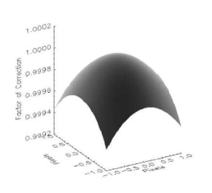
Figure 13: Example of correction surface for jitter correction in seismo field

PSF Model:

This is a model-based method that consists of creating a surface based on the evaluation of loss of flux from the Point Spread Function (PSF) model and the photometric aperture. The PSF is gotten at the beginning of life of the satellite (see Pinheiro da Silva et al, this volume).

Signal correlation:

By examining the correlation among calculated displacement (x and y jitter) and output (measured flux), we estimate the average loss of flux for a pre-defined jitter variation grid. We average over a period of more than 10 orbits to build the correction surface from the COROT signal itself. This needs no accurate knowledge of the PSF. For a more detailed description of the various methodologies see [Drummond, R. et al. (2006)].

2.7.2 Exo channel

The seismo channel is almost insensitive to the variation of jitter, but the exo channel is highly sensitive to the pointing variation of the satellite. This is true not only because of the lower number of pixels in the mask, but also because of the use of chromatic photometry that induces chromatic contaminations. As an example, the Fig. 14 shows two time series curves before and after correction, where we can see a significant gain in the SNR.

Again, as in the seismo channel, we are interested in estimating the correction factor $K(\Delta x_{i},\Delta y_{i})$. Two methods are considered here and they are explained below.

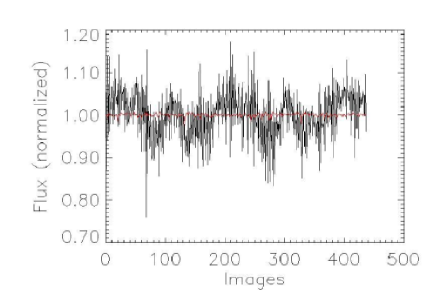
Figure 14: Exo LCs before (black) and after (red) jitter correction

PSF Model:

This is a simple extension of the method applied to the seismo channel. Instead of creating just one correction surface, four surfaces are calculated, one for each color. The difference in each is the mask it uses. Fig. 15 illustrates the surfaces for each color.

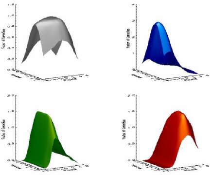
Figure 15: Correction surfaces for mono and chromatic jitter correction in exo field

Integrated spectrum:

This method is based on the integrated spectrum of the star (Fig. 16 that is simply the summation of all pixels in one direction (columns in this case). Here it is not necessary to have an accurate knowledge of the PSF. A few images are enough to compute the integrated spectrum. As the chromatic effects are the most significant in exo photometric apertures, only this phenomenon is evaluated. This means that here we are just interested in 1-D correction and ithis is done by the means of the estimation of the flux loss in the chromatic borders of the integrated spectrum. Chromatic borders are calculated using energy thresholds. Thus, it is possible to recover the photometric signal lost as a function of jitter. This method demands a larger mask to guarantee that edge effects will be negligible.

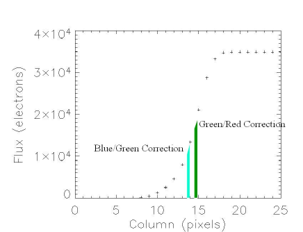
Figure 16: Star integrated spectrum for chromatic jitter correction in exo field

3 N1-N2 pipeline

The corrections performed by the N1-N2 pipeline have not yet been completely specified, since we will need the real data to do this.

They are different for the exo and astero channels. We describe below the current content of this pipeline, successively for the astero channel (Sect. 3.1) and the exo channel (Sect. 3.2).

3.1 Astero channel

We will first process the so-called “imagettes”. These are small images of a star that will be downloaded every 32s for some of the targets. A Point Spread Function (PSF) fitting will be applied to those “imagettes” in order to:

• extract the photometry of the star

• detect cosmic impacts

• derive the sky background

For bright stars ($m_{v}\sim 6$), the photometry based on PSF fitting is shown to be less accurate than the aperture photometry performed on-board. The former is only useful for fainter stars ($m_{v}\sim 8$) or when the satellite crosses the SAA.

On the star LCs, we will first transform the Universal Time (UT) into the barycentric time (BT hereafter) in order to move to a time reference that has a constant Doppler shift with respect to the time reference relative to the star.

Furthermore, in the on-board reference time (UT), the sampling is almost constant while in the barycentric time reference, this is no longer the case. This is a problem if one performs a Fast Fourier Transform (FFT) because the FFT assumes that the measurements are evenly sampled. In order to perform a FFT, we interpolate the LC with respect to an evenly sampled BT grid.

Finally, we integrate the LC over 32s.

When crossing the SAA, the photometry extracted from the “imagettes” on the basis of a PSF fitting will be more accurate. Hence, during the SAA crossing, we will patch the LC with the photometry of the “imagettes”. This procedure will increase the duty-cycle.

If the sky background derived from the “imagettes” turns out to be less biased than the one subtracted by the N0-N1 pipeline (see Sect. 2.3), we will cancel the sky background correction performed by the the N0-N1 pipeline and subtract instead the one derived from the “imagettes”.

Finally, the correction of the long term variation of the gain will be performed on the complete LC (see Sect. 2.4).

3.2 Exo channel

The exo channel N1-N2 pipeline will be divided in two parts.

The first part will be devoted to additional instrumental corrections which are not fully taken into account in the N0-N1 pipeline. Two corrections are foreseen at the moment: (i) a correction for residual cosmic events near the SAA, and (ii) a correction for residual background signal. The correction for cosmic impacts envisaged in the N0-N1 pipeline (see Sect. 2.2) is indeed expected to leave residuals when the satellite is at the edge of the SAA, before exo treatments stop. The aim of the background correction in the N1-N2 pipeline is to complement the N0-N1 background correction of Sect. 2.6 in case the background signal is inhomogeneous across the field-of-view. The algorithms to be applied still need to be defined. Additional residual corrections may be implemented during the mission if new instrumental effects are identified.

The second part will be devoted to a rough characterization of the level of stellar variability, in the form of a numerical parameter which will be included in the header of the data. The aim of this parameter will be to help to select the best candidates where low level transit events can be searched for. A method based on a Fourier analysis of the lightcurve will be implemented at the beginning of the mission. This method will be refined later on and/or complemented by new indicators of stellar variability.

The content of this paper represents the work of all the CoRoT ground segment team in Meudon (LESIA) and in Orsay (IAS).

References

- [Drummond, R. et al. (2006)] Drummond, R., De Oliveira Fialho, F., Vandenbussche, B., Aerts, C. & Auvergne, M.., 2006, PASP, 118, 844