Models of diffusion of Galactic Cosmic Rays from Super-bubbles

Abstract

Super-bubbles are shells in the interstellar medium produced by the simultaneous explosions of many supernova remnants. The solutions of the mathematical diffusion and of the Fourier expansion in 1D, 2D and 3D were deduced in order to describe the diffusion of nucleons from such structures. The mean number of visits in the the case of the Levy flights in 1D was computed with a Monte Carlo simulation. The diffusion of cosmic rays has its physical explanation in the relativistic Larmor gyro-radius which is energy dependent. The mathematical solution of the diffusion equation in 1D with variable diffusion coefficient was computed. Variable diffusion coefficient means magnetic field variable with the altitude from the Galactic plane. The analytical solutions allow us to calibrate the code that describes the Monte Carlo diffusion. The maximum energy that can be extracted from the super-bubbles is deduced. The concentration of cosmic rays is a function of the distance from the nearest super-bubble and the selected energy. The interaction of the cosmic rays on the target material allows us to trace the theoretical map of the diffuse Galactic continuum gamma-rays. The streaming of the cosmic rays from the Gould Belts that contains the sun at it’s internal was described by a Monte Carlo simulation. Ten new formulas are derived.

PACS numbers: 96.40.-z , 96.50.Pw , 05.40.Fb

1 Introduction

The spatial diffusion of cosmic rays (CR) plays a relevant role in astrophysics due to the fact that the binary collisions between CR and interstellar medium are negligible, e.g. [1, 2]. In these last years a general consensus has been reached on the fact that particle acceleration in Supernova Remnants , in the following SNR, may provide CR at energies up to $10^{15}eV$ [3] and probability density function in energy p(E)$\propto E^{-2}$. Some of methods for the numerical computation of the propagation of primary and secondary nucleons have been implemented [4, 5] . The previous efforts have covered the diffusion of CR from SNR [6, 7, 8] but the SNR are often concentrated in super-bubbles (SB) that may reach up to 800 pc in altitude from the Galactic plane. The complex 3D structure of the SB represents the spatial coordinates where the CR are injected. We remember that the super-bubbles are the likely source of at least a substantial fraction of GCRs; this can be shown from the analysis of the data from the Cosmic Ray Isotope Spectrometer (CRIS) aboard the Advanced Composition Explorer (ACE) and in particular the 22Ne/20Ne ratio at the cosmic-ray source using the measured 21Ne, 19F, and 17O abundances as ‘tracers” of secondary production [9]. Further on is known that $\approx~{}75\%$ of supernova occur in super-bubbles, and $\approx~{}88\%$ of the cosmic-ray heavy particles are accelerated there because of the factor of  3 enhanced super-bubble core metallicity [10, 11] .

In order to describe the propagation of CR from SB, in Section 2 we have developed the mathematical and Fourier solutions of the diffusion in presence of the stationary state and the Monte Carlo simulations which allow us to solve the equation of the diffusion from a numerical point of view . The case of random walk with variable length of the step was analysed in Section 2.5. The physical nature of the diffusion as well as evaluations on transit times and spectral index are discussed in Section 3. The 3D diffusion with a fixed length of a step and injection points randomly chosen on the surface of the expanding SB was treated in Section 4.

2 Preliminaries

In this section the basic equations of transport are summarised, the rules that govern the Monte Carlo diffusion are set up and the various solutions of the mathematical and Fourier diffusion are introduced. The statistics of the visits to the sites in the theory of Levy flights and it’s connection with the regular random walk are analysed. It is important to point out that the mathematical and Monte Carlo diffusion here considered cover the stationary situation.

2.1 Particle transport equations

The diffusion-loss equation as deduced by [12] ( equation (20.1) ) for light nuclei once the spallation phenomena are neglected has the form

$$\frac{\partial N_{i}}{\partial t}=D\nabla^{2}N_{i}+\frac{\partial}{\partial E}[b(E)N_{i}]+Q_{i},$$ (1)

here $N_{i}$ is the number density of nuclei of species i , $\nabla^{2}$ is the Laplacian operator , D is the scalar diffusion coefficient, $\frac{\partial}{\partial E}[b(E)N_{i}]$ takes account of the energy balance, and $Q_{i}$ represents the injection rate per unit volume.

When only protons are considered and the energy dependence is neglected Equation (1) becomes

$$\frac{\partial P(x,y,z,t)}{\partial t}=D\nabla^{2}P(x,y,z,t)\quad,$$ (2)

where P is the probability density , see [13] (equation 12.34b ). In this formulation the dependence for the mean square displacement $\overline{R^{2}(t)}$ is, see [13] (equation. 8.38 ),:

$$\overline{R^{2}(t)}=2dDt\quad(t\rightarrow\infty)\quad,$$ (3)

where d is the spatial dimension considered. From equation (3), the diffusion coefficient is derived in the continuum :

$$D=(t\rightarrow\infty)\frac{\overline{R}^{2}}{2dt}\quad.$$ (4)

In the presence of discrete time steps on a 3D lattice the average square radius after N steps, see [13] (equation 12.5 ), is

$$\langle R^{2}(N)\rangle\sim 2dDN\quad,$$ (5)

from which the diffusion coefficient is derived

$$D=\frac{\langle R^{2}(N)\rangle}{2dN}\quad.$$ (6)

If ${\langle R^{2}(N)\rangle}~{}\sim~{}N$ , as in our lattice :

$$D=\frac{1}{2d}\quad,$$ (7)

when the physical units are 1 and

$$D=\frac{1}{2d}\lambda v_{tr}\quad,$$ (8)

when the step length of the walker is $\lambda$ and the transport velocity $v_{tr}$.

Another useful law is Fick’ s second equation in three dimensions [14],

$$\frac{\partial C}{\partial t}=D\nabla^{2}C\quad,$$ (9)

where the concentration C(x,y,z) is the number of particles per unit volume at the point (x,y,z). We now summarise how Fick’ s second equation transforms itself when the steady state is considered in the light of the three fundamental symmetries. In the presence of spherical symmetry, equation (9) becomes

$$\frac{1}{r^{2}}\frac{d}{dr}(r^{2}\frac{dC}{dr})=0\quad,$$ (10)

the circular symmetry (starting from the hollow cylinder) gives

$$\frac{d}{dr}(r\frac{dC}{dr})=0\quad,$$ (11)

and the point symmetry (diffusion from a plane) produces

$$\frac{d^{2}C}{dr^{2}}=0\quad,$$ (12)

in the case of constant D and

$$\frac{d}{dr}(D\frac{dC}{dr})=0\quad,$$ (13)

when D is a function of the distance or the concentration.

2.2 Monte Carlo diffusion

The adopted rules of the d-dimensional (with d=1,2,3) random walk on a lattice characterised by $NDIM^{d}$ elements occupying a physical volume $side^{d}$ (in the hypothesis of a stationary state and fixed length step) are specified as follows:

1. The motion starts at the center of the lattice ,

2. The particle reaches one of the $2\times d$ surroundings and the procedure repeats itself ,

3. The motion terminates when one of the $2\times d$ boundaries is reached ,

4. The number of visits is recorded on ${\mathcal{M}}^{d}$ , a d–dimensional memory or concentration grid ,

5. This procedure is repeated NTRIALS times starting from (1) with a different pattern ,

6. For the sake of normalisation the d–dimensional memory or concentration grid ${\mathcal{M}}^{d}$ is divided by NTRIALS .

2.3 Mathematical diffusion

The solutions of the mathematical diffusion are now derived in 3D,2D,1D and 1D with variable diffusion coefficient.

2.3.1 3D analytical solution

Consider a spherical shell source of radius b between a spherical absorber of radius a and a spherical absorber of radius c, see Figure 1 that is adapted from Figure 3.1 of [14] .

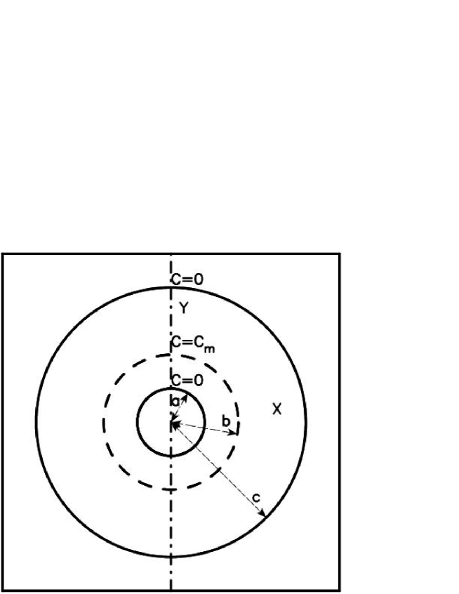
Figure 1: The spherical source is represented by a dashed line, the two absorbing boundaries with a full line.

The concentration rises from 0 at r=a to a maximum value $C_{m}$ at r=b and then falls again to 0 at r=c . The solution of equation (10) is

$$C(r)=A+\frac{B}{r}\quad,$$ (14)

where A and B are determined from the boundary conditions ,

$$C(r)=C_{{m}}\left(1-{\frac{a}{r}}\right)\left(1-{\frac{a}{b}}\right)^{-1}\quad a\leq r\leq b\quad,$$ (15)

and

$$C(r)=C_{{m}}\left({\frac{c}{r}}-1\right)\left({\frac{c}{b}}-1\right)^{-1}\quad b\leq r\leq c\quad.$$ (16)

These solutions can be found in  [14] or in [15] . The second solution (equation (16)) can be applied to explain the 3D diffusion from a central point once the following connection between continuum and discrete random walk is made

$$b = \frac{side}{NDIM-1}$$ (17)

$$c = \frac{side}{NDIM-1}(\frac{NDIM+1}{2}-1)\quad.$$

For example when $NDIM~{}\gg~{}1$ or $\frac{c}{b}~{}\gg~{}1$

$$C(r)\sim C_{{m}}\frac{b}{r}\quad,$$ (18)

in other words, the concentration scales as an hyperbola with unity represented by the mean free path b. The 3D theoretical solution as well as the Monte Carlo simulation are reported in Figure 2.

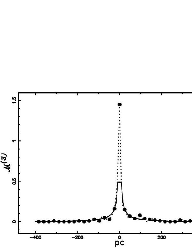
Figure 2: Values of ${\mathcal{M}}^{(3)}$ or concentration computed with equation (16) (full line) compared with the results of a Monte Carlo simulation (filled circles). The parameters are: NDIM=101, NTRIALS=100 and side=800pc.

2.3.2 2D analytical solution

The 2D solution is the same as the hollow cylinder. The general solution to equation (11) is

$$C(r)=A+Bln(r)\quad.$$ (19)

The boundary conditions give

$$C(r)=C_{{m}}\frac{ln(r/a)}{ln(b/a)}\quad a\leq r\leq b\quad,$$ (20)

and

$$C(r)=C_{{m}}\frac{ln(r/c)}{ln(b/c)}\quad b\leq r\leq c\quad.$$ (21)

The new 2D theoretical solution as well as the Monte Carlo simulation are reported in Figure 3.

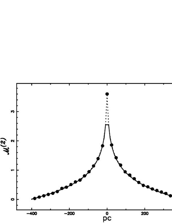
Figure 3: Values of ${\mathcal{M}}^{(2)}$ or concentration computed with equation (21) (full line) compared with the results of a Monte Carlo simulation (filled circles). The parameters are: NDIM=101, NTRIALS=4000 and side=800pc.

2.3.3 1D analytical solution

The 1D solution is the same as the diffusion through a plane sheet. The general solution to equation (12) is

$$C(r)=A+Br\quad.$$ (22)

The boundary conditions give

$$C(r)=C_{{m}}\frac{r-a}{b-a}\quad a\leq r\leq b\quad,$$ (23)

and

$$C(r)=C_{{m}}\frac{r-c}{b-c}\quad b\leq r\leq c\quad.$$ (24)

The 1D theoretical solution as well as the Monte Carlo simulation are reported in Figure 4.

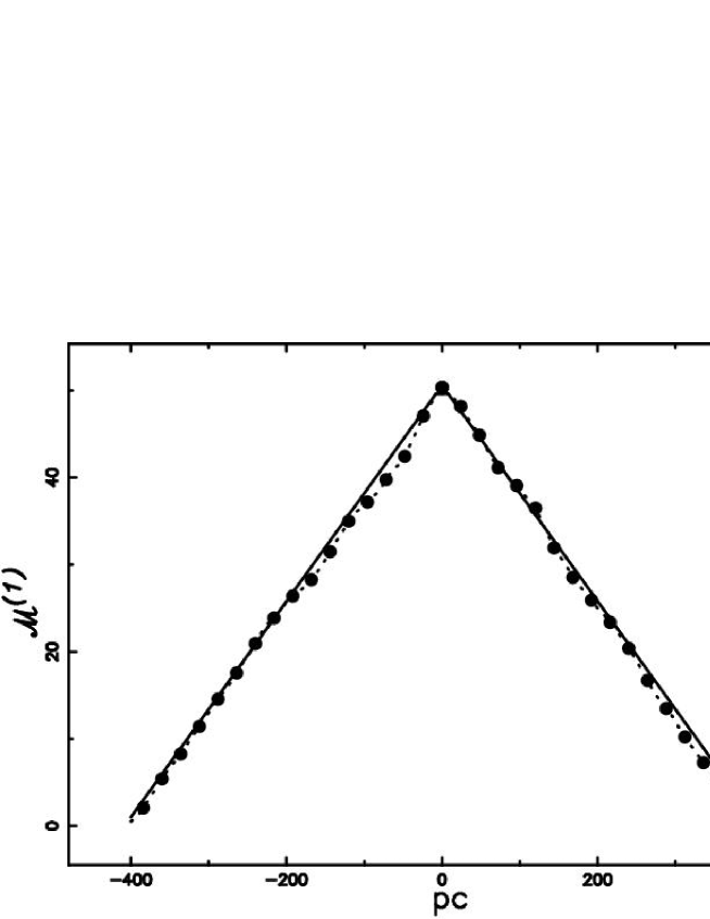
Figure 4: Values of ${\mathcal{M}}^{(1)}$ or concentration computed with equation (24) (full line) compared with the results of a Monte Carlo simulation (filled circles). The parameters are: NDIM=101, NTRIALS=100 and side=800pc.

2.3.4 1D analytical solution with variable D

The diffusion coefficient D is assumed to be a function ,f ,of the distance

$$D=D_{0}(1+f(r))\quad,$$ (25)

where $D_{0}$ is the value of D at the plane where the diffusion starts. On introducing the integral I defined as :

$$I=\int\frac{dr}{1+f(r)}\quad,$$ (26)

the solution to equation (13) is found to be ,

$$\frac{C-C_{1}}{C_{1}-C_{2}}=\frac{I_{1}-I}{I_{1}-I2}\quad,$$ (27)

where $C_{1}$ ,$C_{2}$ , $I_{1}$ and $I_{2}$ are the concentration and the integral respectively computed at $r=r_{1}$ and $r=r_{2}$ [15, 16]. For the sake of simplicity the diffusion coefficient is assumed to be

$$D=D_{0}(1+a_{D}(r-r_{1}))\quad,$$ (28)

where $a_{D}$ is a coefficient that will be fixed in Section 3.2.2 . A practical way to determine $a_{D}$ is connected with the interval of existence of r , $[r_{1},r_{2}]$, and with the value that D takes at the boundary

$$a_{D}=\frac{D(r_{2})/D_{0}-1}{r_{2}-r_{1}}\quad.$$ (29)

Along a line perpendicular to the plane the concentration rises from 0 at r=a to a maximum value $C_{m}$ at r=b and then falls again to 0 at r=c . The variable diffusion coefficient is

$$D=D_{0}(1+a_{D}(b-r))$$ (30)

$$when\quad a\leq r\leq b\quad,$$

and

$$D=D_{0}(1+a_{D}(r-b))$$ (31)

$$when\quad b\leq r\leq c\quad.$$

The solution is found to be

$$C(r)={\frac{\left(\ln\left(-{\it a_{D}}\,a+1+{\it a_{D}}\,b\right)-\ln\left(-{\it a_{D}}\,r+1+{\it a_{D}}\,b\right)\right){\it C_{m}}}{\ln\left(-{\it a_{D}}\,a+1+{\it a_{D}}\,b\right)}}$$ (32)

$$when\quad a\leq r\leq b\quad,$$

and

$$C(r)=-{\frac{{\it C_{m}}\,\left(-\ln\left({\it a_{D}}\,c+1-{\it a_{D}}\,b\right)+\ln\left({\it a_{D}}\,r+1-{\it a_{D}}\,b\right)\right)}{\ln\left({\it a_{D}}\,c+1-{\it a_{D}}\,b\right)}}$$ (33)

$$when\quad b\leq r\leq c\quad.$$

The new 1D theoretical solution when the diffusion coefficient is variable is reported in Figure 5.

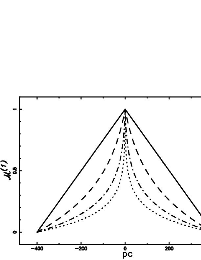
Figure 5: Values of ${\mathcal{M}}^{(1)}$ or concentration computed with equations (32) and (33) when a =-400 pc, b=0 pc and c=400 pc : $D(c)/D(b)=1.0001$ ( full line ), $D(c)/D(b)=10$ ( dashed ), $D(c)/D(b)=100$ ( dot-dash-dot-dash ), $D(c)/D(b)=1000$ ( dotted ).

Confront our Figure 5 with Figure 8 in [7] , where the density of primary CR is a function of the distance from the Galactic plane and different physical parameters.

2.4 Fourier Series

In the case of restricted random walk the most straightforward way to compute the mean number of visits is via the solution of the Fokker-Planck equation, which in the case of simple, symmetric random walk equation reduces to the diffusion equation [17]. Given the dimension d, the random walk takes place on a finite domain $D=[-L/2,L/2]^{d}\subset R^{d}$, and the boundaries are supposed to be absorbing. In this case the solutions of the diffusion equation can be obtained with the usual methods of eigenfunction expansion [17, 18] and they are cosine series whose coefficients decay exponentially, see equation (25) in [19]. The solutions particularized as a cuts along one axis are

$${\mathcal{M}}^{(1)}(x)=\frac{2}{L}\sum_{m=0}^{\infty}\kappa_{m}\cos\left[\frac{(2m+1)\pi x}{L}\right],$$ (34)

$${\mathcal{M}}^{(2)}(x,0)=\left(\frac{2}{L}\right)^{2}\sum_{m,l=0}^{\infty}\kappa_{ml}\cos\left[\frac{(2m+1)\pi x}{L}\right]\quad,$$ (35)

$${\mathcal{M}}^{(3)}(x,0,0)=\left(\frac{2}{L}\right)^{3}\sum_{m,l,j=0}^{\infty}\kappa_{mlj}\cos\left[\frac{(2m+1)\pi x}{L}\right],$$ (36)

with

$$a=\frac{L}{2}\quad,$$

$$\kappa_{m}=\frac{\left(2L^{2}\right)}{(2m+1)^{2}\pi^{2}}\quad,$$

$$\kappa_{ml}=\frac{\left(2L^{2}\right)}{\left((m+1)^{2}+(l+1)^{2}\right)\pi^{2}}\quad,$$

$$\kappa_{mlj}=\frac{\left(2L^{2}\right)}{\left((m+1)^{2}+(l+1)^{2}+(j+1)^{2}\right)\pi^{2}}\quad.$$

These three new solutions are the Fourier counterpart of the solutions of the mathematical diffusion (24), (21) and (16) respectively. The comparison between solution in 3D with methods of eigenfunction expansion, mathematical diffusion and Monte Carlo simulation is carried out in Figure 6.

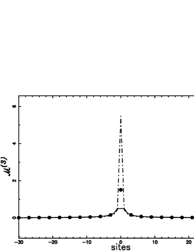
Figure 6: Profile of ${\mathcal{M}}^{(3)}$ versus the number of sites as given by Monte Carlo simulation with regular lengths step (filled circles ) + solution of the mathematical diffusion (full line ) + Fourier expansion (dot-dash-dot-dash line ) . The parameters are NDIM=101 , L=25, NTRIALS=10 000 , $m$, $l$ , $j$ ranging from $1$ to $21$.

2.5 Levy random walks in 1D

In the case of the Levy [20] random walk in 1D it should noted that $\delta x$, i.e. the single step, can be written as

$$\delta x=\xi l,$$ (37)

where $l>0$ is the length of the flight and $\xi$ is a stochastic variable taking values $1$ and $-1$ with equal probability. For the distribution of $l$ chose

$$p(l)=Cl^{-(\alpha+1)}\quad,$$ (38)

where $0<\alpha<\infty$, and then

$$p(\delta x)=1/2p(l)\quad.$$ (39)

Let ${\mathcal{S}}^{\alpha}$ denote the average number of visits to a site obtained via a Monte Carlo simulation ; when ${\mathcal{M}}^{\alpha}$ denotes the corresponding values given by the equation [21],

$${\mathcal{M}}^{\alpha}(x)=\frac{2}{L}\sum_{n=1}^{\infty}\frac{L^{\alpha}}{(n\pi)^{\alpha}D_{\alpha}}\sin\left(\frac{m\pi(x+a)}{L}\right)\sin\left(\frac{m\pi a}{L}\right)\quad,$$ (40)

where

$$D_{\alpha}=\frac{4}{\pi T}\left(\frac{L}{\pi}\right)^{\alpha}\sum_{m=1}^{\infty}\frac{(-1)^{m}}{(2m+1)^{1+\alpha}}\quad,$$ (41)

being

$$T=\sum_{x=0}^{L}{\mathcal{S}}^{\alpha}(x)\quad.$$ (42)

Once we calculate the constant in pdf (38) (probability density function) the Pareto distribution, P, is obtained [22]:

$$P(l;a,c)=\frac{ca^{c}}{l^{c+1}}\quad,$$ (43)

where $a\leq l<\infty$ , $a~{}>0$ , $c~{}>0$. The average value is

$$\overline{l}=\frac{ca}{c-1}\quad,$$ (44)

which is defined for $c>1$, and the variance is

$$\sigma^{2}={\frac{{a}^{2}c}{\left(-2+c\right)\left(-1+c\right)^{2}}}\quad,$$ (45)

which is defined for $c>2$. In our case the steps are comprised between 1 and $l_{max}$ and the following pdf , named Pareto truncated $P_{T}$ , has been used

$$P_{T}(l;l_{max},\alpha)=\Bigr{(}\frac{\alpha}{1-\frac{1}{l_{max}}}\Bigl{)}\frac{1}{l^{\alpha+1}}\quad.$$ (46)

The average value of $P_{T}$ is

$$\overline{l}=-{\frac{\alpha\,\left(-{{\it l_{max}}}^{\alpha}+{\it l_{max}}\right)}{\left({{\it l_{max}}}^{\alpha}-1\right)\left(-1+\alpha\right)}}\quad,$$ (47)

and the variance of $P_{T}$ is

$$\sigma^{2}={\frac{\alpha\,\left(-{{\it l_{max}}}^{2\,\alpha}+{{\it l_{max}}}^{\alpha}-2\,{{\it l_{max}}}^{\alpha+2}\alpha-2\,{{\it l_{max}}}^{\alpha+1}{\alpha}^{2}+{\alpha}^{2}{{\it l_{max}}}^{\alpha+2}\right)}{\left(-2+\alpha\right)\left(-1+\alpha\right)^{2}\left(-{{\it l_{max}}}^{2\,\alpha}+2\,{{\it l_{max}}}^{\alpha}-1\right)}}+$$

$$+{\frac{\alpha\,\left({{\it l_{max}}}^{\alpha}{\alpha}^{2}-2\,\alpha\,{{\it l_{max}}}^{\alpha}+4\,{{\it l_{max}}}^{\alpha+1}\alpha-{{\it l_{max}}}^{2}+{{\it l_{max}}}^{\alpha+2}\right)}{\left(-2+\alpha\right)\left(-1+\alpha\right)^{2}\left(-{{\it l_{max}}}^{2\,\alpha}+2\,{{\it l_{max}}}^{\alpha}-1\right)}}\quad.$$ (48)

This variance is new formula and is always defined for every value of $\alpha>$ 0; conversely the variance of the Pareto distribution can be defined only when $\alpha>$ 2. From a numerical point of view a discrete distribution of step’s length is given by the following pdf

$$p(l)dl\propto l^{-(\alpha+1)}~{}dl\quad,$$ (49)

and the set of lengths could be obtained through a numerical computation of the inverse function [23]. The interval of existence of the length-steps is comprised between 1 (the minimum length) and $l_{max}$=NDIM that is number that characterises the lattice . We can now examine how the impact of the Levy random walk influences the results of the simulations in 1D; in the following NTRIALS will represent the number of different trajectories implemented in the Monte Carlo simulations. The memory grid ${\mathcal{M}}^{(1)}$ as a function of the distance from the center takes the curious triangular shape visible in Figure 7 ; a theoretical explanation resides is the random walk in bounded domains [21, 24]. In that figure the theoretical solution ( formula (25) in [19] when dimension d=1) is also reported and the fit is satisfactory. In Figure 7 we report the visitation grid as given by the presence of the Levy random walk once a certain value of $\alpha$ is chosen; is evident the effect of lowering the value of the visitation grid respect to the regular random walk.

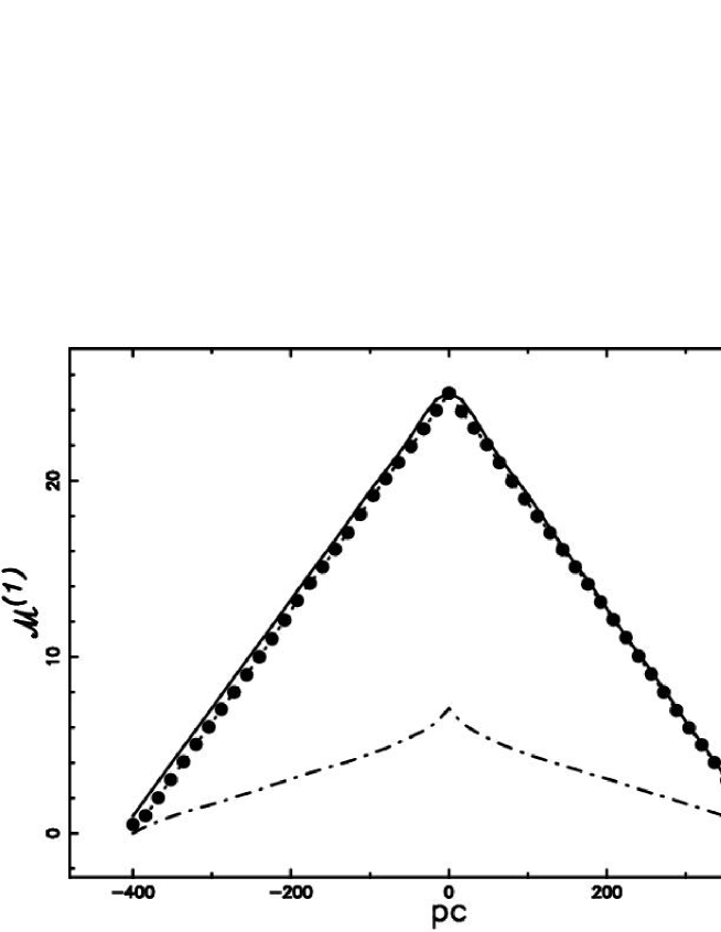
Figure 7: Profile of ${\mathcal{M}}^{(1)}$ versus the distance from the Galactic plane as given by Monte Carlo simulation with regular lengths step + theoretical results given by equation (34) + Monte Carlo simulation with Levy random walk (filled circles , dotted line and dot-dash-dot-dash line respectively ). The parameters are NDIM=51 , L=25, $m$ ranging from $1$ to $20$, side =800 pc , NTRIALS=10000 and $\alpha$=1.8 .

The effect of increasing the exponent $\alpha$ that regulates the lengths of the steps could be summarised in Figure 8 in which we report the value of the memory grid ${\mathcal{M}}^{(1)}$ at the center of the grid. From the previous figure is also clear the transition from Brownian motion ($\alpha\approx 2$ ) to regular motion ($\alpha\approx 10$ ).

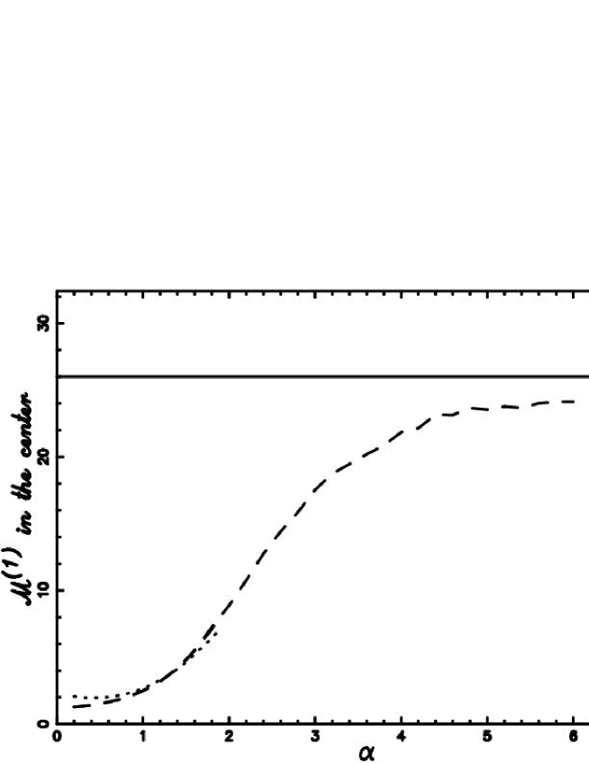
Figure 8: Behaviour of ${\mathcal{M}}^{(1)}$ at the center of the lattice as a function of $\alpha$ (dashed–line) + theoretical solution (dotted–line) + asymptotic behaviour at (NDIM+1)/2 (full line). Parameters as in Figure 7 .

2.6 Levy diffusion coefficient in 1D

The 1D diffusion coefficient in presence of Levy flights can be derived from analytical or numerical arguments that originate four different definitions summarised in Figure 9.

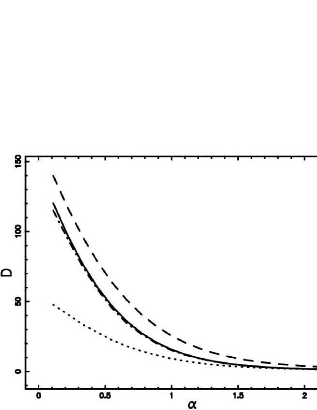
Figure 9: Behaviour of the diffusion coefficient as function $\alpha$: $D_{theo}^{I}$ ( full line ), $D_{theo}^{II}$ ( dashed ), $D_{num}^{I}$ ( dot-dash-dot-dash ), $D_{num}^{II}$( dotted ).

Let the single displacement,$\delta x$, be defined by

$$\delta x=\xi l,$$ (50)

where $l>0$ is the length of the flight and $\xi$ is a discrete random variable characterised by the following probabilities p(1)=+1 and p(2) =-1. The probability $p(\delta x)$ of a single displacement $\delta x$ is

$$p(\delta x)=\frac{1}{2}p(l)\quad.$$ (51)

This is the product of the probability $p(\xi)=1/2$ to go at right or at left by the probability $p(l)$ to make a step of length $l$. From $\langle\delta x\rangle=0$ and from the independence of the little steps follows

$$\langle x(n)\rangle=n\langle\delta x\rangle=0\quad,$$ (52)

where $x(n)$ is the walker’s position at the time $n$ ( after $n$ steps). From $\langle\delta x\rangle=0$ follows

$$\langle\delta^{2}x\rangle=\sigma^{2}(\delta x),\quad\langle x^{2}(n)\rangle=\sigma^{2}(x(n)),$$ (53)

and due to the independence of the small steps ,

$$\sigma^{2}(x(n))=n\sigma^{2}(\delta x)\quad.$$ (54)

The connection with the diffusion coefficient is through the theoretical relationship

$$D=\frac{1}{2}\sigma^{2}(\delta x),$$ (55)

thus

$$D=\frac{1}{2n}\sigma^{2}(x)\quad.$$ (56)

This formula can be compared with the well known formula that can be found on the textbooks , see for example formula (12.5) in [13]. We should now compute $\sigma^{2}(\delta x)$. Since $\langle\delta x\rangle=0$ and $\xi$, $l$ are random independent variables we have

$$\sigma^{2}(\delta x)=\langle\delta^{2}x\rangle=\langle(\xi l)^{2}\rangle=\langle\xi^{2}\rangle\langle l^{2}\rangle\quad.$$ (57)

Since $\langle\xi^{2}\rangle=1$

$$\sigma^{2}(\delta x)=\langle l^{2}\rangle\quad.$$ (58)

We can continue in two ways . A first one consists into evaluate $l^{2}$ according to the discrete distribution represented by equation (49). This originates the first theoretical diffusion coefficient , in the following $D_{theo}^{I}$. A second way consists into evaluate $\langle l^{2}\rangle$ in view of pdf (46)

$$\langle l^{2}\rangle=-{\frac{\alpha\,\left(-{{\it l_{max}}}^{\alpha}+{{\it l_{max}}}^{2}\right)}{\left({{\it l_{max}}}^{\alpha}-1\right)\left(-2+\alpha\right)}}\quad,$$ (59)

and consequently ,

$$D_{theo}^{II}=1/2\,{\frac{\alpha\,\left({{\it l_{max}}}^{\alpha}-{{\it l_{max}}}^{2}\right)}{\left({{\it l_{max}}}^{\alpha}-1\right)\left(-2+\alpha\right)}}\quad,$$ (60)

where the new $D_{theo}^{II}$ is the second theoretical diffusion coefficient.

The numerical techniques allow to implement two different definitions of the diffusion coefficient. The first one considers an infinite lattice and a variable number of Monte Carlo steps N (30,31…35) each one connected with an index j. The diffusion coefficient in then computed as :

$$D_{num}^{I}=\frac{\sum_{i=1}^{6}{\frac{R(i)^{2}}{2N(i)}}}{6}\quad.$$ (61)

The second evaluation implements a typical Monte Carlo run on a lattice , see for example the data in Figure 7. Now $R^{2}$ is fixed and takes the value $\frac{NDIM+1}{2}$ in contrast with N , the number of iterations before to reach the two boundaries, that is different in each run. We therefore have

$$D_{num}^{II}=\frac{R^{2}}{2\overline{N}}\quad,$$ (62)

where $\overline{N}$ is the average number of iterations necessary to reach the external boundary in each trial. Up to now in order to test the value of the diffusion coefficient we have fixed in one the minimum value that the step can take. We now explore the case in which the minimum length in pdf (46) is $l_{min}$ . On adopting the same technique that has lead to deduce $D_{theo}^{II}$ we obtain a new more general expression , $D_{theo}^{II,G}$ , for the 1D diffusion coefficient

$$D_{theo}^{II,G}=-1/2\,{\frac{\alpha\,\left({l_{{\min}}}^{2}{l_{{\max}}}^{\alpha}-{l_{{\max}}}^{2}{l_{{\min}}}^{\alpha}\right)}{\left(\alpha-2\right)\left(-{l_{{\max}}}^{\alpha}+{l_{{\min}}}^{\alpha}\right)}}\quad,$$ (63)

or introducing the ratio $r_{l}$ = $\frac{l_{min}}{l_{max}}$

$$D_{theo}^{II,G}=1/2\,{\frac{\alpha\,{l_{{\max}}}^{2}\left(-{r_{{l}}}^{2}+{r_{{l}}}^{\alpha}\right)}{\left(\alpha-2\right)\left(-1+{r_{{l}}}^{\alpha}\right)}}\quad.$$ (64)

3 Energy evaluations

In order to introduce the physical mean free path we should remember that an important reference quantity is the relativistic ions gyro-radius, $\rho_{Z}$. Once the energy is expressed in $10^{15}$eV units ( $E_{15}$) , and the magnetic field in $10^{-6}$ Gauss ( $H_{-6}$) we have:

$$\rho_{Z}=1.08\frac{E_{15}}{H_{-6}Z}pc\quad,$$ (65)

where Z is the atomic number. The solutions of the mathematical diffusion in presence of the steady state do not require the concept of mean free path. The solutions of the diffusion equation trough a Fourier expansion, Levy flights and Monte Carlo methods conversely require that the mean free path should be specified like a fraction of the size of the box in which the phenomena is analysed . The presence of irregularities allows the diffusion of the charged particles. The mean free path $\lambda_{sc}$ , see for example  [12] , is

$$\lambda_{sc}\approx\rho_{Z}\Phi^{-2}\quad,$$ (66)

with $\Phi=\frac{B_{1}}{B_{0}}$ where ${B_{1}}$ are ${B_{0}}$ are the strength of the random and mean magnetic field respectively. The type of adopted turbulence, weak or strong, the spectral index of the turbulence determine the exact correspondence between energy and mean free path. Some evaluations on the relativistic mean free path of cosmic rays and Larmor radius can be found in [12, 25, 26, 27]. The transport of cosmic rays with the length of the step equal to the relativistic ion gyro-radius is called Bohm diffusion [28] and the diffusion coefficient will be energy dependent. The assumption of the Bohm diffusion allows to fix a one-to-one correspondence between energy and length of the step of the random walk. The presence of a short wavelength drift instability in the case of quasi-perpendicular shocks drives the diffusion coefficient to the ”Bohm” limit [29, 30]. The maximum energies that can be extracted from SNR and Super-bubbles are now introduced. The transit times in the halo of our galaxy are computed in the case of a fixed and variable magnetic field. The modification of the canonical energy probability density function , p(E) $\propto~{}E^{-2}$, due to an energy dependent diffusion coefficient is outlined.

3.1 Maximum available energies

The maximum energy available in the accelerating regions is connected with their size, in the following $\Delta~{}R$ and with the Bohm diffusion

$$\Delta~{}R=\rho_{Z}\quad.$$ (67)

The most promising sites are the SNR as well as the super-shell. In the case of SNR, the analytical solution for the radius can be found in [31] (equation 10.27) :

$$R(t)=\left(\frac{25E^{expl}t_{SNR}^{2}}{4\pi\rho_{0}}\right)^{1/5}\quad,$$ (68)

where $\rho_{0}$ is the density of the surrounding medium supposed to be constant , $E^{expl}$ is the energy of the explosion, and $t_{SNR}$ is the age of the SNR. Equation (68) can be expressed by adopting the astrophysical units

$$R=(\frac{E_{51}^{expl}t_{4}^{2}}{n_{0}})^{1/5}12.47\mathrm{pc}\quad,$$ (69)

here $t_{4}$ is $t_{\mathrm{SNR}}$ expressed in units of $10^{4}$ years, $E_{51}^{expl}$ is the energy expressed in units of $10^{51}$ ergs and $n_{0}$ is the density expressed in $\mathrm{particles~{}}$ ${\mathrm{cm}^{-3}}$ . In agreement with [31] $\rho_{0}$ = $n_{0}$ m was taken, where m = 1.4 $m_{H}$ : this energy conserving phase ends at $t_{4}\approx 1.4$. The thickness of the advancing layer is $\Delta~{}R$ $\approx$ $R/12$ according to [31] and this allows us to deduce the maximum energy ,$E^{max}_{15}$, that can be extracted from SNR for a relativistic ion , see formula (67):

$$E^{max}_{15}=0.961\bigl{(}\frac{E_{51}^{expl}t_{4}^{2}}{n_{0}}\bigr{)}^{1/5}H_{-6}Z\quad.$$ (70)

This new formula is in agreement with more detailed evaluations [32].

The super-shells have been observed as expanding shells, or holes, in the H I-column density distribution of our galaxy [33]. The dimensions of these objects span from 100 pc to 1700 pc and often present elliptical shapes or elongated features, that can be explained as an expansion in a non-homogeneous medium [34]. An explanation of the super-shell is obtained from the theory of the Superbubbles , in the following SB, whose radius is  [31]

$$R=\left[\frac{25}{14\pi}\right]^{1/5}\left(\frac{E_{0}R_{\mathrm{SN}}}{{\rho}}\right)^{1/5}t^{3/5},$$ (71)

where t is the considered time, $R_{\mathrm{SN}}$ is the rate of supernova explosions, and $E_{0}$ the energy of each supernova; this equation should be considered valid only if the altitude of the OB associations from the Galactic ,$z_{OB}$=0, is zero, and only for propagation along the Galactic plane.

When the astrophysical units are adopted the following is found

$$R=111.56\;\mathrm{pc}(\frac{E_{51}^{expl}t_{7}^{3}N^{*}}{n_{0}})^{\frac{1}{5}},$$ (72)

where $t_{7}$ is the time expressed in $10^{7}$ yr units, $E_{51}^{expl}$ is the energy in $10^{51}$ erg, $n_{0}$ is the density expressed in particles $\mathrm{cm}^{-3}$, and $N^{*}$ is the number of SN explosions in $5.0\cdot 10^{7}$ yr. As an example, on inserting in equation (72) the typical parameters of GSH 238 [33] , $E_{51}^{expl}$=1 , $t_{7}$=2.1 , $n_{0}$=1 and $N^{*}$=80.9 , the radius turns out to be 419 pc in rough agreement with the average radius of GSH 238 , $\approx$ 385 pc.

The maximum energy ,$E^{max,sb}_{15}$, that can be extracted from a SB ( from formula (67)) in the Bohm diffusion is therefore:

$$E^{max,sb}_{15}=8.61\bigl{(}\frac{E_{51}^{expl}N^{*}}{n_{0}}\bigr{)}^{1/5}t_{7}^{3/5}H_{-6}Z\quad.$$ (73)

Once the typical parameters of GSH 238 are inserted in equation (73) we obtain $E^{max,sb}_{15}=323.6~{}H_{-6}~{}Z$. The exact value of the magnetic field in the expanding layer of the SB is still subject of research , the interval $H_{-6}~{}\in\{1,...200\}$ being generally accepted [35]. The interested reader can compare our equation (73) with equation (15) in [35].

3.2 Transit times

The absence of the isotope $~{}^{10}Be$, which has a characteristic lifetime $\tau_{r}=0.39\times 10^{7}~{}yr$ , implies the following inequality on $\tau$, the mean cosmic ray residence time ,

$$\tau>\tau_{r}\quad.$$ (74)

Given a box of side L with a proton inserted at the center, the classical time of crossing the box $t_{c}$ is :

$$t_{c}=\frac{L}{2c}\quad.$$ (75)

Once the pc and yr units are chosen , $c=0.306\frac{pc}{yr}$ and

$$t_{c}=1.63L_{1}~{}yr\quad,$$ (76)

where $L_{1}$ is the side of the box expressed in 1pc units.

When the side of the box is $L_{1}$=800, $t_{c}\approx 1304~{}yr$, and $t_{c}\ll\tau_{r}$, we should discard the diffusion of the cosmic rays through the ballistic model.

We now analyse firstly the case in which the value of the diffusion coefficient is constant and secondly the case in which the diffusion coefficient is variable.

3.2.1 Transit times when D is fixed

From equations (3) and (8) we easily find the time , t, necessary to travel the distance R

$$t=\frac{R^{2}}{c_{tr}c\lambda}\quad,$$ (77)

where $v_{tr}=c_{tr}~{}c$ . We continue inserting $R=\frac{L}{2}$ , $L=L_{1}~{}pc$ and $t=t_{1}~{}10^{7}~{}yr$ ,

$$t_{1}=0.815\times 10^{-7}\frac{L_{1}^{2}}{c_{tr}\lambda_{1}}\quad.$$ (78)

Figure 10 reports a plot of the transit times versus the two main parameters $\lambda_{1}$ and $c_{tr}$ together with the constrains represented by the lifetime of the $~{}^{10}Be$. In this case the lifetime of the phenomena ( cross-hatched region ) is tentatively fixed in $t_{1}=10$.

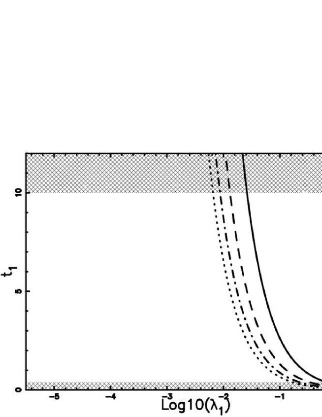
Figure 10: Transit times expressed in $10^{7}$ yr units as a function $\lambda_{1}$ when $L_{1}$=800 : $c_{tr}=0.2$ ( full line), $c_{tr}=0.4$ ( dashed), $c_{tr}=0.6$ ( dot-dash-dot-dash), $c_{tr}=0.8$ ( dotted). The forbidden region is represented through cross-hatched lines.

Conversely in presence of Levy flights (diffusion coefficient as given by formula 64) the transit time $t_{1}^{L}$ takes the form

$$t_{1}^{L}=-0.815\times 10^{-7}\frac{L_{1}^{2}}{c_{tr}\lambda_{1}}{\frac{\left(\alpha-2\right)\left(-1+{r_{{l}}}^{\alpha}\right)}{\alpha\,\left({r_{{l}}}^{2}-{r_{{l}}}^{\alpha}\right)}}\quad.$$ (79)

The effect of the Levy flights is to increase the value of the transit times. Is interesting to realize that, in this astrophysical form of the Levy flights, the steps with transport velocity greater than the light velocity are avoided.

3.2.2 Transit times when D is variable

The value of the pressure in the Solar surroundings takes the value , $p_{12}10^{-12}{\mathrm{dyne~{}cm}}^{-2}$ [36] when the pressure is expressed in $10^{-12}{\mathrm{dyne~{}cm}}^{-2}$ units , $p_{12}$.

Assuming equipartition between thermal pressure and magnetic pressure, the magnetic field $B_{0}$ at the Galactic plane turns out to be

$$B_{0}=\sqrt{5}10^{-6}{p_{12}}~{}Gauss\quad.$$ (80)

The behaviour of the magnetic field with the Galactic height z in pc is assumed to vary as

$$B=\frac{B_{0}}{1+a_{D}z}\quad,$$ (81)

with $D_{0}$ defined in Section 2.3.4 through the Bohm diffusion ,

$$D_{0}=\frac{1}{d}c_{tr}\frac{E_{15}}{H_{-6}Z}0.166~{}10^{7}~{}~{}\frac{pc^{2}}{(10^{7}yr)}\quad.$$ (82)

In order to see how the presence of a variable diffusion coefficient modifies the transit times given by equation (78) we performed the following Monte Carlo simulation. The 1D random walk has now the length of the step function of the distance from the origin. In order to mimic equation (28) the step has length

$$\lambda=\lambda 1(1+a_{D}z)\quad.$$ (83)

Typical behaviour of the influence of the variable D on transit times has been reported in Figure 11.

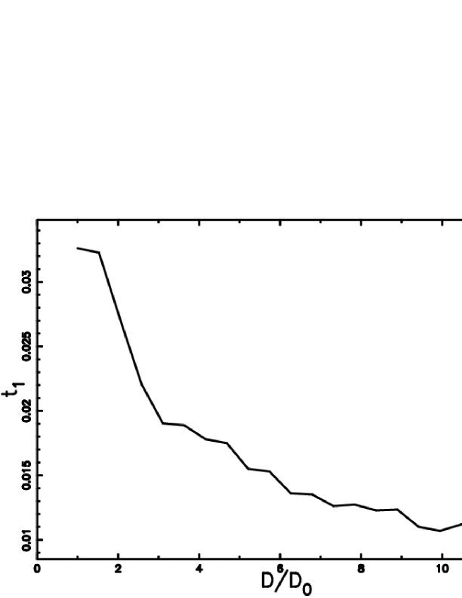
Figure 11: Transit times expressed in $10^{7}$ yr units as a function of $D(400pc)/D(0)=10$ when $L_{1}$=800, $\lambda_{1}$=8 and $c_{tr}=0.2$. Assuming Z=1 ,$H_{-6}$=1 we have ( Bohm diffusion) $E_{15}$=7.38

It is clear that an increasing D ( a decreasing B) lowers the transit times; a rough evaluation predicts that transit times decrease $\propto~{}D(400pc)/D(0)$.

3.3 The spectral index

At present the observed differential spectrum of cosmic rays scale as $E^{-2.75}$ in the interval $10^{10}~{}eV-5.0~{}10^{15}~{}eV$ and after $5~{}10^{15}~{}eV$ as $E^{-3.07}$.

Up to now the more interesting result on the prediction of the spectral index resulting from particle acceleration in shocks , i.e. SNR or SB , is due to [37, 38, 12].

The predicted differential energy spectrum of the high energy protons is

$$N(E)dE\propto E^{-2}dE\quad.$$ (84)

This is the spectral index where the protons are accelerated ; i.e. the region that has size $\approx~{}\frac{R}{12}$ , where R is the radius of the SNR or SB. Due to the spatial diffusion, the spectral index changes. The first assumption is that the transport occurs at lengths of the order of magnitude of the gyro-radius, the previously introduced Bohm diffusion. Two methods are now suggested for the modification of the original index as due to the diffusion : one deals with the concept of advancing segment/circle or sphere and the second one is connected with the asymptotic behaviour of the 3D concentration.

3.3.1 Index from the diffusion coefficient

On considering a diffusion function of the dimensionality d (see formula (3)) , the square of the distances in presence of Bohm diffusion will be

$${\overline{R}^{2}}=\frac{0.3310^{7}c_{tr}E_{15}t_{1}}{H_{-6}Z}~{}pc^{2}\quad.$$ (85)

Let us consider two energies $E_{15,1}$ and $E_{15,2}$ with two corresponding numbers of protons (Z=1) , $N_{1}$ and $N_{2}$. We have two expressions for the two advancing spheres (d=3) characterised by radius $R_{1}(E_{15,1})$ and $R_{2}(E_{15,2})$.

The ratio of the two densities per unit volume , $N_{2,1}$, gives the differential spectrum

$$N_{2,1}=\frac{\rho_{1}}{\rho_{2}}=\frac{N_{2}}{N_{1}}(\frac{E_{15,1}}{E_{15,2}})^{3/2}\quad.$$ (86)

But in the source

$$\frac{N_{2}}{N_{1}}=(\frac{E_{15,1}}{E_{15,2}})^{2}\quad,$$ (87)

and therefore

$$N_{2,1}\propto(\frac{E_{15,1}}{E_{15,2}})^{3.5}\quad or\propto E^{-3.5}\quad,$$ (88)

when d=3 or

$$N_{2,1}\propto E^{-(2+d/2)}\quad,$$ (89)

when the concentration is function of d. This new demonstration simply deals with the concept of advancing segment/circle or sphere.

3.3.2 Index from the 3D concentration

Starting from the asymptotic behaviour of the 3D concentration , formula (18) the ratio of the two energy concentrations is possible to derive a new formula

$$N_{2,1}\propto E^{-(2+1)}\quad.$$ (90)

4 CR Diffusion in the SB environment

Once equipped to calculate the spatial diffusion and temporal evolution of the CR attention now moves to the 3D evolution of CR once they have been accelerated in the advancing layer of super-shells.

4.1 SB

The super-shells have been observed as expanding shells, or holes, in the H I-column density distribution of our galaxy and the dimensions of these objects span from 100 pc to 1700 pc [39]. The elongated shape of these structures is explained through introducing theoretical objects named super-bubble (SB); these are created by mechanical energy input from stars [40, 41, 31].

The evolution of the SB’s in the ISM can be followed once the following parameters are introduced $t_{\mathrm{\mathrm{age}}}$ , the age of the SB in yr, $\Delta t$, the time step to be inserted in the differential equations, $t^{\mathrm{burst}}$, the time after which the bursting phenomena stops , $N^{*}$, which is the number of SN explosions in $5.0\cdot 10^{7}$ yr. An analytical solution of the advancing radius as a function of time can be found [31] when the ISM has constant density.

The basic equation that governs the evolution of the SB [31], [42] is momentum conservation applied to a pyramidal section, characterised by a solid angle, $\Delta\Omega_{j}$:

$$\frac{d}{dt}\left(\Delta M_{j}\dot{R}_{j}\right)=pR_{j}^{2}\Delta\Omega_{j},$$ (91)

where $\Delta\Omega_{j}$ is the solid angle along a given direction and the mass is confined into a thin shell with mass $\Delta M_{j}$. The subscript $j$ indicates that this is not a spherically symmetric system.

In our case the density is given by the sum of three exponentials

$$n(z)=n_{1}e^{-z^{2}/{H_{1}}^{2}}+n_{2}e^{-z^{2}/{H_{2}}^{2}}+n_{3}e^{-|z|/{H_{3}}}\,,$$ (92)

where z is the distance from the Galactic plane in pc, $n_{1}$=0.395 ${\mathrm{particles~{}}}{\mathrm{cm}^{-3}}$, $H_{1}$=127 pc, $n_{2}$=0.107 $\mathrm{particles~{}}{\mathrm{cm}^{-3}}$, $H_{2}$=318 pc, $n_{3}$=0.064 $\mathrm{particles~{}}{\mathrm{cm}^{-3}}$, and $H_{3}$=403 pc and this requires that the differential equations should be solved along a given number of directions each denoted by $j$ . By varying the basic parameters, which are the bursting time and the lifetime of the source characteristic structures such as hourglass-shapes, vertical walls and V-shapes, can be obtained. The SB are then disposed on a spiral structure as given by the percolation theory and the details can be found in [34].

The influence of the Galactic rotation on the results can be be obtained by introducing the law of the Galactic rotation as given by [43],

$$V_{\mathrm{R}}(R_{0})=220(\frac{R_{0}[\mathrm{pc}]}{8500})^{0.382}\mathrm{km~{}sec}^{-1},$$ (93)

here $R_{0}$ is the radial distance from the center of the Galaxy expressed in pc. The original circular shape of the superbubble at z=0 transforms in an ellipse through the following transformation, $T_{\mathrm{r}}$,

$$T_{\mathrm{r}}~{}\left\{\begin{array}[]{l}x\prime=x+0.264y~{}t\\ \vskip 6.0pt plus 2.0pt minus 2.0pt\cr y\prime=y\\ \vskip 6.0pt plus 2.0pt minus 2.0pt\cr z\prime=z,\end{array}\right.$$ (94)

where y is expressed in pc and t in $10^{7}~{}{\mathrm{yr}}$ units [34]. In the same way the effect of the shear velocity as function of the distance y from the center of the expansion, $V_{shift}(y)$ can be easily obtained on Taylor expanding equation (93)

$$V_{shift}(y)=84.04\frac{y}{R_{0}}\,Km/s\quad.$$ (95)

This is the amount of the shear velocity function of y but directed toward x in a framework in which the velocity at the center of the expansion is zero and is new.

4.2 Monte Carlo diffusion of CR from SB

The diffusing algorithm here adopted is the 3D random walk from many injection points ( in the following IP), disposed on $N_{SB}$ super-bubbles. In this case a time dependent situation is explored ; this is because the diffusion from the sources cannot be greater than the lifetime of SB. The rules are :

1. The first of $N_{SB}$ SB is chosen.

2. The IP are generated on the surface of each SB.

3. The 3D random walk starts from each IP with a fixed length of a step. The number of visits is recorded on a 3D grid $\mathcal{M}$ .

4. After a given number of iteration , ITMAX , the process restarts from (iii) taking into account another IP.

5. After the diffusion from the n SB , the process restarts from (i) and the (n+1) SB is considered.

The spatial displacement of the 3D grid ${\mathcal{M}}({i,j,k})$ can be visualised through the ISO-density contours. In order to do so, the maximum value ${{\mathcal{M}}(i,j,k)}_{max}$ and the minimum value ${{\mathcal{M}}({i,j,k})}_{min}$  should be extracted from the three-dimensional grid. A value of the visitation or concentration grid can then be fixed by using the following equation:

$${{\mathcal{M}}({i,j,k})}_{chosen}={{\mathcal{M}}({i,j,k})}_{min}+{({{{\mathcal{M}}({i,j,k})}_{max}-{{\mathcal{M}}({i,j,k})}_{min}})\times{coef}}\quad,$$ (96)

where coef is a parameter comprised between 0 and 1. This iso-surface rendering is reported in Fig 12  ; the Euler angles characterising the point of view of the observer are also reported .

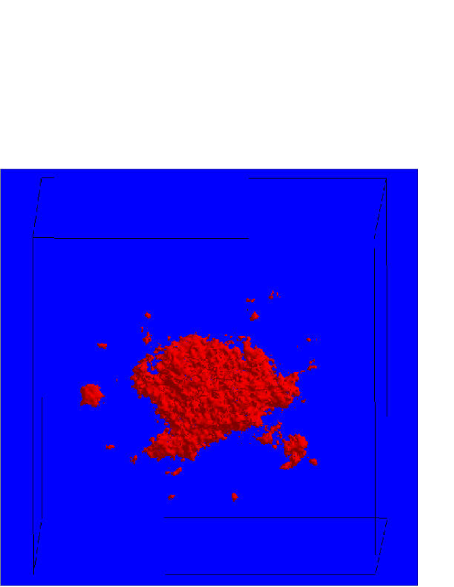
Figure 12: Three dimensional surface representing the surface brightness, front view. The ISO–density contours are fixed through coef=0.55. The number of super-bubbles $N_{SB}$ is 260 and the time evolution is followed as in [34] , $\lambda_{1}$=172.94, IP=200 , ITMAX= 20000 , $t_{D}~{}=2.26~{}10^{7}$ yr and $c_{tr}=0.5$. Assuming Z=1 ,$H_{-6}$=1 we have ( Bohm diffusion) $E_{15}$=159.68 .

From the previous figure it is possible to see a progressive intersection of the contributions from different super-bubbles: once we decrease ITMAX , the spiral structure of spatial distribution of SB is more evident , see Figure 13 .

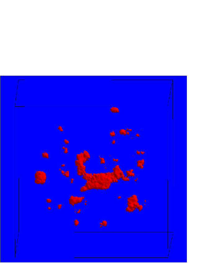
Figure 13: The same as Figure 13 but ITMAX= 600 , $t_{D}~{}=6.7~{}10^{5}$, and coef=0.40.

The results can also be visualised through a 2D grid representing the concentration of CR along the Galactic plane x-y , see Figure 14, or 1D cut , see Figure 15 .

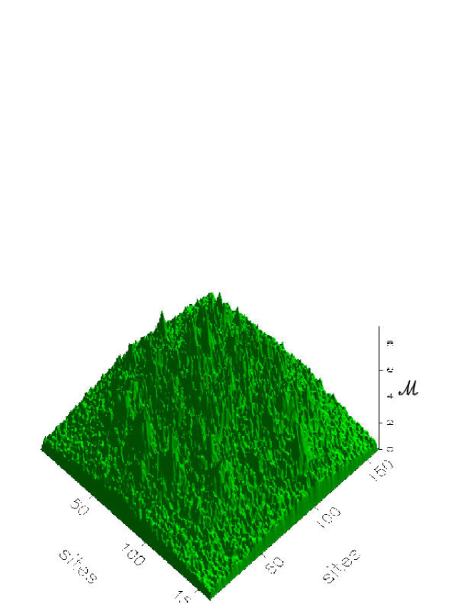
Figure 14: Concentration of CR at the x-y (z=0) Galactic plane. Data as in Figure 12.

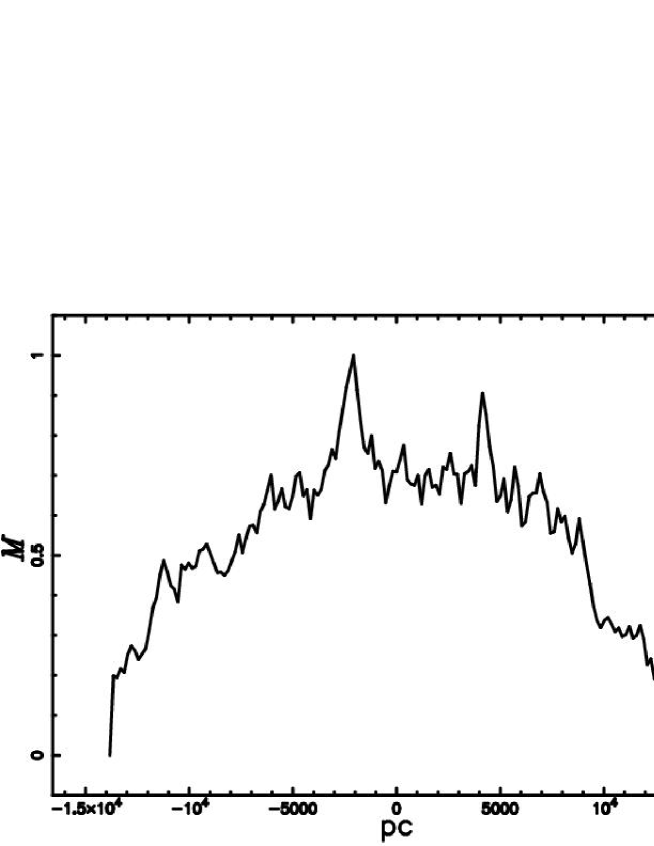
Figure 15: Cut along the Galactic plane , x-y, of the concentration of CR crossing the center. Data as in Figure 12.

From this figure the contribution from the SB belonging to the arms is clear ; this profile should be a flat line when the mathematical diffusion is considered. Another interesting case is the cut along the Galactic height z , see Figure 16.

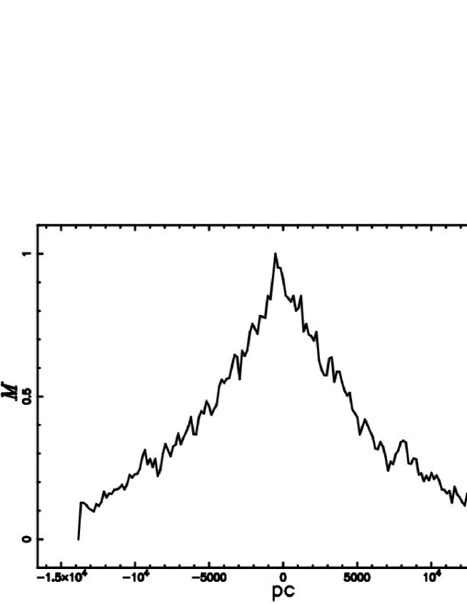
Figure 16: Cut of the concentration of CR along a direction perpendicular to the Galactic plane and crossing the center. Data as in Figure 12.

from which the irregularities coming from the position of the SB on the arms are visible; this profile should have a triangular shape when the 1D mathematical diffusion from the Galactic plane is considered.

4.3 The gamma emission from the Galactic plane

The cosmic rays with an energy range $0.1~{}GeV<E<410^{5}GeV$ [44, 45] can produce gamma ray emission ( $30MeV<E<30GeV$) from the interaction with the target material [45, 44, 46]. The gamma ray emissivity will therefore be proportional to the concentration of CR.

A typical map of $\gamma$-emission from the Galactic plane is visualised in Figure 17 , where the additive property of the intensity of radiation along the line of sight is applied. Using the algorithm of the nearest IP [47] it is also possible to visualise the $\gamma$-emission in the Hammer-Aitof projection,see Figure 18.

Figure 17: Intensity of the gamma-rays along the line of sight when the galaxy is face on. The parameters of the diffusion are Z=1 , $t_{D}~{}=0.6~{}10^{7}$yr , $c_{tr}=0.5$ , $H_{-6}$=1 , $\lambda_{1}$=9.22

and ( Bohm diffusion) $E=8.5~{}10^{6}~{}GeV$ .

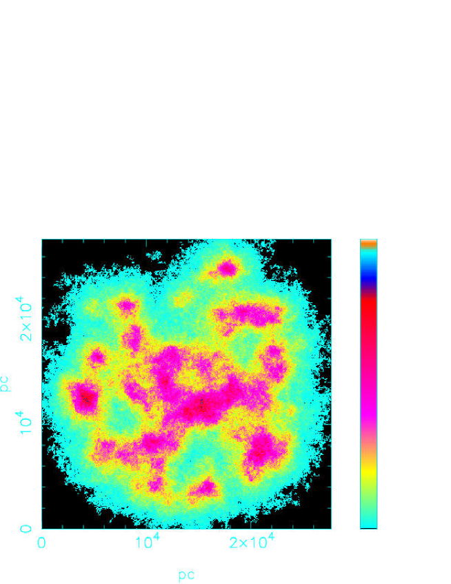
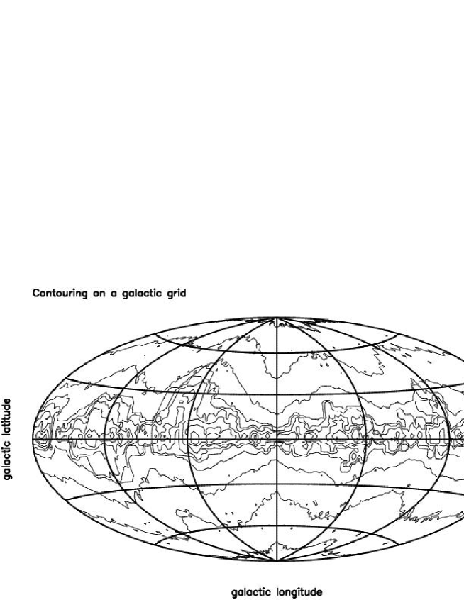
Figure 18: Intensity of the gamma-rays along the line of sight in the Hammer-Aitof projection. The parameters are the same of Figure 17.

The observations with EGRET [46] provide cuts in the intensity of radiation that can be interpreted in the framework of the random walk. We therefore report in Figure 19 the behaviour of the intensity of the gamma ray emission proportional to concentration of CR when the distance from the Galactic plane is expressed in Galactic latitude; in the figure the stars represent the plot $(30^{\circ}>l>10^{\circ})$ of [46].

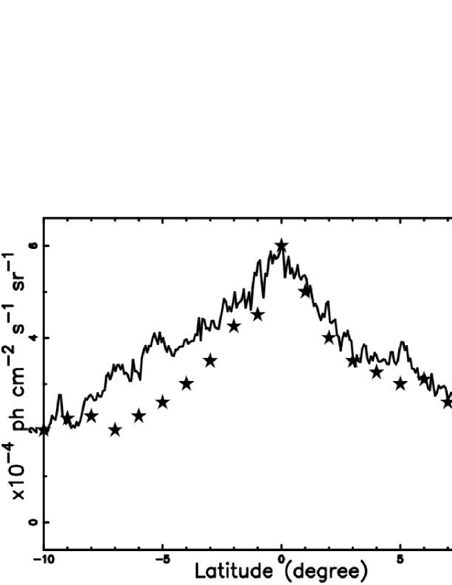
Figure 19: Theoretical gamma-ray emission as given by Monte Carlo simulation as function of the Galactic latitude when the cut is crossing the center and the observer is at 700 pc, data as in Figure 17. The stars represent the observational cut.

4.4 Monte Carlo diffusion of CR from the Gould Belt

The physical parameters concerning the Gould Belt as deduced in [48], are reported in Table 1.

Table 1: Data of the super-shell associated with the Gould Belt

$$\begin{array}[]{cc}\hline\cr\vskip 3.0pt plus 1.0pt minus 1.0pt\cr\mbox{Size (pc}^{2})&466\cdot 746\mbox{~{}at~{}b=0}\\ \mbox{Expansion~{}velocity~{}(km~{}s}^{-1})&17\\ \mbox{Age~{}(10}^{7}\,{\mathrm{yr}})&2.6\\ \mbox{Total energy~{}\,(10}^{51}{\mathrm{erg}})&6\\ \vskip 3.0pt plus 1.0pt minus 1.0pt\cr\hline\cr\end{array}$$

The total energy is such as to produce results comparable with the observations and the kinematic age is the same as in [48]. In order to obtain $E_{\mathrm{tot}}=6.~{}10^{51}{\mathrm{erg}}$ with $t^{\mathrm{burst}}=0.015~{}10^{7}~{}{\mathrm{yr}}$, we have inserted $N^{*}$= 2000. The time necessary to cross the Earth orbit , that lies 104 pc away from the Belt center, turns out to be $0.078~{}10^{7}~{}yr$ that means $2.52~{}10^{7}~{}yr$ from now. The 2D cut at z=0 of the superbubble can be visualised in Figure 20.

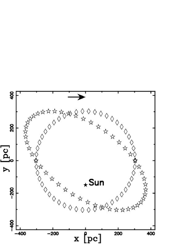
Figure 20: Rhombi represent the circular section, the stars the rotation-distorted section and the big star the Sun. The Galaxy direction of rotation is also shown. The parameters are $t_{\mathrm{\mathrm{age}}}$=$2.6\cdot 10^{7}~{}\mathrm{yr}$, $\Delta$ $t=0.001\cdot 10^{7}~{}\mathrm{yr}$, $t^{\mathrm{burst}}_{7}$= 0.015, $N^{*}$= 2000, $z_{\mathrm{OB}}$=0 pc, and $E_{51}$=1.

Our model gives a radial velocity at z =0 $V_{\mathrm{theo}}$=3.67 $\mbox{km~{}s}^{-1}$. The influence of the Galactic rotation on the direction and modulus of the field of originally radial velocity the transformation (95) is applied , see Figure 21. A comparison should be done with Figure 5 and Figure 9 in [48].

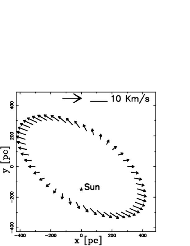
Figure 21: The stars represents the rotation-distorted section of the Gould Belt and the big star the Sun. The velocity field of the expansion modified by the shear velocity is mapped. The Galaxy direction of rotation is also shown.

The results of the streaming of CR from the complex 3D advancing surface of the Gould Belt can be visualized through a 2D grid representing the concentration of CR along the Galactic plane x-y (z=0) , see Figure 22, or through a perpendicular plane x-z (y=0), see Figure 23.

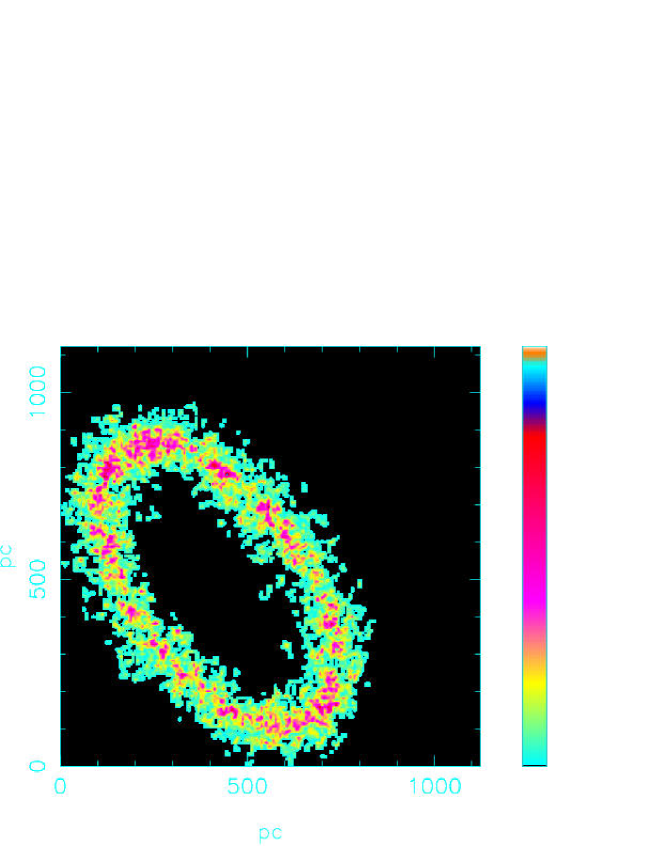
Figure 22: Concentration of CR diffusing away from the Gould Belt at the x-y (z=0) plane. $\lambda_{1}$=5.51, IP=10000 , ITMAX= 200 , $t_{D}~{}=~{}7204$ yr and $c_{tr}=0.5$. Assuming Z=1 ,$H_{-6}$=1 we have ( Bohm diffusion) $E_{15}$=5.08 .

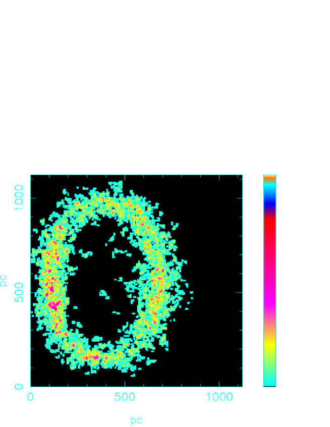
Figure 23: The same as Figure 23 but in the x-z (y=0) plane.

The variation of CR due to the presence of the Gould Belt are also analyzed in Section 3.2 in [7].

5 Conclusions

We have studied the propagation of CR with the aid of mathematical diffusion in 1D, 2D and 3D. Due to the nature of the problem , diffusion from the Galactic plane , the first results can be obtained in 1D. The 1D diffusion has also been analysed in the case of a variable diffusion coefficient: which in our astrophysical case consists in a magnetic field function of the altitude z from the Galactic plane. These analytical results allow to test the Monte Carlo diffusion. The physical explanation is the diffusion through the Larmor radius which means that the diffusion coefficient depends on energy. The calculation of the transit times of CR explains the absence of the isotope $~{}^{10}Be$. Further on the theoretical and Monte Carlo set up of the Levy flights allows to increase the applications of the random walk. For example from an observed profile of CR function of distance from the Galactic plane is possible to evaluate the concavity: the 1D Levy flights predict profiles concave up and the 1D regular random walk predicts no concavity. The observations with EGRET in the gamma range , see Figure 3 in  [46] , provide profiles that are concave up and therefore the Levy flights with the shape regulating parameter $\alpha$ can be an explanation of the observed profiles, see Figure 7.

The CR diffusion in a super-bubble environment is then performed by evaluating the maximum energies that can be extracted ($\approx~{}10^{17}eV)$ and performing a Monte Carlo simulation of the propagation of CR from SB disposed on a spiral-arm network. According to the numerical results, the concentration of CR depends on the distance from the nearest SB and from the chosen energy.

This fact favours the local origin of CR [49] that comes out from an analysis of the results of KASCADE data [50]. From an astrophysical point of view, local origin means to model the diffusion from the nearest SNR or SB. Like a practical example we now explore the case of the Gould Belt, the nearest SB , which has an average distance of 300 $\approx$ pc from us. The concentration of CR at the source of this SB is , according to formula (18):

$$C_{{m}}\approx C(300)\frac{300~{}pc}{\rho_{Z}}\approx 277\times C(300)\frac{H_{-6}Z}{E_{15}}\quad,$$ (97)

where $C(300)$ is the measured concentration on Earth at the given energy. Is interesting to point out that the crossing time (25 My ago) of the expanding Gould Belt with the Earth with a consequent increases in the concentration of CR can explain one event of the fossil diversity cycle that has a periodicity of 62 My [51] . The gamma-ray emissivity is different in the various regions of the galaxy [52] , and in order to explain this fact the theoretical map of gamma-ray from the Galactic plane has been produced. CR with energies greater that $10^{18}eV$ , Ultra-High Energy (UHE) , are thought to be of extra-galactic origin ([27, 53, 54, 55, 56, 57]) and therefore the diffusion from extra-galactic sources through the intergalactic medium is demanded to a future investigation.

References

- [1] R. M. Kulsrud, Plasma physics for astrophysics, Princeton University Press, Princeton, N.J., 2005.
- [2] P. Sokolosky, Introduction to Ultrahigh Energy Cosmic Ray Physics, Westview Press, Boulder, CO, 2004.
- [3] R. Blandford, D. Eichler, Phys. Rep. 154 , 1(1987) .
- [4] A. W. Strong, I. V. Moskalenko, ApJ 509 , 212(1998) .
- [5] R. Taillet, D. Maurin, A&A 402 , 971(2003) .
- [6] R. E. Lingenfelter, Nature 224 , 1182(1969) .
- [7] I. Büsching, A. Kopp, M. Pohl, R. Schlickeiser, C. Perrot, I. Grenier, ApJ 619 , 314(2005) .
- [8] A. D. Erlykin, A. W. Wolfendale, Astroparticle Physics 25 , 183(2006) .
- [9] W. R. Binns, M. E. Wiedenbeck, M. Arnould, A. C. Cummings, J. S. George, S. Goriely, M. H. Israel, R. A. Leske, R. A. Mewaldt, G. Meynet, L. M. Scott, E. C. Stone, T. T. von Rosenvinge, ApJ 634 , 351(2005) .
- [10] J. C. Higdon, R. E. Lingenfelter, ApJ 628 , 738(2005) .
- [11] J. C. Higdon, R. E. Lingenfelter, ApJ 590 , 822(2003) .
- [12] M. S. Longair, High energy astrophysics, Cambridge University Press, 2nd ed., Cambridge, 1994.
- [13] H. Gould, J. Tobochnik, An introduction to computer simulation methods, Addison-Wesley, Reading, Menlo Park, 1988.
- [14] H. C. Berg, Random Walks in Biology, Princeton University Press, Princeton, 1993.
- [15] J. Crank, Mathematics of Diffusion, Oxford University Press, Oxford, 1979.
- [16] R. M. Barrer, Proceedings of the Physical Society 58 , 321(1946) .
- [17] W. Feller, An Introduction to Probability Theory and Its Applications, John Wiley and Sons, New-York, 1966.
- [18] P. H. Morse , H. Feshbach, Methods of Theoretical Physics, McGraw-Hill, New-York, 1953.
- [19] M. Ferraro, L. Zaninetti, Physica A 338 , 307(2004) .
- [20] P. Levy , Theorie de l’Addition des Variables Aleatoires, Gauthier-Villars, Paris, 1937.
- [21] M. Gitterman, Phys. Rev. E 62 , 6065(2000) .
- [22] M. Evans, N. Hastings, P. B., Statistical Distributions - third edition, John Wiley & Sons Inc, New York, 2000.
- [23] S. Brandt, G. Gowan, Data Analysis: Statistical and Computational Methods for Scientists and Engineers, Springer & Verlag, New-York, 1998.
- [24] M. Ferraro, L. Zaninetti, Phys. Rev. E 73 (5) , 057102(2006) .
- [25] J. R. Jokipii, ARA&A 11 , 1(1973) .
- [26] D. G. Wentzel, ARA&A 12 , 71(1974) .
- [27] P. Bhattacharjee, G. Sigl, Phys. Rep. 327 , 109(2000) .
- [28] D. Bohm, E. Burhop, H. Massey, in Characteristic of Electrical Discharges in Magnetic Fields, McGraw-Hill, New-York, 1949.
- [29] G. P. Zank, W. I. Axford, J. F. McKenzie, A&A 233 , 275(1990) .
- [30] F. C. Jones, D. C. Ellison, Space Science Reviews 58 , 259(1991) .
- [31] A. McCray, R. In: Dalgarno, D. Layzer (Eds.), Spectroscopy of astrophysical plasmas, Cambridge University Press, 1987.
- [32] P. O. Lagage, C. J. Cesarsky, A&A 125 , 249(1983) .
- [33] C. Heiles, ApJ 498 , 689(1998) .
- [34] L. Zaninetti, PASJ 56 , 1067(2004) .
- [35] E. Parizot, A. Marcowith, E. van der Swaluw, A. M. Bykov, V. Tatischeff, A&A 424 , 747(2004) .
- [36] A. Boulares, D. P. Cox, ApJ 365 , 544(1990) .
- [37] A. R. Bell, MNRAS 182 , 443(1978) .
- [38] A. R. Bell, MNRAS 182 , 147(1978) .
- [39] C. Heiles, ApJ 229 , 533(1979) .
- [40] S. B. Pikel’Ner, Astrophys. Lett. 2 , 97(1968) .
- [41] R. Weaver, R. McCray, J. Castor, P. Shapiro, R. Moore, ApJ 218 , 377(1977) .
- [42] R. McCray, M. Kafatos, ApJ 317 , 190(1987) .
- [43] J. G. A. Wouterloot, J. Brand, W. B. Burton, K. K. Kwee, A&A 230 , 21(1990) .
- [44] A. M. Hillas, J. Phys. G 31 , 95(2005) .
- [45] A. W. Wolfendale, J. Phys. G 29 , 787(2003) .
- [46] S. D. Hunter, D. L. Bertsch, J. R. Catelli, T. M. e. a. Dame, ApJ 481 , 205(1997) .
- [47] L. Zaninetti, A&A 190 , 17(1988) .
- [48] C. A. Perrot, I. A. Grenier, A&A 404 , 519(2003) .
- [49] A. D. Erlykin, A. W. Wolfendale, Astroparticle Physics 23 , 1(2005) .
- [50] J. R. Hörandel, Astroparticle Physics 21 , 241(2004) .
- [51] M. V. Medvedev, A. L. Melott, ArXiv Astrophysics e-prints .
- [52] S. W. Digel, I. A. Grenier, S. D. Hunter, T. M. Dame, P. Thaddeus, ApJ 555 , 12(2001) .
- [53] K. Dolag, D. Grasso, V. Springel, I. Tkachev, Journal of Cosmology and Astro-Particle Physics 1 , 9(2005) .
- [54] D. DeMarco, P. Blasi, A. V. Olinto, Journal of Cosmology and Astro-Particle Physics 1 , 2(2006) .
- [55] D. S. Gorbunov, P. G. Tinyakov, I. I. Tkachev, S. V. Troitsky, Journal of Cosmology and Astro-Particle Physics 1 , 25(2006) .
- [56] I. I. Tkachev, International Journal of Modern Physics A 18 , 91(2003) .
- [57] S. Westerhoff, International Journal of Modern Physics A 21 , 1950(2006) .