The redshift distribution
of absorption-line systems in QSO spectra

Abstract

A statistical analysis of the space-time distribution of absorption-line systems (ALSs) observed in QSO spectra within the cosmological redshift interval $z=0.0$–3.7 is carried out on the base of our catalog of absorption systems (Ryabinkov et al., 2003). We confirm our previous conclusion that the $z$-distribution of absorbing matter contains non-uniform component displaying a pattern of statistically significant alternating maxima (peaks) and minima (dips). Using the wavelet transformation we determine the positions of the maxima and minima and estimate their statistical significance. The positions of the maxima and minima of the $z$-distributions obtained for different celestial hemispheres turn out to be weakly sensitive to orientations of the hemispheres. The data reveal a regularity (quasi-periodicity) of the sequence of the peaks and dips with respect to some rescaling functions of $z$. The same periodicity was found for the one-dimensional correlation function calculated for the sample of the ALSs under investigation. We assume the existence of a regular structure in the distribution of absorption matter, which is not only spatial but also temporal in nature with characteristic time varying within the interval 150–650 Myr for the cosmological model applied.

1 Introduction

We continue our previous studies (e.g., Kaminker, Ryabinkov & Varshalovich 2000, hereafter Paper I) of the space-time distribution of absorption-line systems (ALSs) imprinted in spectra of quasars (QSOs). Actually, ALSs contain basic information on the distribution of matter between the observer and QSOs as well as on physical processes occurred in different epochs of the cosmological evolution. In the first stage (e.g., Paper I) we used as indicators of matter only data on the resonance absorption doublets of C IV and Mg II observed in QSO spectra at cosmological redshifts $z=0.2-3.2$ paying special attention to diminishing of possible selection effects. Then, we explored considerably larger number of ALSs (Ryabinkov, Kaminker & Varshalovich 2001; hereafter Paper II) basing on the catalog by Junkkarinen, Hewitt & Burbidge (1991) within the extended range $z=0.0-3.7$. It was shown that the $z$-distribution of ALSs displays a pattern of alternating maxima (peaks) and minima (dips) which are statistically significant against a smooth dependence (trend). It is essential that the positions of the peaks and dips turned out to be independent (within statistical uncertainties) of observation directions. This suggested that the derived distribution of absorption matter is not only spatial but also temporal in nature.

We present the results of an extended statistical analysis performed by different methods on the base of our catalog of absorption systems (Ryabinkov et al., 2003).

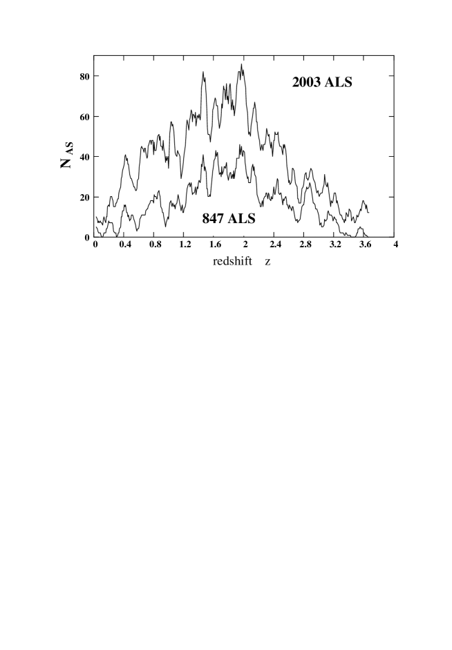
Figure 1: $z$-distributions of absorption-line systems observed in QSO spectra within the redshift interval $z=0.0$ – 3.7: (i) 847 systems are taken from the catalogue by Junkkarinen et al. (1991) and (ii) 2003 systems – from the catalogue by Ryabinkov et al. (2003) (see text).

Fig. 1 demonstrates two $z$-distributions $N_{\rm AS}(z)$ of ALSs containing absorption lines of heavy elements within the redshift interval $z=0.0$ – 3.7. One of them is obtained using 847 systems from the catalog by Junkkarinen et al. (1991) and the second one is based on 2003 systems registered in the spectra of 661 QSOs (emission redshifts within $z_{e}=$0.29 – 4.9) from the catalog by Ryabinkov et al. (2003). All ALSs under consideration comprise lines of heavy elements and may include up to 20 – 30 absorption lines detected in different regions of QSO spectra (predominantly within the interval 3000 – 8000 Å). We exclude ALSs consisting only of neutral hydrogen lines as well as damped Ly$\alpha$ absorption systems (DLA). All redshifts $z_{j}$ registered in spectra of each QSO and fallen into the velocity interval $\,\delta v=$500 km s^-1 are treated as a single absorption system with an averaged redshift $z_{a}=(\sum_{j=1}^{n_{a}}z_{j})/n_{a}$, where $n_{a}$ is a number of redshifts within the interval. Both distributions in Fig. 1 are obtained using so-called sliding-average approach which represents a set of consecutive displacements of the averaging bin $\Delta_{\rm z}=0.071$ along $z$-axis with a step $\delta_{\rm z}=0.01$.

A comparison of the two $z$-distributions (Fig. 1) reveals similar patterns of the peaks and dips relatively smooth curves. The positions of majority of the peaks and dips remain the same after the extension of statistics and some of them become more significant. There are only a few exceptions concerned with splitting of some initially single peaks into double ones and an appearance of new peaks (see Table 1).

In Papers I and II the statistical analysis of ALSs was performed using the averaging bin $\Delta_{\rm z}=0.071$. This value was chosen with employing the $\chi^{2}$-criterion as a measure of the most significant deviations of the $z$-distributions obtained for different values $\Delta_{\rm z}$ from the hypothesis of the uniform distribution (with use of the trend subtraction). On this way the results of statistical considerations could be sensitive to artificial non-uniformities induced by a separation of the whole sample of the redshifts into bins. To exclude sensitivity of our results to the effects of the averaging bins we employ in this paper predominantly out-of-bin statistical technique. In particular, in Section 2 we apply a continuous wavelet transform to the whole sample of ALS redshifts to study in details the peak-and-dips sequence.

In Section 3, we demonstrate isotropy of the $z$-distribution, i.e., approximate independence the peak/dip positions of observation directions. In Section 4, we focus on a presumable regularity (quasi-periodicity) of the $z$-distribution. In Section 5, we examine properties of the one-dimensional correlation function. In Section 6, a polemic on the presence of periodicities in the distribution of QSO redshifts is outlined and possible selection effects in our analysis are briefly discussed. Conclusions and a short discussion of possible interpretations of the results are considered in Section 7.

2 Wavelet transform and non-uniformity of the $z$-distribution

In this section, we use the wavelet transform for the analysis of the consecution of all redshifts under consideration within the interval $z=0.0$ – 3.7 without subdividing the $z$-points into certain statistical bins. The wavelet transform is a way to disclose a difference of the redshift distribution from a smooth dependence and to reveal a set of condensations and depressions (peaks and dips) beyond the Poisson fluctuations. Actually, the wavelet analysis is effective when a signal has no evident periodicity and contains different sets of wave number (frequency) components in different space (time) regions. This method appears to be appropriate for the study of the non-uniformities visible in Fig.  1 and allows us to estimate statistical significance of the peaks and dips in the $z$-distribution of ALSs. Detailed information on the wavelet analysis and its applications in physics and astrophysics may be found in numerous books, reviews, and papers (e.g., Chui 1992, Astaf’eva 1996, Dremin, Ivanov & Nechitai’lo 2001 and references therein).

We apply so called “Mexican hat” wavelet:

$$\psi_{K_{x}}(x,y)=A\left[1-u^{2}\right]\exp\left[-{u^{2}\over 2}\right];\,\,\,\,\,\,u\equiv u(x,y)=(x-y)K_{x},$$ (1)

where $x$ is the current one-dimensional coordinate, $y$ is the translation of the wavelet along the coordinate axis, $K_{x}$ is an analog of the wave number for one-dimensional Fourier transform, and $A=A(K_{x})$ is a normalizing function. Usually, the value $1/K_{x}$ is called a dilation or a scale parameter. The wavelet (1) is proportional to the second derivative of the Gaussian distribution $\exp[-u^{2}/2]/\sqrt{2\pi}$ taken with sign $(-)$. The zero-momentum of Eq. (1) $\int{\rm d}x\,\psi_{K_{x}}(x,y)=$ $\int{\rm d}y\,\psi_{K_{x}}(x,y)$ is equal to zero in accordance with the admissibility condition (e.g., Chui 1992).

Let we have a signal $F(x)$, where $F(x)\in{\large L}^{2}$-space of normalized functions determined over the real axis $x$. Then, the coefficients of the continuous wavelet transform are

$$S(K_{x},y)=\int{\rm d}x\,F(x)\psi_{K_{x}}(x,y),$$ (2)

where the integration is carried out over the real axis. We obtain two-dimensional scanning of the signal, the wave number $K_{x}$ and the coordinate $y$ being independent variables.

In this paper, we obtain the coefficients (2) in an unconventional manner when the signal $F(z)$ is treated as the consecution of the discrete redshifts $z_{i}\,$ ($i=1,2,...$) inside the considered interval (similar approach was suggested by Slezak et al. 1993). We approximately present $F(z)$ as the sum of normalized delta functions localizing positions $z_{i}$ of all points in the sample:

$$F(z)\approx\sum_{i=1}^{{\rm N}_{\rm tot}}{2\pi\over{\cal K}_{z}^{\rm m}}\,\delta(z-z_{i});\,\,\,\,\,\,\,\,\,\,\int_{-\infty}^{\infty}{\rm d}z\,|F(z)|^{2}\approx{2\pi\over{\cal K}_{z}^{\rm m}}\,{\rm N}_{\rm tot},$$ (3)

where ${\cal K}_{z}^{\rm m}\gg 2\pi$ is an upper boundary of all wave numbers $(K_{z}\leq{\cal K}_{z}^{\rm m})$ involved in the analysis, ${\rm N}_{\rm tot}$ - is a number of all absorption systems in the sample, in our case ${\rm N}_{\rm tot}=2003$.

Following Eqs. (2) and (3), the wavelet transform of the function $F(z)$ yields the sum over all redshifts:

$$S(K_{z},z)={2\pi\over{\cal K}_{z}^{\rm m}}\,\sum_{i=1}^{{\rm N}_{\rm tot}}\psi_{K_{z}}(z_{i},z)=A(K_{z})\,\sum_{i=1}^{{\rm N}_{\rm tot}}\left[1-u_{i}^{2}\right]\exp\left[-{u_{i}^{2}\over 2}\right],$$ (4)

where $u_{i}\equiv u(z_{i},\,z)=(z_{i}-z)K_{z}$, the variables $K_{x}$ and $y$ in Eq. (2) are replaced by $K_{z}$ and $z$, respectively; in the second equality of Eq. (4) the factor of $2\pi/{\cal K}_{z}^{\rm m}$ is included in the normalizing function $A(K_{z})$.

Under the assumption of the uniform distribution of points $z_{i}$ over the interval $z=0.0$ – 3.7 the value $S(K_{z},z)$ represents a random function obeying approximately to the Gaussian distribution (${\rm N}_{\rm tot}\gg 1$). The mean value of the distribution $\mu[S(K_{z},z)]$ is equal to zero:

$$\mu[S(K_{z},z)]={1\over Z_{\rm max}}\sum_{i=1}^{{\rm N}_{\rm tot}}\,\int_{0}^{Z_{\rm max}}{\rm d}z_{i}\,\psi_{K_{z}}(z_{i},\ z)=0,$$ (5)

where the upper limit is $Z_{\rm max}=3.7$ and the mean squared deviation $\sigma(S(K_{z},z))$ may be put equal to unity:

$$\sigma^{2}[S(K_{z},z)]={1\over Z_{\rm max}}\sum_{i=1}^{{\rm N}_{\rm tot}}\,\int_{0}^{Z_{\rm max}}{\rm d}z_{i}\,\psi_{K_{z}}^{2}(z_{i},\ z)=1.$$ (6)

The latter condition allows one to determine $A=A(K_{z})$ (in general case $A=A(K_{z},z)$). Using Eqs. (4), (6) and neglecting terms of the orders of $\exp(-K_{z}^{2}z^{2})\ll 1$ and $\exp[-K_{z}^{2}(Z_{\rm max}-z)^{2}]\ll 1$ one can approximately write

$$A(K_{z})\,\approx\,\sqrt{{4\,K_{z}\,Z_{\rm max}\over 3\,\sqrt{\pi}\,{\rm N}_{\rm tot}}}\,.$$ (7)

Such a normalization allows to measure naturally two-dimensional wavelet coefficients $S(K_{z},z)$ in units of the standard deviation.

To decontaminate the wavelet coefficients $S(K_{z},z)$ from noise (e.g., Romeo et al. 2003, 2004) at small scales (high $K_{z}$) and from the trend at large scales (low $K_{z}$) we exploit so-called spectral filtration. For this aim, one can calculate the energy spectrum of the wavelet transform

$$E_{S}(K_{z})\simeq\,\sum_{n}\,S^{2}(K_{z},z_{n}),$$ (8)

where index $n=1,2,...363$ runs over the chosen interval ($0.04\leq z\leq 3.67$) with a small step ($\delta_{z}=0.01$).

If we admit that the distribution of $S(K_{z},z)$ is Gaussian (with zero mean value and unit dispersion) and all $S(K_{z},z_{n})$ in Eq. (8) are statistically independent (see below), then the value $E_{S}(K_{z})$ obeys to the $\chi^{2}$–distribution with 363 degrees of freedom. In this case we can fix a certain tabulated value $\chi_{1-p}^{2}$ at a given significance level $p$ (e.g., $3\sigma$, $p=0.0025$) and select the region of $K_{z}\leq 28$, where $E_{S}(K_{z})$ exceeds this level (critical interval for the hypothesis of the random distribution of the redshifts). On the other hand, at $K_{z}\;\raise 1.29167pt\hbox{$<$\kern-7.5pt\raise-4.73611pt\hbox{$\sim$}}\;14$ the value $E_{S}(K_{z})$ displays a sharp rise caused by the smooth dependence (trend) of the $z$-distribution (see Fig. 1). As a result we choose a representative interval $15\leq K_{z}\leq 28$, which is consistent with significant variations of the z-distribution, and cancel $S(K_{z})$ for all others $K_{z}$.

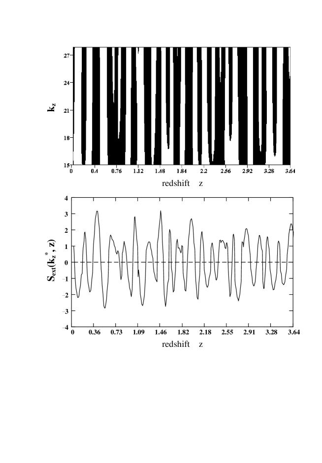
Figure 2: Results of the wavelet transformation. Upper panel: two-dimensional coefficients of the wavelet transform $S(K_{z},z)$; black strips illustrate positive values ($S>0$), white strips – negative values ($S<0$). Lower panel: extremal values of $S(K_{z},z)$ satisfying to the condition $|S_{\rm ext}(K_{z}^{*},z)|=$ max $(|S(K_{z},z)|)$, where $K_{z}$, and $K_{z}^{*}$ belong to the intervals $15\leq(K_{z},\ K_{z}^{*})\leq 28$.

The upper panel of Fig. 2 illustrates the two-dimensional wavelet coefficients $S(K_{z},z)$ in the chosen interval of $K_{z}$. One can see almost vertical alternating black and white strips corresponding to positive (enhanced) and negative (reduced) values of the wavelet coefficients, respectively. Centers of the strips do not change for different $K_{z}$ and these centers are consistent with the centers of peaks $z_{\rm max}$ and dips $z_{\rm min}$ obtained earlier in Papers I and II (see Table 1).

Table 1: Redshift values $z_{\rm max}$ (maxima) and $z_{\rm min}$ (minima) of the $z$-distribution of ALSs${}^{\leavevmode\nobreak\ a)}$.

299 C IV & 216 Mg II		847 ALSs					2003 ALSs
Paper I		Junkkarinen et al. (1991)					Ryabinkov et al. (2003)
$N_{\rm AS}(z)$ – bin statistics		$N_{\rm AS}(z)$ – bin statistics					Wavelet analysis
${\bf z_{\rm max}}$		${\bf z_{\rm min}}$	Significance	${\bf z_{\rm max}}$	Significance		${\bf z_{\rm min}}$	Significance	${\bf z_{\rm max}}$	Significance
			level		level			level		level
		0.10	2$\sigma$	0.22	2$\sigma$		0.11	2$\sigma$	0.22	2$\sigma$
0.44		0.31	3$\sigma$	0.45	3$\sigma$		0.30	2$\sigma$	0.42	3$\sigma$
							0.55	3$\sigma$	0.68	1.5$\sigma$
0.77		0.58	3$\sigma$	0.79	3$\sigma$		–		–
							0.81	1$\sigma$	0.87	1$\sigma$
1.04		0.96	2$\sigma$	1.10	1$\sigma$		0.97	2$\sigma$	1.05	3$\sigma$
1.30		1.18	1$\sigma$	1.28	1$\sigma$		1.16	2.5$\sigma$	1.28	1$\sigma$
1.46		1.35	1$\sigma$	1.44	2$\sigma$		1.38	1$\sigma$	1.46	3$\sigma$
1.63		1.54	2$\sigma$	1.63	2$\sigma$		1.55	2.5$\sigma$	1.62	2$\sigma$
1.78		1.71	1$\sigma$	1.75	1$\sigma$		1.68	2$\sigma$	1.77	1$\sigma$
1.98		1.84	1$\sigma$	1.96	2$\sigma$		1.87	2$\sigma$	1.97	2.5$\sigma$
2.14		2.07	1$\sigma$	2.13	1$\sigma$		2.07	2$\sigma$	2.15	2$\sigma$
–		2.24	2$\sigma$	–			2.23	1.5$\sigma$	2.31	1$\sigma$
2.45		–		2.42	3$\sigma$		2.38	1$\sigma$	2.49	1.5$\sigma$
2.64		–		–			2.61	2$\sigma$	2.66	1.5$\sigma$
2.86		2.72	3$\sigma$	2.87	3$\sigma$		2.74	2$\sigma$	2.87	2$\sigma$
							3.00	1.5$\sigma$	3.09	1.5$\sigma$
–		3.05	2$\sigma$	3.16	2$\sigma$		–		–
							3.16	1.5$\sigma$	3.22	1.5$\sigma$
–		3.40	3$\sigma$	–			3.32	1.5$\sigma$	3.41	1$\sigma$
–		–		3.56	2$\sigma$		3.49	1.5$\sigma$	3.61	2.5$\sigma$

^a) Bold values $z_{\rm max}$ mark divergences between our previous and present results

The lower panel of Fig. 2 illustrates how wavelet coefficients allow one to localize positions of the centers of the bands and estimate significance levels of the peaks and dips. The panel shows the z-dependence of the extremal wavelet coefficients $S_{\rm ext}(K_{z}^{*},z)\equiv S(K_{z}^{*},z)$, where the values $K_{z}^{*}=K_{z}^{*}(z)$ are obtained numerically for each fixed $z$ from the condition $|S_{\rm ext}(K_{z}^{*},z)|=$ max($|S(K_{z},z)|$). The extremal wavelet coefficients represent the variations of $S(K_{z},z)$ in the most pronounced form..

Positions of peaks $z_{\rm max}$ and dips $z_{\rm min}$ are determined as weighted mean values (centers of gravity) of the points $S_{\rm ext}(K_{z}^{*},z)$ forming the peaks or dips with respect to zero level. The accuracy of such determination is $\pm 0.02$. As it is seen from Table 1 majority of the values $z_{\rm max}$ and $z_{\rm min}$ calculated for the wavelet coefficients are close to the values $z_{\rm max}$ and $z_{\rm min}$ obtained in our previous statistical studies. There are only a few exceptions (indicated in Table 1 by bold font) concerned with two cases of splitting of peaks into double ones at $z_{\rm max}=0.79$ and 3.16, and three cases of appearance of new peaks at $z_{\rm max}=2.31$, 2.66 and 3.41. The latter peaks are located on the decreasing part of the $N_{\rm AS}(z)$ distribution (Fig. 1) where statistics is essentially poorer. Note that the peak at $z_{\rm max}=2.66\pm 0.02$ was obtained earlier by the statistical analysis of C IV doublets (first column in Table 1).

It follows from Table 1 that, in general, there is a good agreement between the new and previous results. In addition, the significance levels of the peaks and dips estimated using the wavelet coefficients $S_{\rm ext}(K_{z}^{*},z)$ are systematically higher than similar significance levels obtained in Papers I and II.

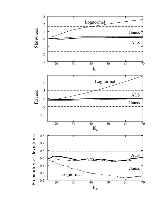
Figure 3: Statistical comparison of wavelet transformations produced for the $z$-distribution of ALSs (thick lines), the Gaussian distribution of 2000 random $z$-points with periodical variations of the mean value (thin lines – ‘Gauss’), the lognormal distribution simulated on the base of the same Gaussian model (thin lines – ‘Lognormal’; see text). Upper panel: skewness, middle panel: excess (kurtosis), lower panel: probability of $\pm$-deviations in a dependence on $K_{z}$ within the interval $15\leq K_{z}\leq 70$. Dashed lines indicate the boundaries of critical regions at the significance level $3\sigma$.

A set of our numerical simulations of the wavelet coefficients $S(K_{z},z)$ produced for Poisson distribution of $N_{\rm tot}$ points $z_{i}$ using Eqs. (4) and (7) has shown that the mean squared deviation $\sigma$, or the variance $\sigma^{2}$, calculated for the wavelet coefficients turned out to be lower than unity. Actually, the random wavelet coefficients obtained at different $z$ and $K_{z}$ are not independent. In particular, we have $\sigma^{2}[S(K_{z},z)]=0.56$ at $K_{z}=15$ and $\sigma^{2}[S(K_{z},z)]=0.66$ at $K_{z}=28$. Such a decrease of the variance results in an increase of the significance levels of $S(K_{z},z)$. Consequently, the significance levels of peaks and dips indicated in Table 1 may be regarded as minimal estimations. Additional calculations have shown that statistical dependence of $S(K_{z},z)$ at different $K_{z}$ and $z$ in Eq. (8) leads to lowering of the boundary $\chi_{1-p}^{2}$ and as a result to expansion of the critical interval of $K_{z}$ into the range of higher $K_{z}$. Thus the chosen interval $15\leq K_{z}\leq 28$ may be treated as minimal critical interval or minimal representative interval appropriate to the alternative hypothesis of a regular origin of the peaks and dips in Fig. 2.

In this section and hereafter we use the hypothesis of Gaussian distribution of the absorbing matter as basic one for estimations of the statistical significance of the peaks and dips and their regularity. It follows from the results discussed that the simple Gaussian model for the distribution of ALSs may be rejected on the significance level $\;\raise 1.29167pt\hbox{$>$\kern-7.5pt\raise-4.73611pt\hbox{$\sim$}}\;2\sigma$. However, it is worthwhile to verify consistency of the ALS distribution with a wider class of Gaussian-like and non-Gaussian distributions. For this aim, we simulated two particular stochastic models (basic hypotheses) of the absorbing matter distribution:
(i) Gaussian binned distribution of 2000 redshift points $z_{i}$ with a periodical expectation $\mu(z)$ and the variance equal to unity:

$$P\left[x(z)\right]={1\over\sqrt{2\pi}}\exp\left\{-\left[x(z)-\mu(z)\right]^{2}/2\right\},$$ (9)

where $x(z)=[n(z)-n_{0}]/\sqrt{n_{0}}$, $\ n(z)$ is a number of random points within a bin $z\pm\Delta_{\rm z}/2,\,$ $\Delta_{\rm z}=0.071$, $n_{0}$ is a mean number of points averaged over all bins; $\mu(z)=2.5\cos(2\pi z\ 16/Z_{\rm max})$, numbers 2.5 and 16 are chosen as an amplitude (significance level) and harmonic number of the variations; (ii) so-called lognormal random field suggested in literature as a plausible model for density fluctuations in the Universe (e.g., Coles & Jones 1991, Bi & Davidsen 1997). The lognormal distribution of the same number of points has been produced numerically from the distribution (9) by a transformation of the variable $x(z)$ into $y(z)=\exp[x(z)]$. Accordingly, the wavelet transforms $S(K_{z},z)$ have been calculated for both distributions using simple modification of Eq. (4) adjusted to binned statistics.

Fig. 3 displays a comparison of statistical symmetry properties of the wavelet transformations produced for two models (i) and (ii) with $S(K_{z},z)$ calculated for ALSs. Three panels in the Fig. 3 represent (from top to bottom) the skewness, kurtosis (excess), and probability of sign deviations (criterion of signs) calculated in standard technique. One can notice that the symmetry properties of the wavelet coefficients obtained for ALSs and ‘Gauss’ model are statistically close. For both samples the skewness and excess are situated near zero for all values $K_{z}$ and the probability of $\pm$ deviations variates near the number 0.5 corresponding to symmetrical distributions. On the other hand, the ‘Lognormal’ model notably differs from both symmetrical distributions by its asymmetry.

These results and results of our additional calculations carried out for the standard Gaussian field and its transformation into the lognormal random field confirm that the Gaussian (or Gaussian-like) distribution may be chosen as a background for the statistical analysis of ALS. Let us remind as well that in our consideration we treat all ALSs detected along each line of sight and fallen into the averaging velocity interval $\delta v$ (predominantly $\delta v=500$ km/s) as a single redshift. That smoothes away all nonlinear stochastic fluctuations of the $z$-distribution and approaches them to Gaussian-like random field.

3 Isotropy of the distributions

Let us test isotropy (or anisotropy) of the ALS distribution comparing the z-dependences of the wavelet coefficients $S_{\rm ext}(K_{z}^{*},z)$ calculated for different hemispheres. The procedure is similar to that used in Papers I and II for verification of a dependence of $N_{\rm AS}(z)$ (see Section 1) on orientations of hemispheres.

Figure 4: $z$-dependences of the wavelet coefficients $S_{\rm ext}(K_{z}^{*},z)$ (see text) calculated for 24 hemispheres in the equatorial (upper panel) and Galactic (lower panel) coordinate systems. Upper panel: the hemispheres are determined by the right ascensions $\alpha_{c}-90^{\circ}\leq\alpha\leq\alpha_{c}+90^{\circ}$, $\alpha_{c}$ stands for hemisphere centers, and declinations $-90^{\circ}\leq\delta\leq+90^{\circ}$; the vertical axis represents $\alpha_{c}$ in degrees plotted with the step $15^{\circ}$ ($1^{h}$). Lower panel: the hemispheres are determined by the Galactic longitudes $l_{c}-90^{\circ}\leq l\leq l_{c}+90^{\circ}$, $l_{c}$ stands for hemisphere centers, and latitudes $-90^{\circ}\leq b\leq+90^{\circ}$; the vertical axis represents $l_{c}$ in degrees plotted with the step $15^{\circ}$.

Fig. 4 shows two sets of redshift dependences of the value $S_{\rm ext}(K_{z}^{*},z)$ plotted for 24 hemispheres. Both panels in Fig. 4 may be treated as two-dimensional distributions of the wavelet coefficients $S_{\rm ext}$. The vertical axis on the upper panel (equatorial CS) represents the right ascension of the hemisphere centers $\alpha_{c}$ (in degrees), the horizontal axes corresponds to the redshifts $z$. The black strips display positive (enhanced) values of the wavelet coefficients, $S_{\rm ext}>0$, and the white strips display negative (reduced) values of the wavelet coefficients, $S_{\rm ext}<0$. One can see the set of continuous vertical black and white strips with centers at the same values of $z_{\rm max}$ and $z_{\rm min}$ as indicated in Table 1, i.e., $z_{\rm max}=$ 0.42, 1.05, 1.28, 1.46, 1.97, 2.87, 3.09 and $z_{\rm min}=$ 0.11, 0.30, 0.55, 0.97, 1.16, 1.38, 1.87, 2.23, 2.74, 3.00, 3.32. These values of $z_{\rm max}$ and $z_{\rm min}$ are independent of $\alpha_{c}$ within statistical errors. The rest black and white strips are more fragmentary. However, the strips comprise segments which are notably longer than $180^{\circ}$. Such segments exceed possible effects of enhanced concentration of ALSs (clumps) at certain $z$ in separate directions and can not be reproduced by overlapping of hemispheres.

The vertical axis on the lower panel represents the Galactic longitude of the hemisphere centers $l_{c}$ (in degrees). It is clear from comparison of the upper and lower panels that the positions of the vertical strips as well as their width do not change (within statistical uncertainties) if we use the Galactic coordinates instead of the equatorial ones. Consequently, the wavelet coefficients do not depend substantially on the orientation of hemispheres. We calculated the correlation coefficients for the $z$-distributions in 12 pairs of opposite (independent) hemispheres and found moderate positive correlation at the significance level $\;\raise 1.29167pt\hbox{$>$\kern-7.5pt\raise-4.73611pt\hbox{$\sim$}}\;2-3\sigma$, probably due to variations of peak-and-dip profiles with relatively stable centers of gravity.

On the other hand, our calculations of the wavelet coefficients within separate quadrants ($\alpha_{c}\pm 45^{\circ}$) instead of hemispheres ($\alpha_{c}\pm 90^{\circ}$) display more irregular black and white domains around certain $z_{\rm max}$ and $z_{\rm min}$. As a result the strips-like picture (as in Fig. 4) turns out to be more fragmentary.

Thus our wavelet analysis of the ALS redshifts gives evidence in favour of (i) the existence of the statistically significant ($\;\raise 1.29167pt\hbox{$>$\kern-7.5pt\raise-4.73611pt\hbox{$\sim$}}\;2\sigma$) peaks and dips in the z-distribution of the ALSs at certain $z_{\rm max}$ and $z_{\rm min}$ and (ii) approximate independence $z_{\rm max}$ and $z_{\rm min}$ obtained for different hemispheres of hemisphere orientations.

4 Regularity (quasi-periodicity) of the peaks and dips

The positions of the maxima $z_{\rm max}$ and minima $z_{\rm min}$ presented in Table 1 are distributed nonuniformly. For instance, it may be verified numerically that the power spectrum calculated for the whole sequence of redshift points (see below) displays no significant peaks in a wide region of $z$-scales ($z$-periods) including all intervals between neighbour maxima or minima in Table 1. Therefore, to reveal some regularity (e.g., quasi-periodicity) in the sequence of the peaks and dips we need to use so-called rescaling functions $\tau=f(z)$ which satisfy, e.g., to periodicity condition:

$$\tau_{\rm max}^{\rm m+1}-\tau_{\rm min}^{\rm m}=f(z_{\rm max}^{\rm m+1})-f(z_{\rm min}^{\rm m})={\rm const},$$ (10)

where $m=1,2,...$ – is the continuous numeration of the maxima and minima.

In Papers I and II we tested the quasi-periodicity of the ALS distribution using several simple rescaling (trial) functions of $z$ including the function $\log(1+z)$ which attracts special attention in literature in search of a periodicity of the QSO $z$-distribution (see Section 6). In contrast to these papers, our new calculations based on the extended statistical sample have not revealed a significant (at level $>2\sigma$) periodicity with respect to the same trial functions. Therefore, we perform the power-spectrum analysis using some special trial function (unless the different functions are discussed) which appears to be more appropriate for testing of the quasi-periodicity of the ALS distribution:

$$\tau_{i}=\tau(z_{i})=\sinh^{-1}[(\eta(z_{i})-a_{1})\,a_{2}],$$ (11)

where $i=1,2,...{\rm N}_{\rm tot}$ is a numeration of all ALSs (N${}_{\rm tot}=2003$); $a_{1}$ and $a_{2}$ are constants; $\eta(z)$ is the conformal time defined by

$$\eta(z_{i}) = \int_{0}^{z_{i}}{1\over\sqrt{\Omega_{\rm M}(1+z)^{3}+(1-\Omega_{\rm M}-\Omega_{\rm\Lambda})(1+z)^{2}+\Omega_{\rm\Lambda}}}\,\,{\rm d}z,$$

(12)

where we choose $\Omega_{\rm M}=0.3$ and $\Omega_{\rm\Lambda}=0.7$.

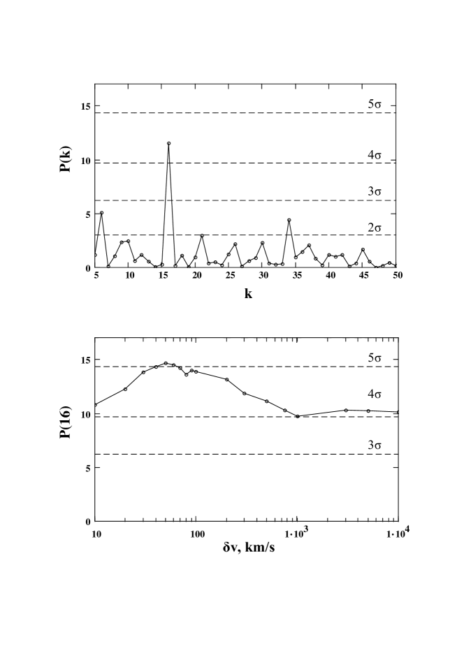
Figure 5: Power spectra P$(k)$, $k$ is the harmonic number, calculated with using the trial function (11),  (12) for the complete sample of the values $z_{i},\,i=1,2,...{\rm N}_{\rm tot}$ (see text). Upper panel represents P$(k)$ defined by Eq. (13) at the velocity interval $\delta v=500$km s^-1 of AS associations (along each line of sight) into single redshifts $z_{i}$ (see Section 1). The main peak corresponds to $k=16$. Lower panel plots the dependence of the highest-peak value P$(k=16)$ on the interval $\delta v$. The horizontal dash lines specify the confidence levels $\beta=0.95$ ($2\sigma$; only on the upper panel), $\beta=0.998\ (3\sigma)$, $\beta=0.999936\ (4\sigma)$, $\beta=0.9999994\ (5\sigma)$, respectively.

The spectral power of the distribution is calculated without the use of statistical bins $\Delta_{\rm z}$ (e.g., Karlsson 1977, Arp et al. 1990, Paper I):

$${\rm P}(k)={1\over{\rm N}_{\rm tot}}\left\{\left[\sum_{i=1}^{{\rm N}_{\rm tot}}\cos\left({2\pi k\tau_{i}\over\hat{\tau}}\right)\right]^{2}\,+\,\left[\sum_{i=1}^{{\rm N}_{\rm tot}}\sin\left({2\pi k\tau_{i}\over\hat{\tau}}\right)\right]^{2}\right\},$$ (13)

where $\tau_{i}$ is given by Eq. (11), $\hat{\tau}$ $=\tau(z_{{\rm N}_{\rm tot}})-\tau(z_{1})$ is the whole interval of values $\tau_{i}$, and $k$ is a harmonic number. The periodicity yields the peak in the power spectrum ${\cal P}={\rm max}$ (P$(k)$) with a confidence probability

$$\beta=[1-\exp(-{\cal P})],$$ (14)

where the confidence level is defined with respect to the hypothesis of the uniform distribution of the values $\tau_{i}$.

Results of the power-spectrum analysis are sensitive to the averaging velocity interval $\delta v$ of the ALS associations into separate redshifts (see Sect. 1). The upper panel of Fig. 5 plots the results of the calculations based on Eq. (13), where $\delta v$=500 km s^-1 and the constants in Eq. (11) are $a_{1}$=1.26, $a_{2}$=3.37. One can see that in the represented interval of $k$ the only appreciable peak P$(k)$ appears for $k=16$ at the significance level $>4\sigma$. This peak corresponds to a periodicity in units of the function (11) with the period $\Delta\tau=\hat{\tau}/k=0.199\pm 0.001$. Note that the most significant peak is very sensitive to variations of the values $a_{1}$ and $a_{2}$ at fixed $\Omega_{\rm M}$ and $\Omega_{\rm\Lambda}$ (or variations of $\Omega_{\rm M}$ and $\Omega_{\rm\Lambda}$ at fixed $a_{1}$ and $a_{2}$). The deviations of $a_{1}$ and $a_{2}$ from indicated values exceeding $\pm 0.01$ and $\pm 0.28$, respectively, reduce the peak P$(k)$ to the significance level $\;\raise 1.29167pt\hbox{$<$\kern-7.5pt\raise-4.73611pt\hbox{$\sim$}}\;3\sigma$.

The lower panel of Fig. 5 shows the dependence of the main peak amplitude P$(k=16)$ on the velocity interval $\delta v$. It is seen that the maximum of P$(k=16)$ increases smoothly with decreasing of $\delta v$ and reaches the significance level $>5\sigma$ at $\delta v=$50–70 km s^-1, being basically robust to variations of $\delta v$. Let us note that such an averaging of redshifts along each line of sight (up to $\delta v=10,000$ km/s) smoothes down possible effects of longitudinal clumping of absorbing matter.

In addition Fig. 6 demonstrates effects of plausible clumping of ALSs in fields perpendicular to lines of sight. We calculate the same power-spectrum as in Fig. 5 but with elimination of all groups of QSO spectra if their coordinates turn out to locate within any $1\times 1$ deg² square region on the celestial sphere. Similar significant peak $P(k)$ at $k=16$ as in Fig. 5 indicates weakness of transversal clumping effects in our analysis.

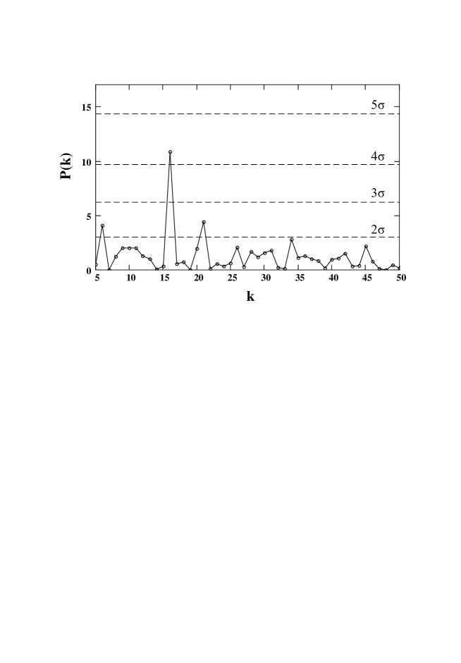
Figure 6: Same as in upper panel of Fig. 5 but for 1778 ALSs sampled with elimination of all groups of QSOs with their ALSs located within $1\times 1$ deg² square regions on the sky.

The rescaling function given by Eqs.  (11) and (12) is not unique. For example, following Alam et al. (2004) we may choose a model independent ansatz for the Hubble parameter

$$H(z) = H_{0}\,\sqrt{\Omega_{{\rm M}0}\,(1+z)^{3}+A_{0}+A_{1}(1+z)+A_{2}\,(1+z)^{2}};$$

$$\Omega_{{\rm M}0} = 8\pi G\ \rho_{0}/(3H_{0}^{2}),$$ (15)

where $H_{0}$ and $\rho_{0}$ are the Hubble constant and matter density at the present epoch ($z=0$). We calculate $P(k)$ replacing $\tau_{i}$ and $\hat{\tau}$ in Eq. (13) by the conformal time $\eta_{i}$ and $\hat{\eta}$ $=\eta(z_{{\rm N}_{\rm tot}})-\eta(z_{1})$, where the rescaling function $\eta(z)$ is given by Eq. (12) with the denominator replaced by $H(z)/H_{0}$ from (15). Varying $\Omega_{{\rm M}0}$ and the coefficients $A_{0},A_{1}$, $A_{2}$, and keeping the equality $A_{0}+A_{1}+A_{2}=1-\Omega_{{\rm M}0}$, we also obtain the significant peak $P(k)$ of the power spectra at $\Omega_{{\rm M}0}=0.3$ and $A_{0}=-0.61,A_{1}=3.11,A_{2}=-1.8$ on the level $\;\raise 1.29167pt\hbox{$>$\kern-7.5pt\raise-4.73611pt\hbox{$\sim$}}\;4\sigma$ (slightly lower than that in Fig. 5).

The other example of a rescaling function is the mean comoving number density of absorbers associated with filaments (the elements of so-called large scale structure; see Sect. 7) introduced by Demiański, Doroshkevich & Turchaninov (2000) in their Eqs.  (2.2) and (2.15) with the function $B(z)$ given by their Eq. (2.3a). Employing this rescaling function we obtain the peak of $P(k)$ at the same $k=16$ but even more significant ($>5\sigma$) than the peak in Fig. 5. However, additional powerful peaks of $P(k)$ (less significant than the main peak) also appear for this trial function. In this case the periodicity becomes more complex and requires a special consideration.

For comparison, using Eqs.  (13), (11) and (12) we have calculated additionally the power-spectrum $P(k)$ of the distribution of emission-line redshifts $z_{e}$ detected in the spectra of 661 original QSOs within the interval $z=0.29$–4.9. We have not revealed significant peaks (with significance $\;\raise 1.29167pt\hbox{$>$\kern-7.5pt\raise-4.73611pt\hbox{$\sim$}}\;3\sigma$) for a wide region of periods around $\Delta\tau\sim 0.2$. Thus we conclude that there is no straightforward coupling between possible periodicities of the $z$-distributions of ALSs and original QSOs. Note, however, that the sample of QSOs is not statistically representative.

To sum up the results of this section, we conclude that the appearance of significant peaks in the power spectra (calculated with different trial functions) may be regarded as additional evidence for reality of the peak-depression sequence in the $z$-distribution of ALSs and its nonrandom origin. At the same time this quasi-periodical distribution does not correlate with the distribution of the original QSOs.

5 One-dimensional correlation function

We determine a two-point correlation function $\xi(\delta\tau)$ for the sample of ALSs in an unconventional way. Specifically, the variable $\delta\tau$ substitutes a comoving distance $r$ between pairs of objects (e.g., galaxies or clusters of galaxies) in the standard two-point correlation function $\xi(r)$ (e.g., Peebles 1993, Landy & Szalay 1993, Kerscher, Szapudi & Szalay 2000, Jones et al. 2004, and references therein). In our consideration $\delta\tau$ is a measure of the separation of two arbitrary ALSs numerated by $i$ and $j$ ($i,j=1,2,...{\rm N}_{\rm tot}$, $i\neq j$) in units of the trial function $\delta\tau_{i,j}=|\tau_{i}-\tau_{j}|$ introduced by Eq.  (11). Accordingly, the intervals of the conformal time given by (12) and the redshifts are $\delta\eta_{i,j}=|\eta_{i}-\eta_{j}|$ and $\delta z_{i,j}=|z_{i}-z_{j}|$, respectively. Thus we can write:

$$\xi(\delta\tau)={{\cal N}_{\rm obs}(\delta\tau)\over{\cal N}_{\rm sim}(\delta\tau)}-1,$$ (16)

${\cal N}_{\rm obs}(\delta\tau)$ is the number of observed pairs of ALSs separated by the variables $\delta\tau_{i,j}$ within the range $\delta\tau\pm\Delta_{\tau}/2$, where $\Delta_{\tau}=0.07$ is the chosen bin width. ${\cal N}_{\rm sim}(\delta\tau)$ is the calculated number of cross pairs between the real sample of ASs and the points of a random sample simulated for the same intervals of $z$ or $\tau(z)$ and the same smoothed function (trend) as the real sample (e.g., Mo, Jing & Börner 1992). The both samples (real and simulated ones) have the same number of redshift points.

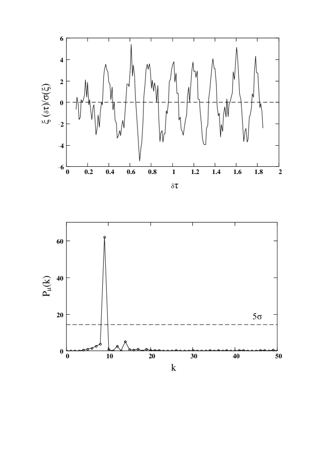
Figure 7: Upper panel: one-dimensional correlation function $\xi(\delta\tau)/\sigma(\xi)$ (see text) versus the interval $\delta\tau$ ($0.1\;\raise 1.29167pt\hbox{$<$\kern-7.5pt\raise-4.73611pt\hbox{$\sim$}}\;\delta\tau\;\raise 1.29167pt\hbox{$<$\kern-7.5pt\raise-4.73611pt\hbox{$\sim$}}\;1.9$) between the components of pairs of ALS redshifts (sampled at $\delta v=500$km s^-1); $\tau(z)$ is the trial function given by Eq. (11). Lower panel: power spectrum P${}_{\mu}(k)$ calculated for $\mu=\mu(\tau)=\xi(\delta\tau)/\sigma(\xi)$ according to Eq. (19); $k$ is the harmonic number.

Note that the variable $\delta\tau$ in Eq. (16) may be considered as a measure of the temporal separation of any two epochs in units of the scaling function (11). Actually, in our case the temporal interpretation of $\xi(\delta\tau)$ is more appropriate than the spatial one. Unlike the standard approach to the spatial two-point correlation functions (see below) the function (16) is based on the conception of a single reference center $\tau=0$ ($z=0$) concerned with the observer. Accordingly, all sampled points (redshifts) $\tau_{i}(z_{i})$ are distributed over concentric spherical layers (bins) independently of the directions to their original QSOs. We count up all redshifts $\tau_{j}$ inside a concentric layer ($\tau\pm\Delta_{\tau}/2$) with respect to any chosen point $\tau_{i}$ (out of this layer). All redshifts within a layer are treated as equivalent despite of various spatial (comoving) distances between them.

On the other hand, the function (16) differs from the correlation functions calculated by counting only line-of-sight pairs of the objects with different mutual comoving distances (e.g., Quashnock, Vanden Berk & York 1996, Broadhurst & Jaffe 2000), although, the results of both approaches may turn out to be quite consistent.

The upper panel of Fig. 7 displays the one-dimensional (two-point) correlation function (16) in units of the appropriate Poisson error $\sigma(\xi)$ calculated as follows (e.g., Peacock & Nicholson 1991):

$${\xi(\delta\tau)\over\sigma(\xi)}\approx{{\cal N}_{\rm obs}(\delta\tau)-{\cal N}_{\rm sim}(\delta\tau)\over\sqrt{{\cal N}_{\rm sim}(\delta\tau)}},$$ (17)

where

$$\sigma(\xi)={1+\xi\over\sqrt{{\cal N}_{\rm sim}(\delta\tau)}}.$$ (18)

One can see the sequence of positive and negative peaks with the significance $\;\raise 1.29167pt\hbox{$>$\kern-7.5pt\raise-4.73611pt\hbox{$\sim$}}\;4\sigma$ with respect to zero level. Let us notice presence of the long range ordering in dependence of $\xi(\delta\tau)/\sigma(\xi)$ on $\delta\tau$. We regard it as a consequence of the peak-and-dip structure in the z-distribution of ALSs (see Sect. 2).

The lower panel in Fig. 7 represents the result of the power spectrum analysis performed for the value $\mu=\mu(\delta\tau)=\xi(\delta\tau)/\sigma(\xi)$ according to the equation:

$${\rm P}_{\mu}(k)={1\over N_{\mu}D}\left\{\left[\sum_{m=1}^{N_{\mu}}f_{m}\cos\left({2\pi k\,\delta\tau_{m}\over\delta\hat{\tau}}\right)\right]^{2}\,+\,\left[\sum_{m=1}^{N_{\mu}}f_{m}\sin\left({2\pi k\,\delta\tau_{m}\over\delta\hat{\tau}}\right)\right]^{2}\right\},$$ (19)

where $f_{m}=\mu_{m}-<\mu>,\,\,$ $\mu_{m}=\mu(\delta\tau_{m}),\,\,$ $<\mu>\ =N_{\mu}^{-1}\,\sum_{m}^{N_{\mu}}\mu_{m}\,\,$ is the mean value of $\mu$, $D=\ <\mu^{2}>-<\mu>^{2}\,$ is the variance of $\mu$, and $<\mu^{2}>\ =N_{\mu}^{-1}\,\sum_{m}^{N_{\mu}}\ \mu_{m}^{2}\,$ is the mean squared value of $\mu$; the values $\delta\tau_{m}$ run over a set of points $m=1,2,...N_{\mu}$ of the variable $\delta\tau$ from 0.1 to 1.86 with the step 0.01. Thus $N_{\mu}=176$ is the full number of the points and $\delta\hat{\tau}=1.76$ is the whole interval of $\delta\tau_{m}$ variations under consideration. Note the strong single peak of P${}_{\mu}(k)$ at $k\simeq 9$ on the significance level well exceeding $5\sigma$. This peak manifests the periodicity of the correlation function with the period $\Delta\tau=0.199\pm 0.001$, which is in a good agreement with the periodicity found in Sect. 4.

The one-dimensional correlation functions $\xi(\delta\tau)$ and appropriate power spectra (19) were calculated also for ALS samples with different values of $\delta v$ and $\Delta v$, where $\delta v$ is the averaging velocity interval of ALS associations into single redshifts (see Sects. 1 and 4) and $\Delta v$ is the minimal velocity shift (along each line of sight) adopted for the sample of ALSs relative to the original QSO emission redshifts ($z_{e}$). In that way we exclude all ALSs with $z_{a}$ within the region associated with their own QSOs, i.e., at $z_{e}\geq z_{a}\geq z_{e}-\Delta v\,(1+z_{e})/c$. The values $\delta v$ and $\Delta v$ were changed within the intervals 10 – 10,000 km/s and 0 – 10,000 km/s, respectively. The results obtained are similar to that presented in Fig. 7. Thus the results are quite robust to the variations of ALS samples.

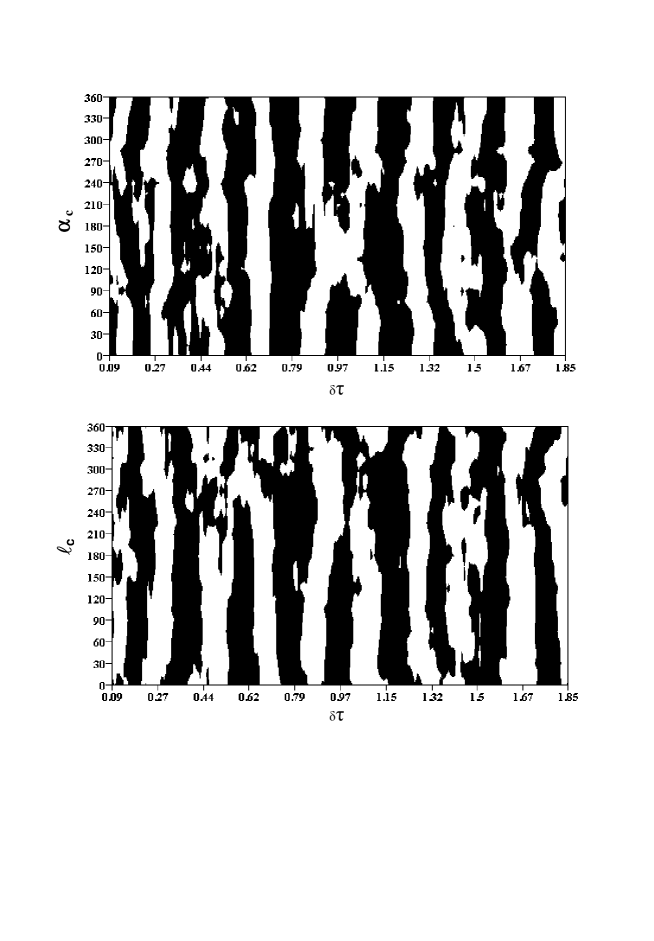
Figure 8: The correlation function $\xi(\delta\tau)$ of absorption systems calculated in 24 hemispheres for the equatorial (upper panel) and Galactic (lower panel) coordinate systems, respectively; $\xi>0$ – black strips and $\xi<0$ – white strips. Upper panel: the vertical axis indicates the right ascension of the hemisphere centers $\alpha_{c}$ (in degrees). Lower panel: the vertical axis indicates the Galactic longitudes of the hemisphere centers $l_{c}$ (in degrees). The horizontal axes show the interval of $\delta\tau$ between the components of ALS pairs.

For comparison, we have performed additional calculations of the standard two-point correlation function $\xi(r)$ (e.g., Landy & Szalay 1993, Jones et al. 2004), where $r$ is the comoving distance between the components of ALS pairs. The values $r$ were calculated using the formulae by Roukema (2001) with equatorial coordinates $\alpha_{i}$, and $\delta_{i}$ appropriate to ALSs (Section 3). For convenience, we employed the Hubble parameter $H(z)$ given by Eq. (15) with $\Omega_{{\rm M}0}=0.3$ and the same coefficients $A_{0},\ A_{1}$ and $A_{2}$ as indicated in Section 4. Let us remind that the rescaling function (12) with the model dependence $H(z)$ displays the significant periodicity of the ALS redshifts (see Section 4). We tested a periodicity of the function $\xi(r)$ (in a similar way as for $\xi(\delta\tau)$) using an analogue of Eq. (19) with the variable $\delta\eta=H_{0}r/c$ instead of $\delta\tau$. As a result, we have not revealed any significant peaks of P${}_{\mu}(k)$ and, consequently, significant periodicities of the spatial correlation function $\xi(r)$.

Fig. 8 shows two sets of the values $\xi(\delta\tau)/\sigma(\xi)$ as a function of $\delta\tau$ calculated for 24 hemispheres, i.e., the step of consecutive rotations is also $15^{\circ}$. Similar to Fig. 4 the upper and lower panels of Fig. 8 may be treated as two-dimensional distributions in the equatorial and Galactic coordinate systems, respectively. The black strips display the positive values of the correlation function ($\xi(\delta\tau)/\sigma(\xi)>0$) while the white strips display the negative ones. One can see again (cf. Fig. 4) that there is the set of continuous vertical black and white strips with centers at the same values $\delta\tau$ as on the upper panel of Fig. 7. It follows from comparison of the upper and lower panels that the positions of the vertical strips as well as their widths do not change essentially with transition from the equatorial to the Galactic coordinates, i.e., with changing of the axis of hemisphere rotations. Consequently, the two-point correlation function (similar to the wavelet coefficients in Sect. 3) is weakly sensitive to orientations of the hemisphere.

6 Distribution of Quasars and selection effects

The first peak at $z=1.95$ in the $z$-distribution of emission and absorption line redshifts in QSO spectra was found by Burbidge & Burbidge (1967). Then the quasi-periodical sequences of peaks and dips in the $z$-distribution of quasar emission lines were marked by many authors (e.g., Burbidge 1968, Cowan 1969, Karlsson 1971, 1977, 1990, Fang et al. 1982, Arp et al. 1990). Furthermore, several maxima and minima were detected in the distribution of absorption systems (e.g., Chu & Zhu 1989, Arp et al. 1990). Since the very beginning debates on availability of the periodicities in the redshift distribution of QSOs or QSO–galaxy pairs have been opened in the literature. There are many adherents of the statement that some type of the periodicity does really exist (e.g., Karlsson 1990, Khodyachikh 1990, Arp et al. 1990, Arp, Fulton & Roscoe 2005, Burbidge & Napier 2001, Napier & Burbidge 2003, Burbidge 2003, Bell 2004, and references therein) and their opponents (e.g., Box & Roeder 1984, Basu 1985, 2005, Scott 1991, Hawkins, Maddox & Merrifield 2002, Tang & Zhang 2005), who argue that the periodicity and the very set of peaks and dips in the QSO distribution are results of various selection effects.

At least a part of the authors standing for reality of the periodicity under discussion regards that as evidence for the hypothesis that QSOs (or essential part of them) represent some objects ejected from the nuclei of nearby active galaxies (e.g., Arp et al. 1990, 2005, Burbidge & Napier 2001, Bell 2004, and references therein). The redshifts of QSOs being larger than the redshifts of their parent galaxies have been assumed to have a non-cosmological “intrinsic” origin and display a set of preferred (discrete) quasi-periodical values. To our knowledge, there are two models discussed in literature which suggest different periodical sets of preferred redshifts. The first model has been applied mainly to QSOs and marginally to ALSs in QSO spectra (see above). That is described by so called Karlsson formula for the redshift periodicity $\Delta\log(1+z_{e})=0.089$ (e.g., Karlsson 1971, 1977, 1990, Arp et al. 1990, 2005, Burbidge & Napier 2001, Napier & Burbidge 2003). The second one was proposed by Bell (e.g., Bell 2002, 2004) for the “intrinsic” redshifts of QSOs and extended on a set of preferred redshifts of galaxies by Bell & Comeau (2003). According to both scenarios, the formation of ALSs on the lines of sight to the QSOs should have also occurred in the local vicinity of the Universe.

To test a possible correlation of the ALS distribution with expectations of the first model we have calculated the power spectrum of the sample of ALSs with respect to the trial function $\log(1+z)$. We have found no significant power peaks which would have a chance to be related with the period 0.089 or with a multiple value of it. According to the second QSO ejection model, appearance of the preferable $z_{\rm max}$ and $z_{\rm min}$ in the ALS distribution could be, in principle, interpreted as effects of an additional set of discrete “intrinsic” redshifts referred to galaxies. To test this statement one can compare the values of $z_{\rm max}$ from the last but one column in Table 1 with the set of intrinsic redshift components $z_{iG}[N,\ m]$ (where $N$ and $m$ are some quantum numbers) defined for galaxies by Eq. (B1) of Bell & Comeau (2003). Such a comparison shows that the set of the peaks $z_{\rm max}$ given in Table 1 are not consistent with the intrinsic redshifts of galaxies. Only three values $z_{\rm max}$ turn out to be equal (within the uncertainty $\pm 0.02$) to the values $z_{iG}$ from the set of 30 numbers at $N\leq 8$ within the interval $0.1\leq z\leq 3.7$. Thus we have found no traces of consistency between our results and the hypotheses of non-cosmological “intrinsic” redshifts of QSOs. Accordingly, in contrast with the papers quoted above , we assume that the redshift of the absorption lines $z_{a}$ is cosmological and the observed ALSs are associated with ionized gas in intervening galaxies or clusters of galaxies at cosmological distances along lines of sight to original QSOs.

The results of this paper may be biased by selection effects appropriate to the sample of ALSs. Taking it into account we undertook some special efforts in Paper I to minimize such effects in the statistical analysis. As it is shown in Table 1 the results obtained in Paper I are consistent with the results of the present paper. In Section 5 we discuss the effects of excluded regions of $z$ (within $\Delta v$) near QSO emission redshifts. Such exclusions allow us to avoid at least a part of selection effects related to so called associated regions of QSOs (e.g., Quashnock et al. 1996).

Furthermore, we failed to find similar periodicity (at significance level $\;\raise 1.29167pt\hbox{$>$\kern-7.5pt\raise-4.73611pt\hbox{$\sim$}}\;3\sigma$) in the $z$-distribution of the 661 original QSOs as it is revealed in the distribution of ALSs registered in their spectra (see Section 4). It separates possible selection effects biasing the statistics of QSOs (e.g., Box & Roeder 1984, Basu 2005, Tang & Zhang 2005) and those peculiar to the sample of ALSs involved in the analysis. It is worthwhile to note that the characteristic scale of redshifts $z$ which we consider in this paper ($\sim 0.18$) is essentially smaller than the scale ($\sim 0.48$) discussed for QSOs and QSO–galaxy pairs (e.g., Burbidge & Napier 2001) or the $z$-period ($\sim 0.62$) found for a sample of QSOs by Bell (2004). In particular, the narrowness of the peaks and dips obtained here makes the analysis of Basu (1979, 1983) less relevant to our results.

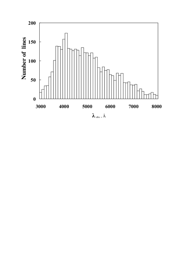
Figure 9: $\lambda$-distribution (spectroscopic completeness) of resonance doublets and single absorption lines of 15 ions which contribute mostly in the distribution of ALSs at different $z$; bin size of the histogram is $\Delta\lambda=100\AA$.

In Fig. 9 we test at least a part of possible selection effects concerned with a priori different probability to register absorption lines in QSOs spectra at different values of wavelength $\lambda$ within the observational interval (3000 – 8000 $\AA$). We choose 15 single lines or resonance doublets of the ions (C II, C IV, Mg I, Mg II, Si II, Si III, Si IV, N V, Al II, Al III, Fe II) most representative in the sample of ALSs under consideration and determine a number of wavelengths $\lambda=\lambda_{0}(1+z_{a})$ observed for each of them, where $\lambda_{0}$ is a laboratory value. Fig. 9 represents a histogram of the absorption lines as a result of count of the lines within bins $\Delta\lambda=100\AA$. One can see quite smooth histogram (so-called spectroscopic completeness) with two appreciable peaks between $4000$ – $4200\ \AA$ and $6300$ – $6600\ \AA$ (at significance level $\;\raise 1.29167pt\hbox{$>$\kern-7.5pt\raise-4.73611pt\hbox{$\sim$}}\;2\sigma$). These peaks are obviously not enough to explain all set of peaks in Fig. 1 as pure selection effects, i.e., as a consequence of peaks in the spectroscopic completeness. Although this conclusion does not completely exclude other selection effects in our statistical consideration.

7 Conclusions and discussion

The main results of the statistical analysis of 2003 absorption-line systems (ALSs) in the redshift range $z=0.0-3.7$ can be summarized as follows:

(1) The z-distribution of ALSs displays the statistically significant pattern of alternating maxima (peaks) and minima (dips) relative to a smooth curve. The positions of the maxima and minima (centroids of the peaks and dips) in the $z$-distribution are given in Table 1 with an accuracy $\pm 0.02$. These positions are predominantly not sensitive (within statistical uncertainties) to orientations of the hemispheres under statistical consideration. However, the correlation coefficients between the $z$-distributions calculated for 12 pairs of opposite (independent) hemispheres turn out to be moderately significant ($\;\raise 1.29167pt\hbox{$>$\kern-7.5pt\raise-4.73611pt\hbox{$\sim$}}\;2-3\sigma$) as a consequence of variations of the peak-and-dip profiles at relatively stable weighted centers of the peaks and dips.

(2) The sequence of peaks and dips reveals a certain regularity. The power spectrum calculated according to Eq. (13) with the rescaling function $\tau(z)$ given by Eqs. (11) and (12) displays the peak for the harmonic number $k=16$ (period $\Delta\tau=0.199\pm 0.001$) at the significance level exceeding $4\sigma$ (relatively to the hypothesis of the uniform distribution of ALSs over $\tau(z)$). The rescaling function $\tau(z)$ may be treated as a measure of temporal separations of the epochs with different $z$. Still more prominent peak at the same period $\Delta\tau$ arises in the power spectrum calculated for the two-point correlation function $\xi(\delta\tau)$ with the use of Eqs. (16) and (19).

(3) The obtained distribution of ALSs is likely to be coupled with the appearance of alternating pronounced (peaks) and depressed (dips) epochs in the course of the cosmological evolution, i.e., with the existence of some (relatively weak) spatial-temporal wave process. According to the cosmological principle (e.g, Peebles 1993) similar wave-like process would be observed from any spatial-temporal points in the Universe.

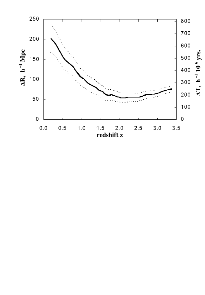
Figure 10: Comoving distance intervals $\Delta R$ (left vertical axis) and appropriate time intervals $\Delta T$ (right vertical axis) between successive neighbour peaks in the $z$-distribution of ALSs calculated as the intervals $\Delta\eta$ multiplied by $c/H_{0}$ and $1/H_{0}$, respectively (see text), and referred to appropriate redshifts $z$. The dotted lines illustrate $\pm\sigma$ deviations.

(4) Fig. 10 demonstrates the intervals of the comoving distance, $\Delta R=c\Delta\eta/H_{0}$, and the appropriate time, $\Delta T=\Delta\eta/H_{0}$, between neighbour peaks in dependence on the current redshifts $z$, where $\eta(z)$ is given by Eq. (12), $\Delta\eta$ runs over all successive intervals $\eta(z_{\rm max}^{l+1})-\eta(z_{\rm max}^{l})$, $\,l=1,2,...$ – numerates the peaks in the $z$-distribution of the ALSs (from top to bottom in Table 1). It follows from Fig. 10 that the characteristic scales of $\Delta R$ and $\Delta T$ vary in the ranges $\Delta R=(50$ – $200)\,h^{-1}$ Mpc and $\Delta T=(150$ – $650)\,h^{-1}$ Myr, respectively, where $h=H_{0}/100$ km(s Mpc)^-1.

Let us note that our treatment of the results obtained does not contradict to the existence of the Large Scale Structure (LSS) of the matter distribution in the Universe (e.g., Shandarin & Zeldovich 1989, Einasto et al. 2002, Tago et al. 2002, Demiański & Doroshkevich 2004, Jones et al. 2004, Eisenstein et al. 2005 and references therein). The spatial-temporal variations discussed here may be superimposed upon the process of formation and evolution of the LSS elements. It was noted in Sect. 3 that the strip-like picture represented in Fig. 4 becomes more fragmentary if the $z$-distributions are calculated for the quadrants ($\alpha_{c}\pm 45^{\circ}$) instead of the hemispheres. One can assume that more fragmentary patterns obtained for smaller sectors of observations appear not only as a result of a reduction of ALS statistics but also due to an interplay between LSS and the variations discussed here. In any case the possibility of such an interplay deserves a special investigation.

Extended discussions of the effects of the periodicity in the redshift distribution of galaxies on a scale about $130\leavevmode\nobreak\ h^{-1}$ Mpc was initiated in literature by the results of a pencil-beam survey of Broadhurst et al. (1990). These results also admit both interpretations either as a pure spatial quasi-periodic pattern of LSS constituents (set of clumps or walls and voids; e.g., Kaiser & Peacock 1991, van de Weygaert 1991, Dekel et al. 1992, Yoshida et al. 2001 and references therein) or as a temporal sequence of pronounced and depressed epochs becoming apparent in the matter distribution. The latter treatment is closer to our interpretation of the results represented here. However, our statistical approach does principally differ from the pencil-beam consideration.

The appearance of alternate pronounced and depressed epochs may be associated with intrinsic quasi-periodical properties of galaxies and/or their clusters (e.g., Liu & Hu 1998). On the other hand, it can be explained as an apparent pattern of density variations in terms of the cosmological scenarios considering scalar (scalar-tensor) fields and/or phase transitions at different evolutionary stages. Such effects may lead to temporal oscillations of the Hubble parameter $H(z)$ (e.g., Morikawa 1990, 1991, Hill, Steinhardt & Turner 1990, Perivolaropoulos & Sourdis 2002) and/or effective gravitational constant $G$ (e.g., Sisterna & Vucetich 1994, Busarello et al. 1994, González et al. 2001, Banerjee, Pavón & Sen 2003, Davidson 2005), peculiar velocity field (Hill et al., 1991), cosmological constant $\Lambda$ (e.g., Damour & Polyakov 1994, Dodelson, Kaplinghat, Stewart 2000), and, as a consequence, to apparent oscillations of the matter distribution with the redshift.

The rapid development of ground-based and space-born observational facilities in the optical, infrared, and near-ultraviolet ranges in recent years gives confidence that the hypothesis of the existence of the alternate epochs with enhanced and reduced concentrations of absorbing (or luminous) matter in the Universe may be tested in the nearest future.

Acknowledgments We are grateful to V.S. Beskin for suggestion to apply the wavelet analysis. We are also grateful both anonymous referees for useful critical remarks. The work has been supported partly by the RFBR (grant No.  05-02-17065a), and by the Federal Agency for Science and Innovations (grant NSh 9879.2006.2).

References

- Alam et al. (2004) Alam U., Sahni V., Saini T. D., Starobinsky A. A., 2004, MNRAS, 354, 275
- Arp et al. (1990) Arp H., Bi H.G., Chu Y., Zhu X., 1990, A&A, 239, 33
- Arp et al. (2005) Arp H., Fulton C., Roscoe D., 2005, preprint (astro-ph/0501090)
- Astaf’eva (1996) Astaf’eva N. M., 1996, Physics-Uspekhi, 39, 1085
- Banerjee et al. (2003) Banerjee N., Pavón D., Sen S., 2003, Gen. Relative. Grav., 35, 851
- Basu (1979) Basu D., 1979, A&A, 77, 255
- Basu (1983) Basu D., 1983, Astrophys. Sp. Sci., 92, 425
- Basu (1985) Basu D., 1985, A&A, 152, 63
- Basu (2005) Basu D., 2005, ApJ, 618, L71
- Bell (2002) Bell M.B., 2002, preprint (astro-ph/0211091)
- Bell (2004) Bell M.B., 2004, ApJ, 616, 738
- Bell & Comeau (2003) Bell M.B., Comeau S.P., 2003, preprint (astro-ph/0305060)
- Bi & Davidsen (1997) Bi H., Davidsen A.F., 1997, ApJ, 479, 523
- Box & Roeder (1984) Box T.C., Roeder R.C., 1984, A&A, 134, 234
- Broadhurst et al. (1990) Broadhurst T.J., Ellis R.S., Koo D.C., Szalay A.S., 1990, Nature, 343, 726
- Broadhurst & Jaffe (2000) Broadhurst T., Jaffe A. H., 2000, in Mazure A., Le Févre O., Le Brun V., eds, Clustering at High Redshift, ASP Conference Series, 200, p. 241
- Burbidge (1968) Burbidge G. R., 1968, ApJ, 154, L41
- Burbidge (2003) Burbidge G. R., 2003, ApJ, 585, 112
- Burbidge & Burbidge (1967) Burbidge G.R., Burbidge E.M., 1967, ApJ, 148, L107
- Burbidge & Napier (2001) Burbidge G., Napier W. M., 2001, AJ, 121, 21
- Busarello et al. (1994) Busarello G., Capozziello S., de Ritis R., Longo G., Rifatto A., Rubano C., Scudellaro P., 1994, A&A, 283, 717
- Chu & Zhu (1989) Chu Y., Zhu X., 1989, A&A, 222, 1
- Chui (1992) Chui C. K, 1992, An Introduction to Wavelets, Academic Press, Texas A&M Univ., Texas
- Coles & Jones (1991) Coles P., Jones B., 1991, MNRAS, 248, 1
- Cowan (1969) Cowan C.L., 1969, Nature, 224, 655
- Damour & Polyakov (1994) Damour T., Polyakov A.M., 1994, Nucl. Phys., B423, 532
- Davidson (2005) Davidson A., 2005, Class. Quant. Grav. 22, 1119
- Dekel et al. (1992) Dekel A., Blumenthal G.R., Primack J.R., Stanhill D., 1992, MNRAS, 257, 715
- Demiański et al. (2000) Demiański M., Doroshkevich A. G., Turchaninov V., 2000, MNRAS, 318, 1177
- Demiański & Doroshkevich (2004) Demiański M., Doroshkevich A. G., 2004, A&A, 422, 423
- Dodelson, Kaplinghat, Stewart (2000) Dodelson S., Kaplinghat M., Stewart E., 2000, Phys. Rev. Lett., 85, 5276
- Dremin et al. (2001) Dremin I. M., Ivanov O. V., Nechitai’lo V. A., 2001, Physics-Uspekhi, 44, 447
- Einasto et al. (2002) Einasto M., Einasto J., Tago E., Andernach H., Dalton G.B., Müller V., 2002, AJ, 123, 51
- Eisenstein et al. (2005) Eisenstein D.J., Zehavi I., Hogg D.W. et al., 2005, ApJ, 633, 560
- Fang et al. (1982) Fang L.-Z., Chu Y.-Q., Liu Y., Cao Ch., 1982, A&A, 106, 287
- González et al. (2001) González J. A., Quevedo H., Salgado M., Sudarsky D., 2001, Phys. Rev. D, 64, 047504
- Hawkins et al. (2002) Hawkins E., Maddox S.J., Merrifield M.R., 2002, MNRAS, 336, L13
- Hill et al. (1990) Hill C.T., Steinhardt P.J., Turner M.S., 1990, Phys. Lett. B, 252, 343
- Hill et al. (1991) Hill C.T., Steinhardt P.J., Turner M.S., 1991, ApJ, 366, L57
- Jones et al. (2004) Jones B. J. T., Martinez V. J., Saar E., Trimble V., 2004, Rev. Mod. Phys., 76, 1211
- Junkkarinen et al. (1991) Junkkarinen V., Hewitt A., Burbidge G., 1991, ApJS, 77, 203
- Kaiser & Peacock (1991) Kaiser N., Peacock J.A., 1991, ApJ, 379, 482
- Kaminker et al. (2000) Kaminker A. D., Ryabinkov A. I., Varshalovich D. A., 2000, A&A, 358, 1 (Paper I)
- Karlsson (1971) Karlsson K. G., 1971, A&A, 13, 333
- Karlsson (1977) Karlsson K. G., 1977, A&A, 58, 237
- Karlsson (1990) Karlsson K. G., 1990, A&A, 239, 50
- Kerscher et al. (2000) Kerscher M., Szapudi I., Szalay A. S., 2000, ApJ, 535, L13
- Khodyachikh (1990) Khodyachikh M. F., 1990, Sov. Astron., 34, 111
- Landy & Szalay (1993) Landy S. D., Szalay A. S., 1993, ApJ, 412, 64
- Liu & Hu (1998) Liu Y., Hu F., 1998, A&A, 329, 821
- Morikawa (1990) Morikawa M., 1990, ApJ, 362, L37
- Morikawa (1991) Morikawa M., 1991, ApJ, 369, 20
- Mo et al. (1992) Mo H. J., Jing Y. P., Börner G., 1992, ApJ, 392, 452
- Napier & Burbidge (2003) Napier W. M., Burbidge G., 2003, MNRAS, 342, 601
- Peacock & Nicholson (1991) Peacock J. A., Nicholson D., 1991, MNRAS, 253, 307
- Peebles (1993) Peebles P. J. E., 1993, Principles of Physical Cosmology, Princeton Univ. Press, Princeton
- Perivolaropoulos & Sourdis (2002) Perivolaropoulos L., Sourdis C., 2002, Phys. Rev. D, 66, 084018
- Quashnock et al. (1996) Quashnock J. M., Vanden Berk D. E., York D. G., 1996, ApJ, 472, L69
- Romeo et al. (2003) Romeo A. B., Horellou C., Bergh J., 2003, MNRAS, 342, 337
- Romeo et al. (2004) Romeo A. B., Horellou C., Bergh J., 2004, MNRAS, 354, 1208
- Roukema (2001) Roukema B.F., 2001, MNRAS, 325, 138
- Ryabinkov et al. (2001) Ryabinkov A. I., Kaminker A. D., Varshalovich D. A., 2001, Astron. Lett., 27, 549 (Paper II)
-
Ryabinkov et al. (2003)
Ryabinkov A. I., Kaminker A. D., Varshalovich D. A., 2003,
A&A, 412, 707;
http://cdsweb.u-strasbg.fr/cgi-bin/qcat?J/A+A/412/707, www.ioffe.ru/astro/QC - Scott (1991) Scott D., 1991, A&A, 242, 1
- Shandarin & Zeldovich (1989) Shandarin S. F., Zeldovich Ya. B., 1989, Rev. Mod. Phys., 61, 185
- Sisterna & Vucetich (1994) Sisterna P. D., Vucetich H., 1994, Phys. Rev. Lett., 72, 454
- Slezak et al. (1993) Slezak E., de Lapparent V., Bijaoui A., 1993, ApJ, 409, 517
- Tago et al. (2002) Tago E., Saar E., Einasto J., Einasto M., Müller V., Andernach H., 2002, AJ, 123, 37
- Tang & Zhang (2005) Tang S. M., Zhang S. N., 2005, ApJ, 633, 41
- van de Weygaert (1991) van de Weygaert R., 1991, MNRAS, 249, 159
- Yoshida et al. (2001) Yoshida N., Colberg J., White S. D. M. et al., 2001, MNRAS, 325, 803