Natural Phantom Dark Energy, Wiggling Hubble Parameter $H(z)$ and Direct $H(z)$ Data

Abstract

Recent direct $H(z)$ data indicate that the parameter $H(z)$ may wiggle with respect to $z$. On the other hand the luminosity distance data of supernovae flatten the wiggles of $H(z)$ because of integration effect. It is expected that the fitting results can be very different in a model permitting a wiggling $H(z)$ because the data of supernovae is highly degenerated to such a model. As an example the natural phantom dark energy is investigated in this paper. The dynamical property of this model is studied. The model is fitted by the direct $H(z)$ data set and the SNLS data set, respectively. And the results are quite different, as expected. The quantum stability of this model is also shortly discussed. We find it is a viable model if we treat it as an effective theory truncated by an upperbound.

I Introduction

The acceleration of the universe is one of the most significant cosmological discoveries over the last decades acce . The decisive evidence of the present acceleration is witnessed by supernovae. The principle of this conclusion is based on the fitting of LCDM (cold dark matter with a cosmological constant) model by the data of the luminosity distance of the supernovae. The phenomena of this cosmological acceleration is of very interest, for which a large number of models have been proposed besides LCDM, and several of them have been fitted by luminosity distances of supernovae, for a review, see review .

In a cosmological model, one calculates the luminosity distances as follow,

$$D_{l}=\frac{1+z}{H_{0}}\int_{0}^{z}\frac{H_{0}}{H(z^{\prime})}dz^{\prime},$$ (1)

where $H(z^{\prime})$ denotes the Hubble parameter, and $H_{0}$ represents its present value. Then one can constrain the parameters in the model by using the observation data of supernovae through $\chi^{2}$ or other method. A deficiency of this method is that one obtains luminosity distance through an integrating to Hubble parameter $H$, and therefore, the fine structures, such as wiggles on $H$, can not show themselves in such a method. For example, compared with

$$H(z)/H_{0}=1,$$ (2)

$$H(z)/H_{0}=\frac{1}{1+\sin(nz)},$$ (3)

is surely a different model. But for a large $n$, they always share the same confidence region in fittings by using luminosity distances data. And different $n$ (for large $n$) also share the same confidence region. We see that some types of fine structures of $H$ is highly degenerate to the luminosity distance data. To break this degeneration one needs the observational data of $H(z)$, not only an integration of $H^{-1}(z)$.

Fortunately there is a newly developed scheme to obtain the Hubble parameter directly at different redshift h(z) , which is based on a method to estimate the differential ages of the oldest galaxies age . By using of the previously released data aid , Simon et al. obtained a sample of direct $H(z)$ data in the interval $z\in(0,1.8)$ simon , almost as the same interval of the data of luminosity distances from supernovae. We show this sample in table I.

$z$	0.09	0.17	0.27	0.40	0.88	1.30	1.43	1.53	1.75
$H(z)\ ({\rm km~{}s^{-1}\,Mpc^{-1})}$	69	83	70	87	117	168	177	140	202
68.3% confidence interval	$\pm 12$	$\pm 8.3$	$\pm 14$	$\pm 17.4$	$\pm 23.4$	$\pm 13.4$	$\pm 14.2$	$\pm 14$	$\pm 40.4$

Table 1: The direct observation data of $H(z)$  simon (see ratra also).

Table I displays an unexpected feature of $H(z)$: It decreases with respect to the redshift $z$ at redshift $z\sim 0.3$ and $z\sim 1.5$, which means that the total fluid in the universe behave as phantom. This information of dynamical property of the universe is very difficult to be drawn from the data of supernovae. This feature of $H(z)$ implicates that the dark energy component of the cosmic fluid must behave as phantom sometime, which can be proved by the following argument. In standard general relativity for a spatially flat universe, which is implied either by theoretical side (inflation in the early universe) ,or observation side (CMB fluctuations WMAP ), the Friedmann equation reads,

$$H^{2}=\frac{1}{3\mu^{2}}(\rho_{m}+\rho_{de}),$$ (4)

where $\rho_{m}$ denotes the density of dust matter, $\rho_{de}$ stands for the density of dark energy, and $\mu$ represents the reduced Planck mass. Differentiate with respect to the redshift $z$, we derive from (4),

$$2H\frac{dH}{dz}=\frac{1}{3\mu^{2}}({\frac{d\rho_{m}}{dz}}+\frac{d\rho_{de}}{dz}),$$ (5)

where a prime denotes derivation with respect to $z$. Clearly, if ${dH}/{dz}<0$ at some redshift (as shown in table I), one concludes ${d\rho_{de}}/{dz}<0$ since ${d\rho_{m}}/{dz}>0$, which means the dark energy behaves as phantom.

The present (or at very low redshift) phantom behavior of dark energy is also implied by the supernovae data call . Generally speaking, a simple phantom field (scalar field with kinetic term of false sign) is quantum mechanically unstable. However, several evidences imply that our present 4 dimensional standard model and general relativity is not the final theory. The phantom model can be treated as reduced theory of more fundamental theory, in which there is no field behaves as phantom review . Thus the stability problem may be evaded. Actually, many of the reduced theories do contain phantoms, as the ones coming from string and/or M-theory compactification, or higher-derivative supergravities, or modifications of Einstein gravity itself, for example, such a field may be motivated from S-brane constructions in string theory sbrane . Moreover, there exist examples in which an effective phantom and/or quintessence description of the late time universe naturally emerges, even when the starting theory does not clearly show the phantom and/or quintessence structure eno . Therefore it may be reasonable to investigate such models as an effective theory. Phenomenologically, the cosmological models with phantom matter have been investigated extensively phantom . Also, urged by observations, the models with dark energy whose EOS crosses $-1$ have been investigated in cross .

However, the $H(z)$ data in table I implies the EOS of $total~{}fluid$ in the universe crosses $-1$, not only the dark energy sector. Moreover, the phase oscillation over deceleration phase and acceleration phase is clear through the history of the universe. In a fitting in frame of LCDM model, the point $z\sim 1.5$ is determinately beyond 1-$\sigma$ level simon . Furthermore, it is shown that the data point near $z\sim 1.5$, which dips so sharply and stays clearly outside of the best-fit of the LCDM, XCDM and $\phi$CDM models studied in ratra . Contrarily, a study show that the model whose Hubble parameter is directly endowed with oscillating ansatz by parameterizations fit the data much better than those of LCDM, IntLCDM, XCDM, IntXCDM, VecDE, IntVecDE weihao . However no previous physical dark energy models possessing this oscillating property. Therefore, it deserves to present a physical model in which the EOS of total fluid crosses $-1$.

In this paper we put forward a model in which phantom field with natural potential ,ie, the potential of a pseudo Nambu-Goldstone Boson (PNGB), drives the universe. We shall show that in such a model all the features of $H$ in table I can be realized naturally, and the fitting results of the parameters in this model are rather different according to supernovae and direct $H(z)$ data. PNGB is an important idea in particle physics. It emerges whenever a global symmetry is spontaneously broken. There are two key scales of PNGB generation. One is the scale at which the global symmetry breaks, denoted by $f$, and the other is the scale at which the soft explicit symmetry breaks, denoted by $C$. Under this assumption the potential of PNGB reads,

$$V=C^{4}\left(1\pm\cos(\frac{N\phi}{f})\right).$$ (6)

Inflation model driven by a scalar with such a potential was firstly studied in natural inflation . Generally speaking in the context of inflation model the cosine function in potential never completes a cycle. The scalar PNGB can also play the role of dark energy PNGB dark energy . In this scenario the energy scale of the the global symmetry breaking $f$ keeps about the same as the case of inflation model ,ie, the Planck scale. Contrarily, the scale of explicit symmetry breaking decreases to an extremely low scale, ie, $10^{-3}$eV, which is comparable to neutrino mass yielded by Mikheyev-Smirnov-Wolfenstein (MSW) mechanism. Phenomenologically, the natural potential has been generated to solve the coincidence problem, in which the cosine function in potential oscillates many cycles coin , and therefore the densities of dark energy and dust can be comparable several times in the history of the universe. But the previous models with PNGB dark energy can not realize the feature that the EOS of $total~{}fluid$ in the universe crossing $-1$. This feature appears naturally in the present phantom natural dark energy model.

In the next section we shall present the phantom natural dark energy model and investigate some dynamical properties of it. In section III, we fit this model by using the SNLS data and direct $H(z)$ data, respectively. The main conclusions and some discussions appears in the last section.

II The Model

We work in the frame of the standard 4 dimensional general relativity. The phantom is characterized by a false sign of kinetic term in the Lagrangian,

$${\mathcal{L}_{p}}=\frac{1}{2}\partial_{\mu}\phi\partial^{\mu}\phi-V(\phi),$$ (7)

where and in the follow, we take the signature $(-,+,+,+)$. In the present model a phantom field with generalized natural potential plays the role of dark energy. In an FRW universe, $\rho_{de}$ in (4) becomes

$$\rho_{\phi}=-\frac{1}{2}\dot{\phi}^{2}+V(\phi),$$ (8)

and the pressure of the scalar reads

$$p_{\phi}=-\frac{1}{2}\dot{\phi}^{2}-V(\phi),$$ (9)

where a dot denotes derivative with respect to time. And the equation of motion of $\phi$ reads,

$$-\ddot{\phi}+3H\dot{\phi}+\frac{dV}{d\phi}=0.$$ (10)

Based on the former researches, we phenomenologically generalize the natural potential to the following form,

$$V(\phi)=V_{0}\left(1+A\cos(p\frac{\phi}{\mu})\right).$$ (11)

With the new dimensionless variables below,

$$x \triangleq \frac{\dot{\phi}}{\sqrt{6}\mu H},$$ (12)

$$y \triangleq \frac{\sqrt{V}}{\sqrt{3}\mu H},$$ (13)

$$l \triangleq \frac{\sqrt{\rho_{m}}}{\sqrt{3}\mu H},$$ (14)

$$b \triangleq \frac{\sqrt{V_{0}}}{\sqrt{3}\mu H},$$ (15)

the dynamics of the universe can be described by the following dynamical system,

$$x^{\prime} = \frac{3}{2}x(-2x^{2}+l^{2})-3x+\frac{\sqrt{6}}{2}p\sqrt{A^{2}b^{4}-(y^{2}-b^{2})^{2}},$$ (16)

$$y^{\prime} = \frac{3}{2}y(-2x^{2}+l^{2})-\frac{\sqrt{6}}{2}pxy^{-1}\sqrt{A^{2}b^{4}-(y^{2}-b^{2})^{2}},$$ (17)

$$l^{\prime} = \frac{3}{2}l(-2x^{2}+l^{2})-\frac{3}{2}l,$$ (18)

$$b^{\prime} = \frac{3}{2}b(-2x^{2}+l^{2}),$$ (19)

where a prime stands for derivation with respect to $s\triangleq\ln(1+z)$. Note that the 4 equations (16), (17), (18), (19) of this system are not independent. By using the Friedmann constraint, which can be derived from the Friedmann equation,

$$-x^{2}+y^{2}+l^{2}=1,$$ (20)

the number of the independent equations can be reduced to 3. There are four critical points of this system satisfying $x^{\prime}=y^{\prime}=l^{\prime}=b^{\prime}=0$ appearing at

$$x =l=0,~{}~{}y=1,~{}~{}b=\pm\sqrt{\frac{1}{1+A}}~{};$$ (21)

$$x =l=0,~{}~{}y=1,~{}~{}b=\pm\sqrt{\frac{1}{1-A}}~{}.$$ (22)

All of them satisfy the Friedmann constraint (20). To obtain real values of the variables at the singularities we see that if $A\geq 1$ only the former two exist, if $A\leq-1$ only the latter two exist, and only for $-1<A<1$ all of the four critical points exist. The critical points imply that the universe will enter a pure dark energy phase at last, if the singularity is stationary. To investigate the properties of the dynamical system in the neighbourhood of the singularities, impose a perturbation to the critical points,

$$\delta x^{\prime} = E_{11}\delta x+E_{12}\delta y+E_{14}\delta b,$$ (23)

$$\delta y^{\prime} = E_{22}\delta y+E_{24}\delta b,$$ (24)

$$\delta l^{\prime} = E_{33}\delta l,$$ (25)

$$\delta b^{\prime} = 0,$$ (26)

where we have used (21) or (22), and the components of the eigenmatrix reads,

$$E_{11} = -3,$$ (27)

$$E_{12} = -\sqrt{6}py(y^{2}-b^{2})\alpha^{-1},$$ (28)

$$E_{14} = \sqrt{6}p[A^{2}b^{3}+(y^{2}-b^{2})b]\alpha^{-1},$$ (29)

$$E_{22} = \sqrt{6}xp(y^{2}-b^{2})\alpha^{-1},$$ (30)

$$E_{24} = -\sqrt{6}pxy^{-1}[A^{2}b^{3}+b(y^{2}-b^{2})]\alpha^{-1},$$ (31)

$$E_{33} = -3/2,$$ (32)

where

$$\alpha\triangleq\sqrt{A^{2}b^{4}-(y^{2}-b^{2})^{2}}~{}.$$ (33)

The 4 eigenvalues of this linear system reads

$$\lambda_{1}=-3,~{}\lambda_{2}=\sqrt{6}xp(y^{2}-b^{2})\alpha^{-1},~{}\lambda_{3}=-3/2,~{}\lambda_{4}=0.$$ (34)

The property of $\lambda_{2}$ is rather complicate around the singularities. For example, it goes to different values along different pathes around the singularity $x=0,~{}z=0,~{}b=1/\sqrt{1+A}~{}$. The 6 repeated limits read,

$$\lim_{z\to 0}\lim_{x\to 0}\lim_{b\to\frac{1}{\sqrt{1+A}}}\lambda_{2} = 0,$$ (35)

$$\lim_{x\to 0}\lim_{z\to 0}\lim_{b\to\frac{1}{\sqrt{1+A}}}\lambda_{2} = ip\sqrt{\frac{3A}{1+A}}~{},$$ (36)

$$\lim_{z\to 0}\lim_{b\to\frac{1}{\sqrt{1+A}}}\lim_{x\to 0}\lambda_{2} = 0,$$ (37)

$$\lim_{b\to\frac{1}{\sqrt{1+A}}}\lim_{z\to 0}\lim_{x\to 0}\lambda_{2} = 0,$$ (38)

$$\lim_{b\to\frac{1}{\sqrt{1+A}}}\lim_{x\to 0}\lim_{z\to 0}\lambda_{2} = 0,$$ (39)

$$\lim_{x\to 0}\lim_{b\to\frac{1}{\sqrt{1+A}}}\lim_{z\to 0}\lambda_{2} = ip\sqrt{\frac{3A}{1+A}}~{}.$$ (40)

Hence the limit of $\lambda_{2}$ does not exist at the singularities. However, we see that the real parts of the limits keep zero independent of pathes, which means that the system reaches an indifferent equilibrium. In such a de Sitter universe at the critical point the kinetic energy of the phantom and dust matter vanish, but the potential energy can reside at any values, which depends on the initial values of kinetic energy, potential energy, dust density and the Hubble parameter.

As we have pointed out in section I, the data of supernovae is insensitive to the oscillating behaviour of $H(z)$. In this section we show the fitting results by the direct $H(z)$ data and SNLS data by $\chi^{2}$-statistics, respectively. The $H(z)$ data have been used to constraint models in ratra weihao zyi . Here we adopt SNLS data snls , which is believed to be more consistent with CMB data. Figure 2 displays the fitting results. We set $A=1$, which means we adopt the original PNGB potential, $b(z=0)=0.616$, $\phi/\mu(z=0)=0.022$, $H_{0}=72{\rm km~{}s^{-1}\,Mpc^{-1}}$ free . In figure 2 we find an extraordinary property of (a): the 68.3% confidence contour is disconnect. The physical explanation is that the data set of direct $H(z)$ is too small, that is, the data do not distinctly illuminate how many “wiggles” inhabit on $H(z)$. New wiggles may hide in the gaps of the data set, which leads that a much bigger $p$ lies in the same confidence region as a smaller $p$. (b) clearly shows that the resolution of supernavae data is very inefficiency to the oscillating behaviour of $H(z)$.

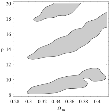
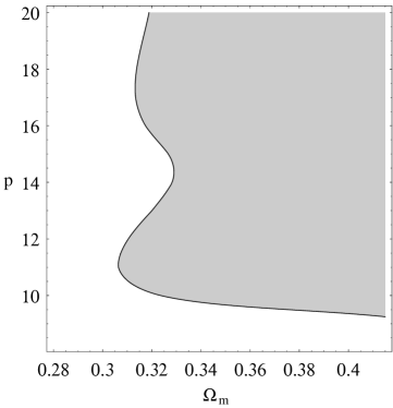
Figure 1: The fitting result of the parameters $\Omega_{m}$ ($l_{0}^{2}$) and $p$. (a) The 68.3% confidence contour plot by using the direct $H(z)$ data in table I. (b) The 68.3% confidence contour plot by using the SNLS data.

We show the deceleration parameter $q$ in figure 2 with best fit values of $\Omega_{m}$ and $p$ by direct $H(z)$ data. Figure 2 illuminates that the universe oscillates between deceleration phase and acceleration phase.

Figure 2: The deceleration parameter $q$ with best fit $\Omega_{m}=0.397$ and $p=11.0$.

III Quantum Stability

A severe problem of any phantom field is quantum stability. In practice, we do not require that the phantom is fundamentally stable, but quasi-stable, which means, its lifetime is larger than the age of the universe. This problem has been discussed in carroll cline . Here we follow the investigations in carroll . The simplest interaction between phantom and graviton takes the form,

$$\phi\rightarrow h+\phi_{1}+\phi_{2}\ ,$$ (41)

where $h$ denotes the gravitational fluctuations on an FRW background, $\phi_{1}$, $\phi_{2}$ represent other two phantom fields. We note here that, though $h$ will be different if we take a Minkowski background, but, the difference is tiny and negligible in the spacetime region we considered for this interaction. Here we consider a series expansion around the initial value of the numerical example we studies above, $\phi(z=0)/\mu=0.022$. Based on the discussion in carroll , we set the interaction term,

$${\mathcal{L}}_{i} = \frac{1}{\mu}(\mu h)\frac{1}{3!}V^{\prime\prime\prime}(\phi_{0})\phi^{3}$$ (42)

$$= A\lambda_{e}(\mu h)\phi^{3}\ ,$$ (44)

Where $\lambda_{e}$ is defined as

$$\lambda_{e}\triangleq\frac{1}{6}\frac{V_{0}}{\mu^{4}}\sin(p\frac{\phi_{0}}{\mu})\sim 10^{-118},$$ (45)

where $p$ takes the best fit value in last section $p=15.3$. Clearly, if we treat phantom as fundamental theory, it will be unstable, and the reaction rate goes to infinity because the volume of the phase space of $\phi$, $\phi_{1}$, $\phi_{2}$ goes to infinity. However, if we treat it as an effective theory which is only valid below some energy scale $\Lambda$, the reaction rate $\Gamma$ becomes,

$$\Gamma\sim\lambda_{e}^{2}\frac{\Lambda^{2}}{m_{\phi}}\ ,$$ (46)

where the effective mass of the phantom $m_{\phi}$ is defined as

$$m_{\phi}\triangleq(-AV^{\prime\prime})^{1/2}\sim p\mu\sqrt{\frac{AV_{0}}{\mu^{4}}}=10^{-60}p\mu A^{1/2}.$$ (47)

Here and the following, we take $A=1$ without special announcement. The phantom field as an effective field is viable if its reaction rate $\Gamma$ is smaller than the present Hubble parameter,

$$\Gamma<H_{0}\sim 10^{-60}\mu,$$ (48)

which means,

$$\lambda_{e}^{2}\frac{\Lambda^{2}}{m_{\phi}}<H_{0},$$ (49)

that is $\Lambda<10^{58}\mu$. In fact, any effective theory is valid at such a high energy scale, which is far beyond our present lab energy scale, surely be a perfect effective theory. But, besides the decay channel as shown in (41), we must consider the cases that one phantom decay into several particles. By summing over all these possibilities, one arrives at the total reaction rate carroll

$$\Gamma_{\rm tot}=\Gamma\left[1-\left(\frac{\Lambda}{\mu}\right)^{2}\right]^{-2}\ .$$ (50)

We see that if $\Lambda$ is smaller than $\mu$, $\Gamma_{\rm tot}$ will keep the same order of $\Gamma$, which is not a stringent constraint.

However, as an effective theory, one must include all possible terms compatible with the symmetry of the Lagrangian up to finite orders to guarantee the renormalizablity of the theory–contributions from high order terms are much suppressed which we can neglect up to required precision. A most famous effective theory is four-fermion interaction theory, as the low effective theory of electro-weak interaction. Expands the propagator of the gauge boson in electro-weak according to the mass of $W$ boson, we see that the derivative coupling appears. Hence a derivative coupling in an effective theory is quite reasonable. We consider the interaction Lagrangian of graviton and phantom, with an approximate global symmetry,

$${\cal L}_{ig}=\frac{\gamma}{\mu^{2}\Lambda^{4}}\left[\mu h(\partial\phi,\partial\phi)\right]^{2}\ ,$$ (51)

where $\gamma$ is a constant of order 1. The reaction rate becomes

$$\Gamma\sim{\gamma^{2}\Lambda^{6}\over m_{\phi}\mu^{2}}\ ,$$ (52)

which should be smaller than the present Hubble parameter. Therefore we reach

$$\Lambda^{6}<\frac{H_{0}m_{\phi}\mu^{4}}{\gamma^{2}}\sim 10^{-120}p\mu^{6}.$$ (53)

The key difference between our result and the result in carroll dwells at the effective mass of the phantom field. In fact, our result the reaction rate $\Gamma$ in (52) is is suppressed by a factor $p$. On the observational side, we see that the 1-$\sigma$ confidence region form a confidence tower, no clear upper bound of $p$. On the theoretical side, one hardly find principles to constrain $p$ in the natural potential in this cosmological context. Physically, the effective mass of the phantom in the present model can be notably larger than $H_{0}=10^{-33}$ eV, which is taken as the mass of the phantom in carroll . For example, if $m_{\phi}=10^{-27}$ eV, which is quite beyond our present abilities of accelerators, $\Lambda$ will exceed 1TeV and hence it is also beyond our present lab energy scale. Thus, the present model is promising due to this suppress mechanism for derivative coupling. Also, we note here that a larger $A$ is helpful to increase the mass of the phantom, which can be seen from (47).

IV Conclusions and discussions

To summarize, this paper illuminates that direct $H(z)$ data is much more efficient than the supernovae for the fine structures of Hubble diagram.

We first put forward a model based on the previous studies on the PNGB. In this model the total fluid in the universe may evolve as phantom in some stages, which contents the direct $H(z)$ data in table I. Then we study its dynamical properties and find its critical points. And we also study the stability about the singularities of this system.

In section II we fit our model by using $H(z)$ data and supernovae data, respectively. The results are quite different, as we expected. Because the sample of $H(z)$ data is too small, the confidence contour is disconnect, which means that we still lack enough information about the oscillations of $H(z)$. We hope the future observations offering more data of $H(z)$ so that we can investigates the history of the universe in a more detail way.

In section III we investigate the stability of the present model. Our treatise is to treat the phantom model as an effective model truncated at some energy scale $\Lambda$. As the previous studies, we find that the coupling to graviton needs a truncate scale much larger than the lab energy scale, if we require the lifetime of the phantom is longer than the universe. Different from the previous studies, we find that the derivative coupling between phantom and graviton is viable due to the special potential of the present model.

Acknowledgments: We thank M. Trodden for discussions on his paper carroll . Our thanks also goes to F. Wang for discussions of the section III. This work was supported by the National Natural Science Foundation of China , under Grant No. 10533010, the Project-sponsored SRF for ROCS, SEM of China, and Program for New Century Excellent Talents in University (NCET).

References

- (1) A. G. Riess et al. , Astron. J. 116, 1009 (1998), astro-ph/9805201; S. Perlmutter et al., Astrophys. J. 517, 565 (1999), astro-ph/9812133.
- (2) Edmund J. Copeland, M. Sami and Shinji Tsujikawa, hep-th/0603057.
- (3) R. Jimenez, L. Verde, T. Treu and D. Stern, Astrophys. J. 593, 622 (2003) [astro-ph/0302560].
- (4) R. Jimenez and A. Loeb, Astrophys. J. 573, 37 (2002) [astro-ph/0106145].
- (5) R. G. Abraham et al. [GDDS Collaboration], Astron. J. 127, 2455 (2004) [astro-ph/0402436]; T. Treu, M. Stiavelli, S. Casertano, P. Moller and G. Bertin, Mon. Not. Roy. Astron. Soc. 308, 1037 (1999); T. Treu, M. Stiavelli, P. Moller, S. Casertano and G. Bertin, Mon. Not. Roy. Astron. Soc. 326, 221 (2001) [astro-ph/0104177]; T. Treu, M. Stiavelli, S. Casertano, P. Moller and G. Bertin, Astrophys. J. Lett. 564, L13 (2002); J. Dunlop, J. Peacock, H. Spinrad, A. Dey, R. Jimenez, D. Stern and R. Windhorst, Nature 381, 581 (1996); H. Spinrad, A. Dey, D. Stern, J. Dunlop, J. Peacock, R. Jimenez and R. Windhorst, Astrophys. J. 484, 581 (1997); L. A. Nolan, J. S. Dunlop, R. Jimenez and A. F. Heavens, Mon. Not. Roy. Astron. Soc. 341, 464 (2003) [astro-ph/0103450].
- (6) J. Simon, L. Verde and R. Jimenez, Phys. Rev. D 71, 123001 (2005) [astro-ph/0412269].
- (7) L. Samushia and B. Ratra, Astrophys. J. 650, L5 (2006) [astro-ph/0607301].
- (8) D. N. Spergel et al., arXiv:astro-ph/0603449.
- (9) R.R. Caldwell, Phys.Lett. B545 (2002) 23, astro-ph/9908168; P. Singh, M. Sami and N. Dadhich, Phys. Rev. D 68, 023522 (2003) [arXiv:hep-th/0305110].
- (10) C. M. Chen, D. V. Galtsov and M. Gutperle, Phys. Rev. D 66, 024043 (2002); P. K. Townsend and M. N. R.Wohlfarth, Phys. Rev. Lett. 91, 061302 (2003).
- (11) E. Elizalde, S. Nojiri and S. D. Odintsov, Phys. Rev. D 70, 043539 (2004).
- (12) S. Nojiri and S. D. Odintsov, Phys. Lett. B 562,2003,147;B. Boisseau, G. Esposito-Farese, D. Polarski, Alexei A. Starobinsky, Phys. Rev. Lett. 85, 2236 (2000);R. Gannouji, D. Polarski, A. Ranquet, A. A. Starobinsky JCAP 0609,016 (2006); Z.K. Guo, R.G. Cai and Y.Z. Zhang, astro-ph/0412624; R. G. Cai and A. Wang, JCAP 0503, 002 (2005) [arXiv:hep-th/0411025]; Z.K. Guo and Y.Z. Zhang, Phys.Rev. D71 (2005) 023501, astro-ph/0411524; Z.K. Guo, Y.S. Piao, X. Zhang and Y.Z. Zhang, Phys.Lett. B608 (2005) 177-182, astro-ph/0410654; S. M. Carroll, A. De Felice and M. Trodden Phys.Rev. D71 (2005) 023525, astro-ph/0408081; S. Nesseris and L. Perivolaropoulos Phys.Rev. D70 (2004) 123529, astro-ph/0410309; Y.H. Wei , gr-qc/0502077; S. Nojiri, S. D. Odintsov and S. Tsujikawa, Phys. Rev. D 71, 063004 (2005) [arXiv:hep-th/0501025]; P. Singh, arXiv:gr-qc/0502086; M.R. Setare, hep-th/0701085; H. Stefancic, arXiv:astro-ph/0504518; V. K. Onemli and R. P. Woodard , Phys. Rev. D70:107301,2004; Class. Quant. Grav. 19 (2002) 4607; gr-qc/0612026.
- (13) Z. K. Guo, Y. S. Piao, X. Zhang and Y. Z. Zhang, arXiv:astro-ph/0608165; B. Feng, X. L. Wang and X. M. Zhang, Phys. Lett. B 607, 35 (2005) [arXiv:astro-ph/0404224]; M. R. Setare, Phys. Lett. B 641, 130 (2006); X. Zhang, Phys. Rev. D 74, 103505 (2006) [arXiv:astro-ph/0609699]; Y. f. Cai, H. Li, Y. S. Piao and X. m. Zhang, arXiv:gr-qc/0609039; M. Alimohammadi and H. M. Sadjadi, arXiv:gr-qc/0608016; H. Mohseni Sadjadi and M. Alimohammadi, Phys. Rev. D 74, 043506 (2006) [arXiv:gr-qc/0605143]; W. Wang, Y. X. Gui and Y. Shao, Chin. Phys. Lett. 23 (2006) 762; X. F. Zhang and T. Qiu, arXiv:astro-ph/0603824; R. Lazkoz and G. Leon, Phys. Lett. B 638, 303 (2006) [arXiv:astro-ph/0602590]; X. Zhang, Commun. Theor. Phys. 44, 762 (2005); P. x. Wu and H. w. Yu, Int. J. Mod. Phys. D 14, 1873 (2005) [arXiv:gr-qc/0509036]; G. B. Zhao, J. Q. Xia, M. Li, B. Feng and X. Zhang, Phys. Rev. D 72, 123515 (2005) [arXiv:astro-ph/0507482]; H. Wei, R. G. Cai and D. F. Zeng, Class. Quant. Grav. 22, 3189 (2005) [arXiv:hep-th/0501160]; H. Wei and R. G. Cai, Phys. Rev. D 72 (2005) 123507 [arXiv:astro-ph/0509328]; H. Wei and R. G. Cai, Phys. Lett. B 634, 9 (2006) [arXiv:astro-ph/0512018]; J. Q. Xia, B. Feng and X. M. Zhang, Mod. Phys. Lett. A 20, 2409 (2005) [arXiv:astro-ph/0411501]; Z. K. Guo, Y. S. Piao, X. M. Zhang and Y. Z. Zhang, Phys. Lett. B 608, 177 (2005) [arXiv:astro-ph/0410654]; B. Feng, M. Li, Y. S. Piao and X. Zhang, Phys. Lett. B 634, 101 (2006) [arXiv:astro-ph/0407432]; X. Zhang and F.Q. Wu, Phys. Rev. D72 (2005) 043524; Y. Cai, H. Li, Y. Piao, and X. Zhang, gr-qc/0609039; R. Lazkoz and G. Leon, Phys. Lett. B 638, 303 (2006) [arXiv:astro-ph/0602590]; W. Zhao, Phys. Rev. D 73 (2006) 123509 [arXiv:astro-ph/0604460]. H. S. Zhang and Z. H. Zhu, Phys. Rev. D 73, 043518 (2006); H. Wei and R. G. Cai, Phys. Rev. D 73, 083002 (2006) R. G. Cai, H. S. Zhang and A. Wang, Commun. Theor. Phys. 44, 948 (2005) [arXiv:hep-th/0505186]. A.A. Andrianov, F. Cannata and A. Y. Kamenshchik, Phys.Rev.D72, 043531,2005; F.Cannata and A. Y. Kamenshchik, , gr-qc/0603129; Pantelis S. Apostolopoulos and Nikolaos Tetradis , Phys. Rev. D 74 (2006) 064021; H. S. Zhang and Z. H. Zhu, Phys. Rev. D 75, 023510 (2007) [arXiv:astro-ph/0611834].
- (14) H. Wei and S. N. Zhang, Phys. Lett. B 644, 7 (2007) [arXiv:astro-ph/0609597];
- (15) K. Freese, J. A. Frieman and A. V. Olinto, Phys. Rev. Lett. 65, 3233 (1990).
- (16) J. A. Frieman, C. T. Hill, A. Stebbins and I. Waga, Phys. Rev. Lett. 75 (1995) 2077; Y. Nomura, T. Watari and T. Yanagida, Phys. Lett. B 484 (2000) 103; J. E. Kim and H. P. Nilles, Phys. Lett. B 553 (2003) 1; K. Choi, Phys. Rev. D 62 (2000) 043509; L. J. Hall, Y. Nomura and S. J. Oliver, astro-ph/0503706; R. Barbieri, L. J. Hall, S. J. Oliver and A. Strumia, hep-ph/0505124.
- (17) S. Dodelson, M. Kaplinghat and E. Stewart, Phys. Rev. Lett. 85, 5276 (2000) [arXiv:astro-ph/0002360].
- (18) Z. L. Yi and T. J. Zhang, astro-ph/0605596, MPLA in press; Puxun Wu, Hongwei Yu, Phys.Lett. B644 (2007) 16.
- (19) P. Astier et al., 2005, Astron.Astrophys. 447 (2006) 31, astro-ph/0510447.
- (20) W. Freedman et al., 2001, Astrophys. J. , 553, 47.
- (21) S. M. Carroll, M. Hoffman and M. Trodden, Phys. Rev. D 68, 023509 (2003) [arXiv:astro-ph/0301273].
- (22) J. M. Cline, S. Jeon and G. D. Moore, Phys. Rev. D 70, 86 043543 (2004).