Astrometric-spectroscopic determination of the absolute masses of the HgMn binary star $\phi$ Herculis

Abstract

The Mercury-Manganese star $\phi$ Her is a well known spectroscopic binary that has been the subject of a recent study by Zavala et al. (2006), in which they resolved the companion using long-baseline interferometry. The total mass of the binary is now fairly well established, but the combination of the spectroscopy with the astrometry has not resulted in individual masses consistent with the spectral types of the components. The motion of the center of light of $\phi$ Her was clearly detected by the Hipparcos satellite. Here we make use of the Hipparcos intermediate data (‘abscissa residuals’) and show that by combining them in an optimal fashion with the interferometry the individual masses can be obtained reliably using only astrometry. We re-examine and then incorporate existing radial-velocity measurements into the orbital solution, obtaining improved masses of $3.05\pm 0.24$ M_☉ and $1.614\pm 0.066$ M_☉ that are consistent with the theoretical mass-luminosity relation from recent stellar evolution models. These mass determinations provide important information for the understanding of the nature of this peculiar class of stars.

1. Introduction

In a recent paper Zavala et al. (2006) reported interferometric observations of the Mercury-Manganese star $\phi$ Her (HD 145389, HR 6023, HIP 79101, $\alpha_{\rm J2000}=16^{\rm h}08^{\rm m}46\fs 18$, $\delta_{\rm J2000}=+44\arcdeg 56\arcmin 05\farcs 7$, spectral type B9:p(HgMn), $V=4.22$), which is a binary star. This object belongs to a class of peculiar non-magnetic B-type stars that show abundance anomalies of several elements, some of which (such as Hg and Mn) can be enhanced by orders of magnitude (Preston, 1974). Depletions of other elements are seen as well. These anomalies are thought to be produced by radiatively-driven diffusion and gravitational settling (Michaud, 1970). The observations of Zavala et al. (2006) spatially resolve the companion of $\phi$ Her for the first time. The object had previously been known as a single-lined spectroscopic binary with a period of about 560 days (Babcock, 1971; Aikman, 1976) and an eccentric orbit. Their interferometric measurements with the Navy Prototype Optical Interferometer (NPOI) allowed Zavala et al. (2006) to measure the brightness of the companion and use it to estimate its spectral type. This, in turn, facilitated their detection of spectral lines of the secondary for the first time in spectra taken at the Dominion Astrophysical Observatory. The secondary was also detected spectroscopically by Dworetsky & Willatt (2006).

The system is therefore technically now double-lined, although as pointed out by Zavala et al. (2006) the handful of secondary radial velocities they were able to measure with great difficulty do not provide a firm constraint on the velocity semiamplitude of that star. Furthermore, they found that the combination of their high-precision interferometric orbit with the elements of the single-lined spectroscopic orbit reported by Aikman (1976) led to absolute masses for the components that are inconsistent with the spectral types. Therefore, although the total mass of the binary is now fairly well known, the individual masses cannot yet be determined dynamically. Such basic properties of the stars are of considerable interest given the chemical peculiarities of this class of objects, which have been the subject of extensive studies of many different kinds (see, e.g., Adelman, Gulliver & Rayle, 2001; Adelman, Adelman & Pintado, 2003; Adelman et al., 2004; Dolk, Wahlgren & Hubrig, 2003; Dworetsky & Budaj, 2000; Leushin, 1995, and references therein).

We were puzzled by this apparent inconsistency between the seemingly precise radial velocities and the astrometry, and we wondered whether other velocity measurements available in the literature might clarify the situation. In addition, $\phi$ Her was observed in the course of the Hipparcos mission (ESA, 1997). Those measurements clearly revealed the motion of the center of light due to the binary orbit, suggesting they could be used to good advantage in the determination of the individual masses. The motivation for this paper is therefore threefold: i) To show how, in the absence of spectroscopy, the astrometric measurements from Hipparcos can indeed be combined with the NPOI observations of Zavala et al. (2006) to yield reliable masses for both stars for the first time, purely astrometrically. This serves as an interesting example of the value of the Hipparcos intermediate data for solving or improving binary orbits and inferring other stellar properties; ii) To readdress the issue of the Aikman (1976) velocities in light of the new solution. We show that those data are not really inconsistent with the astrometry, but do lack critical phase coverage and must be supplemented by other information in order to be useful; iii) To incorporate additional velocity measurements not previously used, in order to further strengthen the orbital solution. The final masses not only have much improved precision, but are consistent with the mass-luminosity relation as given by current stellar evolution models.

2. Interferometric observations

The original NPOI measurements obtained by Zavala et al. (2006) consist of interferometric squared visibilities ($V^{2}$) and closure phases collected on 25 separate nights from 1997 April to 2005 July. The visibilities of each night were combined to infer the angular separation ($\rho$) and position angle ($\theta$) of the binary, and these were subsequently used to derive the elements of the astrometric orbit. The measurements published are $\rho$ and $\theta$, along with the corresponding error ellipses. The residuals from the orbit are only a few tenths of a milli-arc second (mas) in angular separation, and a few tenths of a degree in position angle, indicating the very high precision of those measurements. The orbit has an angular semimajor axis of 32.1 mas, which, when combined with the Hipparcos parallax ($\pi_{\rm Hip}=14.27\pm 0.52$ mas) allowed Zavala et al. (2006) to infer the total mass of the binary as $M_{\rm tot}=4.7\pm 0.6$ M_☉. Additionally, the interferometric measurements yielded the average magnitude difference between the primary and secondary of $\phi$ Her at two wavelengths: $\Delta m$ (5500 Å) $=2.57\pm 0.05$ mag and $\Delta m$ (7000 Å) $=2.39\pm 0.05$ mag. As discussed below this information is key to the mass determinations.

3. Hipparcos observations

The star $\phi$ Her was observed by the Hipparcos satellite during its 37-month astrometric mission under the designation HIP 79101, and was measured a total of 76 times from 1989 December to 1993 March, or a slightly over two orbital cycles of the binary. Each measurement consisted of a one-dimensional position (‘abscissa’) along a great circle representing the scanning direction of the satellite, tied to an absolute frame of reference known as the International Celestial Reference System (ICRS). In addition to providing the trigonometric parallax as well as the position and proper motion of the center of light based on the synthesis of all these measurements (the so-called standard 5-parameter fit), the astrometric solution reported in the Catalogue (ESA, 1997) revealed a perturbation that was modeled as orbital motion, since the binary nature of the object was already known. Several of the orbital elements including the period ($P$), the eccentricity ($e$), and the longitude of periastron of the primary ($\omega_{\rm A}$) were held fixed at the values determined spectroscopically by Aikman (1976) to facilitate the solution, and the other elements were solved for. These included the semimajor axis of the center of light ($a_{\rm phot}=9.09\pm 0.65$ mas), the inclination angle ($i=36\arcdeg\pm 14\arcdeg$), the position angle of the ascending node ($\Omega=188\arcdeg\pm 12\arcdeg$, J2000), and the time of periastron passage ($T$). More recently Jancart et al. (2005) reported a reanalysis of the Hipparcos intermediate data, still adopting $P$, $e$, $\omega_{\rm A}$, as well as $T$ from the spectroscopic work by Aikman (1976), but with the added assumption that the secondary contributes no light to the system. This provides a connection between the measured semimajor axis $a_{\rm phot}$ and the radial velocity semiamplitude $K_{\rm A}$, which was adopted also from Aikman (1976). Their results for the inclination ($i=10\fdg 3\pm 0\fdg 7$) and especially the position angle of the node ($\Omega=148\fdg 3\pm 3\fdg 0$) are quite different from the Hipparcos solution, but we now know from the detection of the secondary by Zavala et al. (2006) that this star does contribute some light, so the assumption of Jancart et al. (2005) is not a good one in this particular case.

As it turns out, the information provided by the Hipparcos data is complementary to that given by the ground-based interferometry, and as we show below the combination of the two allows the individual masses of $\phi$ Her to be determined independently of any assumptions, and independently also of any spectroscopic information. Since some of the orbital elements reported by Zavala et al. (2006) are much improved compared to Aikman (1976), a reanalysis of the Hipparcos data with those constraints would therefore seem to be in order. Better still, the Hipparcos data can be combined directly with the NPOI observations in a simultaneous least-squares solution yielding all the elements at once. This is the path we follow in the next section. The intermediate data from Hipparcos are available in the form of one-dimensional ‘abscissa residuals’, which are the residuals from the standard 5-parameter solutions published in the Catalogue (ESA, 1997). By extending the 5-parameter model to include orbital motion, as done by the Hipparcos team, these observations can be used to strengthen the combined solution. The nominal errors of these measurements have a median of 1.85 mas.

4. Combined orbit and stellar masses

Long-baseline interferometry provides information on the relative orbit of the binary (with semimajor axis $a$) as well as the brightness difference, whereas the Hipparcos observations refer to the motion of the center of light of the binary relative to the barycenter (with semimajor axis $a_{\rm phot}$), on an absolute frame of reference. The two kinds of measurements are redundant to some extent because they both constrain the elements $P$, $e$, $i$, $\omega_{\rm A}$, $\Omega$, and $T$. Their simultaneous use in a global fit is therefore expected to lead to a more robust solution. The use of the Hipparcos measurements introduces several other parameters that must be solved for at the same time, including corrections to the catalog values of the position of the barycenter ($\Delta\alpha^{*}$, $\Delta\delta$) at the mean reference epoch of 1991.25, and corrections to the proper motion components ($\Delta\mu_{\alpha}^{*}$, $\Delta\mu_{\delta}$) and to the parallax ($\Delta\pi_{\rm Hip}$). The formalism for modeling the abscissa residuals follows closely that described by van Leeuwen & Evans (1998), Pourbaix & Jorissen (2000), and Jancart et al. (2005), including the correlations between measurements from the two independent data reduction consortia that processed the original Hipparcos observations (ESA, 1997). The details are reviewed in the Appendix. With the inclusion of the semimajor axes $a$ and $a_{\rm phot}$ there are 13 unknowns altogether. We solve for them simultaneously using standard non-linear least-squares techniques (Press et al., 1992, p. 650). In the course of the iterations we noticed that one of the NPOI observations (taken on 2004 July 21) gave an unusually large residual in both angular separation ($+0.86$ mas, or $3.2\sigma$) and position angle ($-1\fdg 16$, or $4.1\sigma$). The same observation stands out in the solution by Zavala et al. (2006) with similar residuals, and is one of several measurements taken at nearly the same orbital phase, so is not particularly critical. We have elected to exclude it from the solution. The relative weights between the NPOI and Hipparcos observations were assigned according to their individual errors. Since internal errors are not always realistic, we adjusted them by applying a scale factor in such a way as to achieve a reduced $\chi^{2}$ value near unity separately for each type of observation. This was done by iterations. A similar procedure was followed by Zavala et al. (2006). This resulted in scale factors of 0.34 and 0.24 for the NPOI angular separations and position angles, and 0.84 for the Hipparcos measurements.

The results of this fit are given in Table 1 under the heading NPOI+Hipparcos. For reference we include also the spectroscopic solution reported by Aikman (1976), the fit by Zavala et al. (2006), and the constrained solution by the Hipparcos team. The position angle of the node given by Zavala et al. (2006) requires a change of quadrant to conform to the usual convention that the ascending node ($\Omega$) corresponds to the node at which the secondary is receding from the observer. The orbital elements from our fit are generally seen to be consistent with those of Zavala et al. (2006) (whose solution combines interferometry with radial velocities), but with considerably smaller uncertainties.

The projection of the photocentric orbit on the plane of the sky along with a schematic representation the Hipparcos measurements is seen in Figure 1, where the axes are parallel to the right ascension and declination directions. Because these measurements are one-dimensional in nature, their exact location on the plane of the sky cannot be shown graphically. The filled circles represent the predicted location on the computed orbit. The dotted lines connected to each filled circle indicate the scanning direction of the Hipparcos satellite for each measurement, and show which side of the orbit the residual is on. The length of each dotted line represents the magnitude of the $O\!-\!C$ residual. The short line segments at the end of and perpendicular to the dotted lines indicate the direction along which the actual observation lies, although the precise location is undetermined. Occasionally more than one measurement was taken along the same scanning direction, in which case two or more short line segments appear on the same dotted lines. The orbit is counterclockwise (direct). The path of $\phi$ Her on the plane of the sky as seen by Hipparcos is shown in Figure 2. The contorted pattern results from the combination of annual proper motion (indicated by the arrow), parallactic motion, and orbital motion.

In addition to providing the parallax, the key contribution of the Hipparcos observations regarding the masses of $\phi$ Her is that they allow the measurement of the semimajor axis of the photocenter. This parameter can be expressed in terms of the relative semimajor axis (e.g., van de Kamp, 1967) as $a_{\rm phot}=a(B-\beta)$, where $B$ is the mass fraction $M_{\rm B}/(M_{\rm A}+M_{\rm B})$ and $\beta$ is the light fraction $\ell_{\rm B}/(\ell_{\rm A}+\ell_{\rm B})$. This can be put in a more convenient form as

$$a_{\rm phot}=a\left({q\over 1+q}-{1\over 1+10^{0.4\Delta m}}\right),$$ (1)

where $q\equiv M_{\rm B}/M_{\rm A}$ and $\Delta m$ is the magnitude difference in the Hipparcos passband ($H_{p}$). Therefore, if the magnitude difference is known, the combination of both kinds of astrometric measurements allows one to solve for the mass ratio $q$. Since the total mass can also be determined from Kepler’s Third Law given the parallax ($\pi_{\rm Hip}$), the individual masses in units of the solar mass follow immediately:

$$M_{\rm A} = {a^{3}\over\pi_{\rm Hip}^{3}P^{2}}\left(1-{a_{\rm phot}\over a}-{1\over 1+10^{0.4\Delta m}}\right)$$ (2)

$$M_{\rm B} = {a^{3}\over\pi_{\rm Hip}^{3}P^{2}}\left({a_{\rm phot}\over a}+{1\over 1+10^{0.4\Delta m}}\right).$$ (3)

In the above expressions all angular quantities are expressed in the same units, and the period is in units of sidereal years. The interferometric measurement of $\Delta m$ by Zavala et al. (2006) is therefore of crucial importance here, and we have made use of it as an external constraint (along with its uncertainty) in order to solve for the masses. Strictly speaking, however, the value entered in the equations above must correspond to the same passband as the Hipparcos observations ($H_{p}$), whereas the relevant $\Delta m$ reported by Zavala et al. (2006) corresponds to the passband of one of the spectral channels of the NPOI centered at 5500 Å. We have assumed that the latter corresponds closely to the visual band, and we have applied a small correction to transform it to the $H_{p}$ band using the relations by Harmanec (1998). This transformation depends on the individual $U\!-\!B$ and $B\!-\!V$ colors of the components, which have not been measured directly. But as described in §7, they can be estimated using stellar evolution models (see Table 5 below). The result is then $\Delta H_{p}=2.669\pm 0.051$, where the uncertainty includes the contribution from the scatter of the transformation.

The individual masses we obtain for the components of $\phi$ Her are reported in Table 1, along with other quantities derived from the orbital elements, such as the velocity amplitudes ($K_{\rm A}$, $K_{\rm B}$) predicted for the primary and secondary. The uncertainties in the derived quantities account for the correlations between the various elements. The total mass is essentially the same as derived by Zavala et al. (2006), but with a significantly reduced error due mostly to the improved parallax. However, our individual masses are different than the nominal values they inferred, and are much closer to those expected for the spectral types estimated by them (see below). We emphasize that our mass determinations in this section are purely astrometric, since we have not made any use of the spectroscopy in our fit. Several of the orbital elements are considerably more precise in our solution than in the work of Zavala et al. (2006), including the semimajor axis $a$ that in principle depends only on the NPOI observations, which are common to both fits. This is most likely due to two factors: our rejection of one of the NPOI observations giving large residuals, and the fact that we did not use the radial-velocity observations of Aikman (1976), which appear to show some inconsistency with the astrometry and may be biasing the solution of Zavala et al. (2006) causing larger errors. We investigate this issue in more detail in the next section. Our error in the period is also smaller despite the shorter time span of the observations considered in our fit (15.5 yr) compared to theirs (40.2). We attribute this to the same reasons.

5. The radial velocities of $\phi$ Her

The orbital solution of Zavala et al. (2006) is a combined fit of their NPOI data with the radial velocities from Aikman (1976). Although this resulted in orbital elements with significantly smaller errors, they instead elected to use the mass function as computed originally by Aikman (1976), and with their total system mass of 4.7 M_☉ they inferred individual masses of 3.6 M_☉ for the primary and 1.1 M_☉ for the secondary. They correctly pointed out that these values seem anomalous for the spectral types (which they estimated as B8V and A8V), the primary mass being too large and the secondary too small. Since the secondary mass is proportional to $P^{1/3}M_{\rm tot}^{2/3}\sqrt{1-e^{2}}K_{\rm A}/\sin i$, the two main factors that contribute to the discrepancy appear to be the larger inclination angle of Zavala et al. (2006) compared to ours, and the smaller velocity semiamplitude. Given that the difference in the inclination angle is not sufficient to explain the problem, we conclude that the $K_{\rm A}$ value from Aikman (1976) is probably too small.

In Figure 3 we compare the original radial velocities by Aikman (1976) with our astrometric solution from the previous section (indicated with the solid line), in which the center-of-mass velocity has been adjusted by eye to fit the velocities. It is seen that the agreement is very good with the exception of one measurement obtained precisely at the descending node near phase 0.0, which shows a residual $\sim$5 times larger than the scatter of the remaining points. This measurement happens to carry the highest weight for establishing the semiamplitude $K_{\rm A}$, and we speculate that it may be biased and may be pulling the amplitude toward lower values. For reference we show also the original solution by Aikman (1976) (dotted line), in which the amplitude is lower and that measurement does not particularly stand out as an outlier. A new spectroscopic solution without this observation gives a larger semiamplitude ($K_{\rm A}=2.68\pm 0.20$ km s^-1), as expected, although it is also a bit more uncertain because of the lack of constraint at the maximum. We note that several of the other elements in this trial solution are also closer to our results in §4, particularly the eccentricity ($e=0.516\pm 0.036$) and the longitude of periastron ($\omega_{\rm A}=355\fdg 6\pm 3\fdg 5$), which is suggestive.

A search for other velocities of $\phi$ Her in the literature revealed a set of measurements of the primary star obtained by Adelman, Gulliver & Rayle (2001) between 1989 and 1998 that appears to be of good quality, and that was not used in the work of Zavala et al. (2006). Examination of those data shows that unfortunately they too lack coverage near the all-important descending node, and in addition there are two outliers. Nevertheless, we believe them to be potentially useful so we have considered them along with those of Aikman (1976) in a new combined orbital solution described next. The velocities of the secondary measured by Zavala et al. (2006), on the other hand, are of insufficient quality to be of use and show very poor agreement with our astrometric solution.

6. New combined solution and revised masses

The inclusion of radial velocities in the fit along with the astrometry introduces a redundancy from the fact that the velocity semiamplitude is constrained by both kinds of measurements. In addition to the 13 adjustable quantities considered previously, we add the center-of-mass velocity ($\gamma$) and a velocity offset ($\Delta RV$) to account for a possible difference in the zero points of the two radial velocity data sets. Furthermore, since the velocities provide an indirect constraint on $\Delta m$ through eq.[1] (see below), we now consider $\Delta m$ also as an adjustable quantity instead of as a fixed constraint, and the value of the magnitude difference from interferometry (properly corrected to the $H_{p}$ passband) is regarded as a measurement with its corresponding uncertainty. The scale factor for the Aikman (1976) internal errors was found to be 1.77, and the Adelman, Gulliver & Rayle (2001) velocities were assigned uncertainties of 0.47 km s^-1 so that their reduced $\chi^{2}$ is near unity.

The results of this 16-parameter global solution are listed in the last column of Table 1. The changes compared to the previous fit are generally well within the errors, a sign that the spectroscopic observations we have added are consistent with the astrometry. The rms residuals for an observation of unit weight (NPOI $\rho$ and $\theta$, radial velocities, Hipparcos) are, respectively, $\epsilon_{\rho}=0.13$ mas, $\epsilon_{\theta}=0\fdg 14$, $\epsilon_{\rm RV1}=0.25$ km s^-1, $\epsilon_{\rm RV2}=0.47$ km s^-1, and $\epsilon_{\rm Hip}=1.8$ mas. The individual Hipparcos measurements and $O\!-\!C$ residuals are listed in Table 2. In Figure 4b we show these residuals as a function of orbital phase. The $O\!-\!C$ residuals from the original orbital solution by the Hipparcos team are overplotted in the same figure (open circles), and the two distributions are seen to be essentially the same. For reference, Figure 4a shows the Hipparcos measurements on the same scale before accounting for orbital motion, i.e., the abscissa residuals from the standard 5-parameter solution. The improvement brought about by the orbital fit is obvious. Minor systematics at the level of a few milli-arc seconds remain in the $O\!-\!C$ residuals of Figure 4b, for example near phase 0.7, which we believe may be reflecting the limitations of this data set. The residuals from the NPOI observations are quite similar to those reported by Zavala et al. (2006) and are not repeated here. The velocity residuals are given in Table 3 and Table 4, along with the original measurements; observations that were rejected as described above have their residuals indicated in parentheses. These data are compared graphically in Figure 5 against the computed velocity curve from our fit. As an interesting test on the indirect constraint provided by the velocities on the magnitude difference through other elements, we carried out another solution in which the magnitude difference from interferometry is ignored. This fit gives $\Delta H_{p}=3.00\pm 0.64$ mag, which is not far from the measured value of $2.669\pm 0.051$ mag.

7. Comparison with stellar evolution models

As mentioned earlier the individual masses derived here for the components of $\phi$ Her are in good agreement with those expected for the spectral types of the stars. A more stringent comparison may be made against current stellar evolution models, for example in the mass-luminosity (or mass-absolute magnitude) plane. The absolute magnitudes of the stars in the visual band follow from the system magnitude ($V=4.220\pm 0.025$; Mermilliod & Mermilliod, 1994), the magnitude difference determined interferometrically ($\Delta V=2.57\pm 0.05$), and our revised parallax ($\pi_{\rm Hip}^{\prime}=14.34\pm 0.35$ mas), which corresponds to a distance of $69.7\pm 1.7$ pc. Ignoring extinction we obtain $M_{V}^{\rm A}=0.100\pm 0.059$ and $M_{V}^{\rm B}=2.670\pm 0.074$. In Figure 6a we show the measurements against several model isochrones from the Yonsei-Yale series by Yi et al. (2001) (see also Demarque et al., 2004) for ages between 100 Myr and 400 Myr and solar composition. The agreement is excellent, and we infer an age of $250\pm 100$ Myr from this crude comparison. The assumption of solar composition here is arbitrary, and in fact a number of detailed analyses of the chemical compositon of $\phi$ Her in the literature have generally indicated an iron abundance above solar. For example, the recent study by Zavala et al. (2006) gave a value close to [Fe/H] = +0.2. This, however, refers strictly to the photospheric composition, which is known to be peculiar in $\phi$ Her and other HgMn stars. In these objects some of the elements are enhanced by very large factors (up to $10^{5}$) compared to the Sun, presumably due to radiatively-driven diffusion and gravitational settling (Michaud, 1970). Therefore, the interior composition (which is the relevant quantity for the comparison with models) may be inaccessible to the observer in this class of stars, except perhaps through the study of stellar oscillations, should they be detected.

This apparent difficulty has motivated us to turn the argument around and explore the possibility of inferring the metallicity (as well as the evolutionary age) from the available observational constraints via a more systematic comparison with the models, as described below. In addition to the individual masses and absolute visual magnitudes, we have considered as constraints the integrated colors of the system, which are among the easiest quantities to measure accurately. The observed $B\!-\!V$ index of $\phi$ Her as reported by Mermilliod & Mermilliod (1994) is $-0.070\pm 0.005$ (mean of 46 individual ground-based measurements). On the other hand the Hipparcos Catalogue gives the considerably redder value $-0.045\pm 0.003$, based on the $B_{\rm T}$ and $V_{\rm T}$ measurements from the Tycho experiment onboard the satellite along with a conversion to the Johnson system. These later measurements were superseded by the re-reduction that resulted in the Tycho-2 Catalogue (Høg et al., 2000), according to which $B_{\rm T}=4.155\pm 0.014$ and $V_{\rm T}=4.216\pm 0.009$. Based on these revised values and the conversion to the Johnson system described in the Hipparcos Catalogue (ESA, 1997, Vol. 1, Sect. 1.3) we obtain $B\!-\!V=-0.055\pm 0.014$. This is still redder than the ground-based average, although the uncertainty is perhaps more realistic so that the two determinations are now consistent within the errors. The weighted average, which we adopt in the following, is $\langle B\!-\!V\rangle=-0.068\pm 0.008$. The $U\!-\!B$ color of $\phi$ Her as reported by Mermilliod & Mermilliod (1994) is $U\!-\!B=-0.250\pm 0.009$, from the mean of 40 individual ground-based observations.

To compare the six measured properties ($M_{\rm A}$, $M_{\rm B}$, $M_{V}^{\rm A}$, $M_{V}^{\rm A}$, $U\!-\!B$, $B\!-\!V$) against evolutionary models, we computed by interpolation a large grid of Yonsei-Yale isochrones spanning a wide range of ages (50 to 500 Myr) and metallicities ($-0.50$ to +0.60 in [Fe/H]). Along each isochrone we interpolated the colors and magnitudes of stars in a fine grid of masses over intervals of $\pm$1$\sigma$ centered on our measured values of $M_{\rm A}$ and $M_{\rm B}$. For all combinations of a primary and secondary mass taken from these two intervals we calculated the theoretical integrated colors of the system, and recorded all combinations of the isochrone age and metallicity that yielded simultaneous agreement with the measured individual absolute magnitudes and combined $U\!-\!B$ and $B\!-\!V$ indices, within their uncertainties. Figure 7 displays all consistent models in the age/metallicity plane, where the point size is related to the goodness of fit as measured by the distance $D^{2}$ between the model and the observations in the six-dimensional parameter space,

$$D^{2} = \left[\Delta M_{\rm A}\right]^{2}+\left[\Delta M_{\rm B}\right]^{2}+\left[\Delta M_{V}^{\rm A}\right]^{2}+\left[\Delta M_{V}^{\rm B}\right]^{2}+$$

$$+ \left[\Delta(U\!-\!B)\right]^{2}+\left[\Delta(B\!-\!V)\right]^{2}.$$

Age and metallicity are seen to be highly correlated. The best match with the observations occurs near the middle of the distribution for a composition very near solar ([Fe/H] $=-0.03$) and an age of 210 Myr. The individual masses preferred by this model are within 0.4$\sigma$ of the measured values, the agreement with the individual absolute magnitudes is virtually perfect, and that with the integrated colors is $\sim$0.1$\sigma$. In Table 5 we list the predicted properties from this model along with the measured values. The individual $U\!-\!B$ and $B\!-\!V$ colors for the components are the ones used in §4 to convert the interferometric magnitude difference $\Delta V$ into $\Delta H_{p}$. The best-fit isochrone is shown in Figure 6b. Based on this comparison one may conclude that the interior composition of $\phi$ Her is not significantly different from solar, which is more or less as expected for a young early-type system such as this. We point out, however, that this relies on the colors of $\phi$ Her being normal and also on the colors predicted by the stellar evolution models being realistic. Theoretical colors are unlikely to be in error by significant amounts, but we do note that there are some indications of anomalies in the spectrophotometry of HgMn stars (see, e.g., Adelman, 1984; Adelman, Adelman & Pintado, 2003, and references therein) of a nature similar to those seen in metallic-line A stars and other chemically peculiar objects, which are thought to be connected with line blanketing, particularly in the bluer spectral regions.

8. Concluding remarks

The orbital solutions in §4 and §6 provide an interesting illustration of the usefulness of the Hipparcos intermediate data as a valuable complement to other astrometric or spectroscopic observations. The abscissa residuals from the satellite mission are publicly available for many thousands of binary stars distributed over the entire sky, and although a number of studies have appeared over the past few years that do take advantage of them, this is largely still an underutilized resource. In the case of the HgMn star $\phi$ Her the Hipparcos measurements are key to establishing the individual masses of the components, the most fundamental of the stellar properties. We find good agreement between these masses and the magnitudes and colors of the system and current stellar evolution models, suggesting the bulk composition of the object is near solar. Although the faint secondary has now been detected, both interferometrically and spectroscopically, an accurate measurement of its radial velocity over the orbital cycle should help considerably for reducing the mass uncertainties, which are currently at the 8% and 4% level for the primary and secondary, respectively.

Appendix A Making use of the Hipparcos intermediate observations in the orbital solution of $\phi$ Her

The intermediate data provided with the Hipparcos catalog are the “abscissa residuals”, $\Delta v$, which represent the difference between the satellite measurements (abscissae) along great circles and the predicted abscissae computed from the 5 standard astrometric parameters. The standard parameters are the position of the object ($\alpha_{0}^{*}$, $\delta_{0}$) at the reference epoch $t_{0}=1991.25$, the proper motion components ($\mu_{\alpha}^{*}$, $\mu_{\delta}$), and the parallax ($\pi_{\rm Hip}$). We follow here the notation in the Hipparcos catalog and define $\alpha_{0}^{*}\equiv\alpha_{0}\cos\delta$ and $\mu_{\alpha}^{*}\equiv\mu_{\alpha}\cos\delta$, to include the projection factors. The goal of incorporating an orbital model into the analysis of the Hipparcos data is to reduce the original abscissa residuals to values below those obtained from the 5-parameter solution by taking into account the orbital motion of the photocenter. The $\chi^{2}$ minimization approach for doing this has been described previously by van Leeuwen & Evans (1998), Pourbaix & Jorissen (2000), Jancart et al. (2005), and others. We review the procedure here with additional details to facilitate its application in other cases. Following Pourbaix & Jorissen (2000) the $\chi^{2}$ sum can be represented quite generally as $\chi^{2}=\mbox{\boldmath$\Xi^{t}~{}V^{-1}~{}\Xi$}$, where

$$\mbox{\boldmath$\Xi$}=\mbox{\boldmath$\Delta v$}-\sum_{k=1}^{M}{\partial\mbox{\boldmath$v$}\over\partial p_{k}}\Delta p_{k}$$ (A1)

and $\Xi^{t}$ is the transpose of $\Xi$. In this expression $\Delta v$ is the array of N abscissa residuals provided by Hipparcos, and $\partial\mbox{\boldmath$v$}/\partial p_{k}$ is the array of partial derivatives of the abscissae with respect to the $k$th fitted parameter. The number $M$ of parameters fitted to the astrometry in our case is 12: the 5 standard Hipparcos parameters ($p_{1}=\alpha_{0}^{*}$, $p_{2}=\delta_{0}$, $p_{3}=\mu_{\alpha}^{*}$, $p_{4}=\mu_{\delta}$, $p_{5}=\pi_{\rm Hip}$) and 7 orbital elements ($a_{\rm phot}$, $P$, $e$, $i$, $\omega_{\rm A}$, $\Omega$, $T$, represented as $p_{k}$ with $k=6,\ldots,12$). Here $V^{-1}$ is the inverse of the covariance matrix of the observations, containing the abscissa uncertainties and correlation coefficients (ESA, 1997, Vol. 3, eqs. 17-10 and 17-11). These are both provided in the Hipparcos catalog for each observation. Correlations arise because the same original satellite data were reduced independently by two data reduction consortia (FAST and NDAC; see ESA, 1997), and the results from both are typically included in all solutions. To be explicit,

$$V=\left(\begin{array}[]{cccc}V_{1}&0&\ldots&0\\ 0&V_{2}&\ddots&\vdots\\ \vdots&\ddots&\ddots&0\\ 0&\ldots&0&V_{n}\end{array}\right)$$

where each subarray $V_{j}$ corresponds to a pair of FAST/NDAC measurements (F/N) and is given by

$$\mbox{\boldmath$V_{j}$}=\left(\begin{array}[]{cc}\sigma_{\rm F}^{2}&\rho\sigma_{\rm F}\sigma_{\rm N}\\ \rho\sigma_{\rm F}\sigma_{\rm N}&\sigma_{\rm N}^{2}\end{array}\right)_{j}$$ (A2)

in which $\sigma_{\rm F}$ and $\sigma_{\rm N}$ are the corresponding uncertainties and $\rho$ is the correlation coefficient.

The partial derivatives $\partial\mbox{\boldmath$v$}/\partial p_{k}$ for $k=1$ to 5 in equation (A1) are given in the Hipparcos catalog along with the abscissa residuals. The remaining derivatives can be expressed in terms of the partial derivatives of $v$ with respect to $\alpha_{0}^{*}$ and $\delta_{0}$. These are (ESA, 1997, Vol. 3, eq. 17-15)

$${\partial\mbox{\boldmath$v$}\over\partial p_{k}}={\partial\mbox{\boldmath$v$}\over\partial\alpha_{0}^{*}}{\partial\xi\over\partial p_{k}}+{\partial\mbox{\boldmath$v$}\over\partial\delta_{0}}{\partial\eta\over\partial p_{k}}~{}~{},~{}~{}k=6,\ldots,12,$$ (A3)

in which $\xi$ and $\eta$ are the rectangular coordinates of the photocenter relative to the center of mass of the binary on the plane tangent to the sky at ($\alpha_{0}^{*}$, $\delta_{0}$). The general expressions for these are

$$\xi = \alpha_{0}^{*}+\mu_{\alpha}^{*}(t-t_{0})+P_{\alpha}\pi_{\rm Hip}+\Delta X$$

$$\eta = \delta_{0}+\mu_{\delta}(t-t_{0})+P_{\delta}\pi_{\rm Hip}+\Delta Y$$

in which $P_{\alpha}$ and $P_{\delta}$ are the parallactic factors. Only the last term in each of these equations is relevant in our case. They represent the right ascension and declination components of the orbital motion, and are conveniently expressed as $\Delta X=Bx+Gy$ and $\Delta Y=Ax+Fy$. Here $x$ and $y$ are the rectangular coordinates in the unit orbit given by $x=\cos E-e$ and $y=\sqrt{1-e^{2}}\sin E$, with $E$ being the eccentric anomaly. This angle is related to the period and time of periastron passage through Kepler’s equation, $E-e\sin E=2\pi(t-T)/P$. The symbols $A$, $B$, $F$, and $G$ are the classical Thiele-Innes constants (see, e.g., van de Kamp, 1967), which depend only on the orbital elements $a_{\rm phot}$, $i$, $\omega_{\rm A}$, and $\Omega$, and are given by

$$B = -a_{\rm phot}(\cos\omega_{\rm A}\sin\Omega+\sin\omega_{\rm A}\cos\Omega\cos i)$$

$$A = -a_{\rm phot}(\cos\omega_{\rm A}\cos\Omega-\sin\omega_{\rm A}\sin\Omega\cos i)$$

$$G = -a_{\rm phot}(-\sin\omega_{\rm A}\sin\Omega+\cos\omega_{\rm A}\cos\Omega\cos i)$$

$$F = -a_{\rm phot}(-\sin\omega_{\rm A}\cos\Omega-\cos\omega_{\rm A}\sin\Omega\cos i)$$

The negative sign preceding $a_{\rm phot}$ in these equations reflects our use for this particular application of the longitude of periastron for the primary ($\omega_{\rm A}$) instead of that of the secondary ($\omega_{\rm B}$), for consistency with the elements of the spectroscopic orbit. The customary form of the Thiele-Innes constants in solving the relative orbit of a visual binary uses $\omega_{\rm B}$. Trivially the two angles differ by 180°.

As described by Pourbaix & Jorissen (2000), the nature of the orbital solution is such that of the seven derivatives in equation (A3) the only one that needs to be considered explicitly is the derivative with respect to the semimajor axis, $\partial\mbox{\boldmath$v$}/\partial p_{6}=\partial\mbox{\boldmath$v$}/\partial a_{\rm phot}$. The expression for $\Xi$ in equation (A1) then reduces to

$$\mbox{\boldmath$\Xi$}=\mbox{\boldmath$\Delta v$}-\sum_{k=1}^{5}{\partial\mbox{\boldmath$v$}\over\partial p_{k}}\Delta p_{k}-\left({\partial\mbox{\boldmath$v$}\over\partial\alpha_{0}^{*}}{\partial\xi\over\partial a_{\rm phot}}+{\partial\mbox{\boldmath$v$}\over\partial\delta_{0}}{\partial\eta\over\partial a_{\rm phot}}\right)a_{\rm phot}~{}.$$

The remaining six orbital elements ($P$, $e$, $i$, $\omega_{\rm A}$, $\Omega$, and $T$) do not appear explicitly but are hidden in $\partial\xi/\partial a_{\rm phot}=\partial(\Delta X)/\partial a_{\rm phot}$ and $\partial\eta/\partial a_{\rm phot}=\partial(\Delta Y)/\partial a_{\rm phot}$. Thus, 12 parameters enter the evaluation of $\chi^{2}$ and are to be adjusted to seek its minimum: six are explicit ($a_{\rm phot}$ and $\Delta p_{k}$, with $k=1,\ldots,5$), and the remaining six are implicit.

At each iteration towards the $\chi^{2}$ minimum the array of $O\!-\!C$ residuals $\Xi$ is properly weighted by accounting for the error of each abscissa residual and the correlation between the FAST and NDAC measurements, which typically come in pairs. Representing one of such pairs by $\mbox{$\mathbf{\Xi}$}_{j}=\left(r_{\rm F},r_{\rm N}\right)_{j}$, it is easy to see using the definition of $V_{j}$ above that the corresponding $j$th term $\mbox{$\mathbf{\Xi}$}^{t}_{j}$ $V_{j}^{-1}$ $\mbox{$\mathbf{\Xi}$}_{j}$ in the $\chi^{2}$ sum will be

$${1\over 1-\rho^{2}}\left[\left({r_{\rm F}\over\sigma_{\rm F}}\right)^{2}-{2\rho r_{\rm F}r_{\rm N}\over\sigma_{\rm F}\sigma_{\rm N}}+\left({r_{\rm N}\over\sigma_{\rm N}}\right)^{2}\right]~{}.$$

If for some reason a measurement for only one consortium is available on a certain date (i.e., the observations are not paired for that particular orbit of the Hipparcos satellite), the correlation coefficient is zero and the $\chi^{2}$ term reduces to $(r_{\rm F}/\sigma_{\rm F})^{2}$ or $(r_{\rm N}/\sigma_{\rm N})^{2}$.

Table 1Orbital solutions for $\phi$ Her.

	Aikman (1976)	Zavala et al. (2006)		This paper	This paper
Parameter	(RVs)	(NPOI+RVs)	Hipparcos	(NPOI+Hipparcos)	(NPOI+Hipparcos+RVs)
Adjusted quantities
$P$ (days)	560.5 $\pm$ 1.700	564.69 $\pm$ 0.1300	560.5	564.783 $\pm$ 0.04800	564.834 $\pm$ 0.03800
$\gamma$ (km s-1)	$-16.79$ $\pm$ 0.06+0	$-16.66$ $\pm$ 0.05+0	$\cdots$	$\cdots$	$-16.642$ $\pm$ 0.0450+
$\Delta RV$ (km s-1)	$\cdots$	$\cdots$	$\cdots$	$\cdots$	$-0.41$ $\pm$ 0.12+
$K_{\rm A}$ (km s-1)	2.39 $\pm$ 0.12	2.5	$\cdots$	3.02 $\pm$ 0.28	2.772 $\pm$ 0.073
$e$	0.47 $\pm$ 0.03	0.522 $\pm$ 0.004	0.47	0.5250 $\pm$ 0.0011	0.52614 $\pm$ 0.00086
$\omega_{\rm A}$ (deg)	357 $\pm$ 500	351.9 $\pm$ 2.700	357	355.0 $\pm$ 4.400	350.8 $\pm$ 1.400
$T$ (HJD$-$2,400,000)	string50053.7 $\pm$ 5.5string	50121.8 $\pm$ 1.0string	string50114 $\pm$ 16string	50121.68 $\pm$ 0.25string	50121.43 $\pm$ 0.20string
$i$ (deg)	$\cdots$	12.1 $\pm$ 2.90	36 $\pm$ 14	9.80 $\pm$ 0.77	9.10 $\pm$ 0.40
$\Omega_{\rm J2000}$ (deg)	$\cdots$	string189.1 $\pm$ 2.500	188 $\pm$ 120	186.2 $\pm$ 4.400	190.4 $\pm$ 1.400
$a$ (mas)	$\cdots$	32.1 $\pm$ 0.20	$\cdots$	32.045 $\pm$ 0.0350	32.027 $\pm$ 0.0280
$a_{\rm phot}$ (mas)	$\cdots$	$\cdots$	9.09 $\pm$ 0.65	8.67 $\pm$ 0.39	8.57 $\pm$ 0.36
$\Delta\alpha^{*}$ (mas)	$\cdots$	$\cdots$	$\cdots$	+0.45 $\pm$ 0.32+	+0.44 $\pm$ 0.32+
$\Delta\delta$ (mas)	$\cdots$	$\cdots$	$\cdots$	$-0.58$ $\pm$ 0.43+	$-0.52$ $\pm$ 0.42+
$\Delta\mu_{\alpha}^{*}$ (mas yr-1)	$\cdots$	$\cdots$	$\cdots$	$-0.17$ $\pm$ 0.32+	$-0.15$ $\pm$ 0.32+
$\Delta\mu_{\delta}$ (mas yr-1)	$\cdots$	$\cdots$	$\cdots$	+0.01 $\pm$ 0.35+	+0.03 $\pm$ 0.34+
$\Delta\pi_{\rm Hip}$ (mas)	$\cdots$	$\cdots$	$\cdots$	+0.02 $\pm$ 0.36+	+0.07 $\pm$ 0.35+
$\Delta m$ (mag)	$\cdots$	2.57 $\pm$ 0.05	$\cdots$	2.669 $\pm$ 0.051	2.672 $\pm$ 0.052
Derived quantities
$K_{\rm B}$ (km s-1)	$\cdots$	8.1	$\cdots$	5.62 $\pm$ 0.49	5.23 $\pm$ 0.29
$M_{\rm A}$ (M☉)	$\cdots$	3.6	$\cdots$	3.07 $\pm$ 0.25	3.05 $\pm$ 0.24
$M_{\rm B}$ (M☉)	$\cdots$	1.1	$\cdots$	1.647 $\pm$ 0.075	1.614 $\pm$ 0.066
$q\equiv M_{\rm B}/M_{\rm A}$	$\cdots$	0.31	$\cdots$	0.537 $\pm$ 0.031	0.530 $\pm$ 0.027
$M_{\rm A}+M_{\rm B}$ (M☉)	$\cdots$	4.7 $\pm$ 0.6	$\cdots$	4.71 $\pm$ 0.37	4.66 $\pm$ 0.34
$\mu_{\alpha}^{*}$ (mas yr-1)	$\cdots$	$\cdots$	$-25.98$ $\pm$ 0.45+0	$-26.15$ $\pm$ 0.320+	$-26.13$ $\pm$ 0.320+
$\mu_{\delta}$ (mas yr-1)	$\cdots$	$\cdots$	+35.86 $\pm$ 0.48+0	+35.87 $\pm$ 0.350+	+35.89 $\pm$ 0.340+
$\pi_{\rm Hip}$ (mas)	$\cdots$	$\cdots$	14.27 $\pm$ 0.520	14.29 $\pm$ 0.360	14.34 $\pm$ 0.350
Other quantities pertaining to the fit
$N_{\rm RV}$	37	37	$\cdots$	$\cdots$	36 + 18
$N_{\rm NPOI}$ ($\rho$, $\theta$)	$\cdots$	25 + 25	$\cdots$	24 + 24	24 + 24
$N_{\rm Hip}$	$\cdots$	$\cdots$	76	76	76
Total time span (yr)	8.4	40.2	3.3	15.5	40.2

Table 2Hipparcos measurements of $\phi$ Her and corresponding $O\!-\!C$ residuals.

HJD		$v$	$\sigma_{v}$	$O\!-\!C$
(2,400,000$+$)	Julian Year	(mas)	(mas)	(mas)	Phase
47864.4610	1989.9232	0$+$1.91	2.08	$-$1.30	0.0042
47864.3440	1989.9229	0$+$1.86	1.50	$-$1.32	0.0040
47864.6710	1989.9238	0$+$3.44	1.29	$+$0.14	0.0045
47864.7937	1989.9241	0$+$6.07	1.23	$+$2.76	0.0048
47925.7283	1990.0910	0$-$1.23	1.60	$+$1.74	0.1126
47925.5691	1990.0905	0$-$3.51	1.55	$-$0.56	0.1124
47948.6166	1990.1536	0$+$2.36	1.62	$+$0.40	0.1532
47948.6800	1990.1538	0$+$2.44	1.55	$+$0.48	0.1533
47983.8125	1990.2500	$-$11.33	1.87	$-$3.39	0.2155
47983.8512	1990.2501	$-$10.88	2.09	$-$2.95	0.2155
47999.8375	1990.2939	0$-$8.12	1.35	$+$0.79	0.2439
47999.7452	1990.2936	0$-$7.73	1.29	$+$1.18	0.2437
48038.0982	1990.3986	0$+$0.59	1.73	$-$2.24	0.3116
48037.9790	1990.3983	0$+$1.31	2.01	$-$1.52	0.3114
48038.3088	1990.3992	0$+$1.32	3.12	$-$1.39	0.3120
48038.4336	1990.3995	0$+$5.24	1.66	$+$2.52	0.3122
48055.6215	1990.4466	0$-$4.62	1.88	$+$2.62	0.3426
48055.7545	1990.4470	0$-$4.28	2.09	$+$2.95	0.3428
48091.5726	1990.5450	$+$16.73	2.30	$+$4.64	0.4063
48090.8392	1990.5430	$+$14.25	2.25	$+$2.17	0.4050
48117.3576	1990.6156	0$+$4.41	1.69	$-$1.38	0.4519
48117.4115	1990.6158	0$+$6.76	1.64	$+$0.97	0.4520
48146.2674	1990.6948	0$+$5.40	1.56	$-$1.98	0.5031
48146.2833	1990.6948	0$+$7.56	1.79	$+$0.18	0.5031
48181.8115	1990.7921	$+$11.30	1.65	$-$0.27	0.5660
48181.8115	1990.7921	0$+$9.34	2.13	$-$2.23	0.5660
48204.8156	1990.8551	0$-$6.40	1.67	$+$0.62	0.6068
48204.8768	1990.8552	0$-$7.79	1.86	$-$0.77	0.6069
48240.9020	1990.9539	0$-$2.13	1.63	$-$0.35	0.6706
48240.8130	1990.9536	0$-$3.20	1.99	$-$1.44	0.6705
48267.0324	1991.0254	$-$10.06	1.59	$-$0.90	0.7169
48266.8380	1991.0249	$-$10.97	1.54	$-$1.80	0.7166
48293.4845	1991.0978	$-$10.81	1.88	$-$1.03	0.7637
48293.6012	1991.0982	$-$12.08	2.08	$-$2.30	0.7639
48326.1520	1991.1873	0$+$2.59	1.58	$-$0.63	0.8216
48326.0668	1991.1870	0$+$3.56	1.88	$+$0.34	0.8214
48344.1840	1991.2366	0$-$5.55	1.72	$-$1.48	0.8535
48344.1670	1991.2366	0$-$4.04	2.17	$+$0.03	0.8535
48382.0545	1991.3403	0$+$4.77	2.41	$-$0.87	0.9205
48381.9791	1991.3401	0$+$3.36	3.12	$-$2.28	0.9204
48397.5598	1991.3828	0$+$4.72	1.70	$-$0.71	0.9480
48397.5052	1991.3826	0$+$4.29	1.81	$-$1.14	0.9479
48435.2521	1991.4860	0$-$2.14	1.91	$+$2.33	0.0147
48435.2451	1991.4860	0$-$2.18	2.14	$+$2.29	0.0147
48457.4053	1991.5466	0$-$2.00	2.09	$+$2.51	0.0539
48457.4313	1991.5467	0$-$3.33	3.00	$+$1.18	0.0540
48489.2887	1991.6339	0$+$4.97	1.84	$+$0.88	0.1104
48489.3417	1991.6341	0$+$3.04	1.50	$-$1.05	0.1105
48521.2908	1991.7215	0$+$0.32	1.60	$-$1.21	0.1670
48521.3087	1991.7216	0$+$2.00	1.90	$+$0.47	0.1671
48583.7983	1991.8927	0$+$6.38	2.10	$-$3.46	0.2777
48583.9000	1991.8930	0$+$9.65	2.18	$-$0.20	0.2779
48607.5708	1991.9578	0$-$6.31	2.11	$+$0.34	0.3198
48607.3726	1991.9572	0$-$5.34	2.21	$+$1.30	0.3195
48607.7433	1991.9582	0$-$7.45	2.17	$-$0.61	0.3201
48607.7876	1991.9584	$-$10.48	2.22	$-$3.64	0.3202
48638.0588	1992.0412	0$-$0.21	1.78	$-$1.53	0.3738
48638.0004	1992.0411	0$-$0.82	2.02	$-$2.15	0.3737
48668.1421	1992.1236	$-$15.15	1.68	$-$3.91	0.4270
48668.1951	1992.1237	$-$13.20	1.75	$-$1.96	0.4271
48725.4635	1992.2805	0$-$2.79	1.84	$-$2.39	0.5285
48725.3516	1992.2802	0$-$2.23	2.39	$-$1.84	0.5283
48740.8474	1992.3226	$-$10.82	1.60	$-$0.68	0.5558
48740.8534	1992.3227	$-$10.36	1.55	$-$0.21	0.5558
48798.0636	1992.4793	0$+$1.41	1.80	$-$1.43	0.6571
48798.1008	1992.4794	0$+$1.61	1.87	$-$1.23	0.6571
48832.6704	1992.5740	0$+$3.87	3.15	$-$3.40	0.7183
48832.7720	1992.5743	0$+$2.58	2.84	$-$4.68	0.7185
48947.7079	1992.8890	0$-$5.01	1.95	$-$0.73	0.9220
48947.6419	1992.8888	0$-$3.46	3.21	$+$0.83	0.9219
48947.9211	1992.8896	0$-$3.18	2.38	$+$0.97	0.9224
48947.9711	1992.8897	0$+$1.57	2.77	$+$5.72	0.9225
49023.4580	1993.0964	0$+$9.02	2.36	$+$3.96	0.0561
49023.4832	1993.0965	0$+$5.99	4.55	$+$0.93	0.0561
49056.5632	1993.1870	0$-$4.23	1.34	$+$1.55	0.1147
49056.5602	1993.1870	0$-$4.68	1.11	$+$1.10	0.1147

Table 3Radial velocity measurements of $\phi$ Her from Aikman (1976).

HJD		RV	$\sigma_{\rm RV}$	$O\!-\!C$
(2,400,000$+$)	Julian Year	(km s-1)	(km s-1)	(km s-1)	Phase
38862.9364	1965.2784	$-$13.66	1.06	$+$0.39	0.0676
38910.7884	1965.4094	$-$16.10	0.60	$-$0.04	0.1523
39328.7297	1966.5537	$-$15.94	0.21	$+$0.14	0.8922
39637.8759	1967.4001	$-$17.96	0.37	$-$0.11	0.4396
39657.7890	1967.4546	$-$17.64	0.34	$+$0.27	0.4748
39658.8948	1967.4576	$-$17.63	0.32	$+$0.28	0.4768
39897.0577	1968.1097	$-$16.03	0.14	$-$0.10	0.8984
39962.9980	1968.2902	$-$13.85	0.21	($-$1.37)	0.0152
39986.7324	1968.3552	$-$13.59	0.27	$+$0.10	0.0572
39987.7414	1968.3580	$-$13.87	0.14	$-$0.11	0.0590
39988.7903	1968.3608	$-$14.05	0.18	$-$0.23	0.0608
39989.7716	1968.3635	$-$13.74	0.19	$+$0.14	0.0626
40006.8033	1968.4101	$-$14.77	0.23	$+$0.05	0.0927
40041.9075	1968.5062	$-$16.23	0.21	$-$0.13	0.1549
40066.7294	1968.5742	$-$16.27	0.30	$+$0.38	0.1988
40288.0550	1969.1802	$-$18.04	0.67	$-$0.07	0.5907
40356.8535	1969.3685	$-$17.70	0.14	$+$0.08	0.7125
40357.9518	1969.3715	$-$17.50	0.21	$+$0.28	0.7144
40403.8423	1969.4972	$-$17.43	0.16	$-$0.06	0.7956
40407.8790	1969.5082	$-$17.18	0.53	$+$0.13	0.8028
40745.8653	1970.4336	$-$18.29	0.51	$-$0.53	0.4012
40763.8147	1970.4827	$-$18.59	0.50	$-$0.75	0.4330
41026.9650	1971.2032	$-$16.03	0.51	$-$0.11	0.8988
41134.7499	1971.4983	$-$15.36	0.39	$-$0.63	0.0897
41149.7702	1971.5394	$-$14.93	0.18	$+$0.47	0.1163
41214.7197	1971.7172	$-$17.01	0.48	$-$0.06	0.2313
41522.8695	1972.5609	$-$17.45	0.25	$+$0.04	0.7768
41527.7210	1972.5742	$-$17.58	0.19	$-$0.14	0.7854
41554.6734	1972.6480	$-$16.93	0.19	$+$0.10	0.8331
41632.5999	1972.8613	$-$13.11	0.25	$+$0.19	0.9711
41735.0464	1973.1418	$-$16.96	0.34	$-$0.90	0.1525
41750.0084	1973.1828	$-$16.88	0.42	$-$0.45	0.1789
41775.9408	1973.2538	$-$17.82	0.62	$-$0.92	0.2249
41793.8875	1973.3029	$-$17.23	0.65	$-$0.09	0.2566
41883.7190	1973.5489	$-$18.00	0.58	$-$0.20	0.4157
41898.7083	1973.5899	$-$17.78	0.21	$+$0.08	0.4422
41929.6650	1973.6746	$-$18.00	0.25	$-$0.06	0.4970

Table 4Radial velocity measurements of $\phi$ Her from Adelman, Gulliver & Rayle (2001).

HJD		RV	$\sigma_{\rm RV}$	$O\!-\!C$
(2,400,000$+$)	Julian Year	(km s-1)	(km s-1)	(km s-1)	Phase
47751.7740	1989.6147	$-$17.00	0.47	$-$0.12	0.8047
48141.7160	1990.6823	$-$17.10	0.47	$+$0.42	0.4950
48705.5950	1992.2261	$-$16.00	0.47	($+$1.52)	0.4933
48706.9190	1992.2298	$-$17.20	0.47	$+$0.32	0.4957
49134.9660	1993.4017	$-$22.00	0.47	($-$5.30)	0.2535
49394.9930	1994.1136	$-$17.80	0.47	$-$0.44	0.7139
50166.9250	1996.2270	$-$14.20	0.47	$-$0.15	0.0805
50168.0620	1996.2301	$-$13.30	0.47	$+$0.81	0.0825
50169.0250	1996.2328	$-$13.50	0.47	$+$0.66	0.0843
50591.7310	1997.3901	$-$16.80	0.47	$-$0.18	0.8326
50592.9870	1997.3935	$-$16.50	0.47	$+$0.09	0.8348
50593.9840	1997.3963	$-$16.80	0.47	$-$0.23	0.8366
50595.9090	1997.4015	$-$16.70	0.47	$-$0.17	0.8400
50653.9980	1997.5606	$-$14.80	0.47	$-$0.71	0.9429
50654.9910	1997.5633	$-$14.70	0.47	$-$0.68	0.9446
50655.8160	1997.5655	$-$14.00	0.47	$-$0.04	0.9461
50657.0010	1997.5688	$-$13.90	0.47	$-$0.03	0.9482
50658.9960	1997.5743	$-$12.90	0.47	$+$0.82	0.9517
50943.8490	1998.3541	$-$17.30	0.47	$+$0.17	0.4560
51028.8540	1998.5869	$-$18.10	0.47	$-$0.55	0.6065

Table 5Observed and predicted properties of $\phi$ Her.

	Mass	$M_{V}$	$U\!-\!B$	$B\!-\!V$
Object	(M☉)	(mag)	(mag)	(mag)
Observed
Primary	3.05 $\pm$ 0.24	0.100 $\pm$ 0.059	$\cdots$	$\cdots$
Secondary	1.614 $\pm$ 0.066	2.670 $\pm$ 0.074	$\cdots$	$\cdots$
Combined	$\cdots$	$\cdots$	$-$0.250 $\pm$ 0.009+	$-$0.068 $\pm$ 0.008+
Predicted for [Fe/H] $=-0.03$ and Age = 210 Myr
Primary	3.09	0.098	$-$0.267	$-$0.094
Secondary	1.590	2.669	+0.053	+0.271
Combined	$\cdots$	$\cdots$	$-$0.249	$-$0.067

Note. — Predictions are based on Yonsei-Yale models by Yi et al. (2001) (see also Demarque et al., 2004).

Figure 1.— Motion of the photocenter of $\phi$ Her relative to the center of mass of the binary (indicated by the plus sign) as seen by Hipparcos. The solid curve is the computed orbit from our solution combining Hipparcos and NPOI observations (Table 1). The one-dimensional abscissa residuals are shown schematically with a filled circle at the predicted location, dotted lines representing the scanning direction of the satellite, and short perpendicular line segments indicating the undetermined location of the measurement on that line (see text). The length of the dotted lines represents the magnitude of the $O\!-\!C$ residual from the computed location. One measurement with a larger residual was omitted for clarity. Also indicated on the plot are the location of periastron (open circle near the top) and the line of nodes (dashed). Motion is direct (counterclockwise).

Figure 2.— Path of the center of light of $\phi$ Her on the plane of the sky, along with the Hipparcos observations (abscissa residuals) represented as in Figure 1. The irregular motion is the result of the combined effects of parallax, proper motion, and orbital motion according to the global solution described in the text. The arrow indicates the direction and magnitude of the annual proper motion.

Figure 3.— Radial velocity measurements by Aikman (1976) compared with the predicted velocity curve from our astrometric orbital solution in §4 (NPOI+Hipparcos, solid line), in which the velocities were not used. Phase 0.0 corresponds to periastron. The dotted line represents the original spectroscopic solution by Aikman (1976).

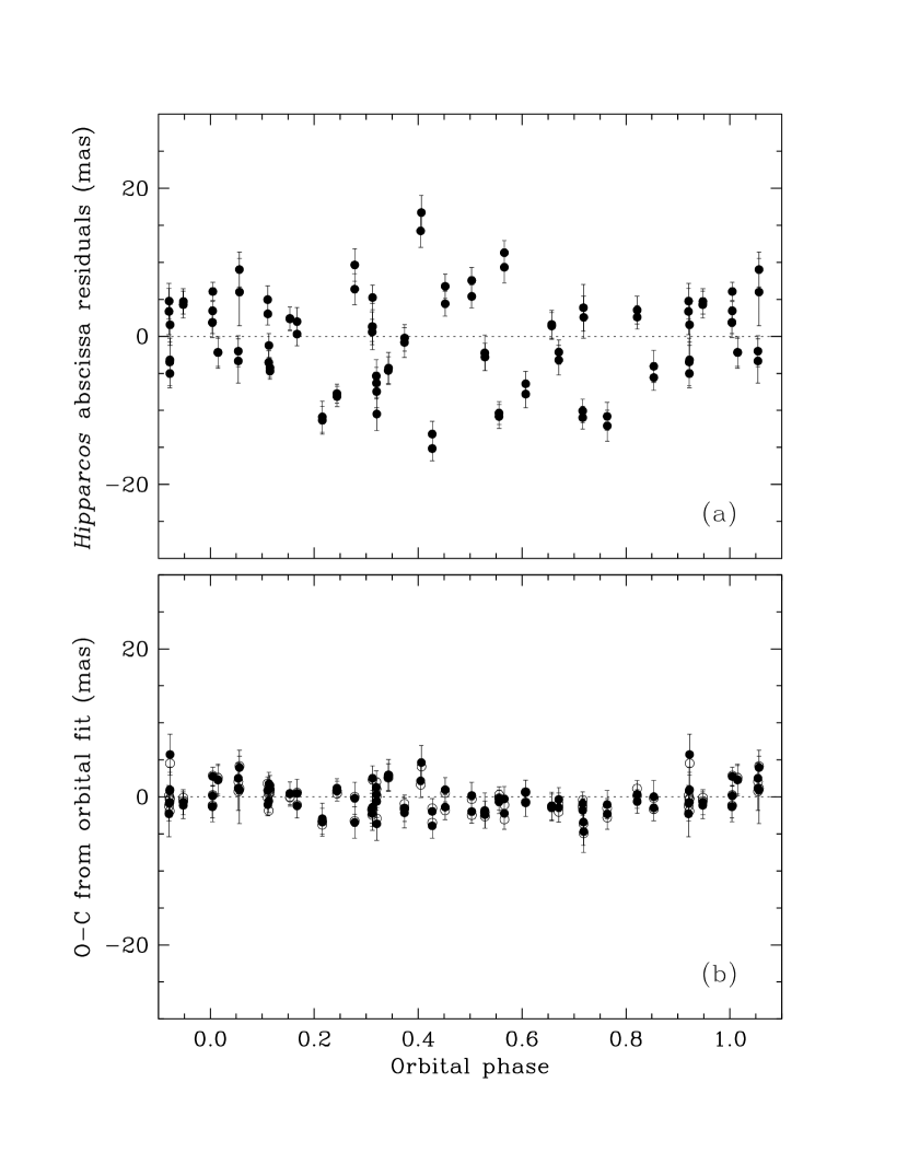
Figure 4.— (a) Abscissa residuals of $\phi$ Her from the Hipparcos mission as a function of orbital phase. These are the residuals from the standard 5-parameter solution as published in the Catalogue (ESA, 1997). The large scatter in excess of the internal errors is an indication that there is unmodeled motion in the system. (b) Filled circles represent the $O\!-\!C$ residuals of the Hipparcos measurements from our orbital fit that combines astrometry and radial velocities. The scatter is now much smaller because the binary motion has been accounted for. The open circles (without the error bars, to avoid clutter) show the $O\!-\!C$ residuals resulting from the orbital fit performed by the Hipparcos team, and are seen to be very similar to ours.

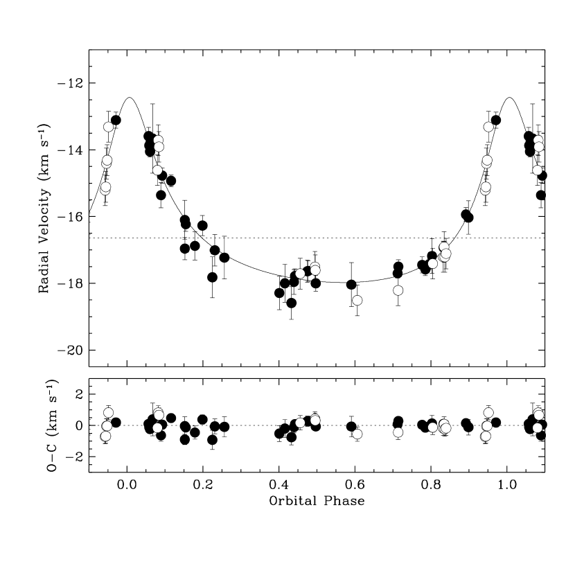
Figure 5.— Radial velocity measurements by Aikman (1976) (filled circles) and Adelman, Gulliver & Rayle (2001) (open circles) along with the computed curve from our combined astrometric-spectroscopic solution. The data by Adelman, Gulliver & Rayle (2001) have been adjusted in this figure for the offset $\Delta RV$ found in our fit (see Table 1). The center-of-mass velocity is indicated with the dotted line. Residuals are shown at the bottom.

Figure 6.— Mass-$M_{V}$ diagram for $\phi$ Her. (a) Model isochrones from the Yonsei-Yale series by Yi et al. (2001) (see also Demarque et al., 2004) for a range of ages, as labeled. Solar composition has been assumed. (b) Best-fitting model that reproduces all six measured properties within their uncertainties (see text). The individual masses and absolute visual magnitudes as well as the combined $U\!-\!B$ and $B\!-\!V$ colors are simultaneously matched to better than 0.4$\sigma$.

Figure 7.— Age and metallicity for all model isochrones by Yi et al. (2001) (see also Demarque et al., 2004) that yield a match to the measured properties of $\phi$ Her (individual masses and absolute visual magnitudes, and combined $U\!-\!B$ and $B\!-\!V$ colors) within the observational errors. The size of the points is an indication of the quality of the agreement, with larger symbols representing a better fit to the data (see text). Solar composition is represented with a dotted line, for reference. The best fit corresponds to [Fe/H] $=-0.03$ and an age of 210 Myr.

References

- Adelman (1984) Adelman, S. J. 1984, A&AS, 55, 479
- Adelman, Adelman & Pintado (2003) Adelman, S. J., Adelman, A. S., & Pintado, O. I. 2003, A&A, 397, 267
- Adelman, Gulliver & Rayle (2001) Adelman, S. J., Gulliver, A. F., & Rayle, K. E. 2001, A&A, 367, 597
- Adelman et al. (2004) Adelman, S. J., Proffitt, C. R., Wahlgren, G. M., Leckrone, D. S., & Dolk, L. 2004, ApJS, 155, 179
- Aikman (1976) Aikman, G. C. L. 1976, Publ. Dom. Astr. Obs., 14, 379
- Babcock (1971) Babcock, H. W. 1971, Carnegie Institution Yearbook, 70, 404
- Demarque et al. (2004) Demarque, P., Woo, J.-H., Kim, Y.-C., & Yi, S. K. 2004, ApJS, 155, 667
- Dolk, Wahlgren & Hubrig (2003) Dolk, L., Wahlgren, G. M., & Hubrig, S. 2003, A&A, 402, 299
- Dworetsky & Budaj (2000) Dworetsky, M. M., & Budaj, J. 2000, MNRAS, 318, 1264
- Dworetsky & Willatt (2006) Dworetsky, M. M., & Willatt, R. 2006, Working Group on Ap Stars at IAU General Assembly in Prague, August 2006, astro-ph/0612432
- ESA (1997) ESA 1997, The Hipparcos and Tycho Catalogues, ESA SP-1200
- Harmanec (1998) Harmanec, P. 1998, A&A, 335, 173
- Høg et al. (2000) Høg, E., Fabricius, C., Makarov, V. V., Urban, S., Corbin, T., Wycoff, G., Bastian, U., Schwekendiek, P., & Wicenec, A. 2000, A&A, 355, L27
- Jancart et al. (2005) Jancart, S., Jorissen, A., Babusiaux, C., & Pourbaix, D. 2005, A&A, 442, 365
- Leushin (1995) Leushin, V. V. 1995, AZh, 72, 543
- Mermilliod & Mermilliod (1994) Mermilliod, J.-C., & Mermilliod, M. 1994, Catalogue of Mean UBV Data on Stars, (New York: Springer)
- Michaud (1970) Michaud, G. 1970, ApJ, 160, 641
- Pourbaix & Jorissen (2000) Pourbaix, D., & Jorissen, A. 2000, A&AS, 145, 161
- Press et al. (1992) Press, W. H., Teukolsky, S. A., Vetterling, W. T., & Flannery, B. P. 1992, Numerical Recipes, (2nd. ed.; Cambridge: Cambridge Univ. Press), 650
- Preston (1974) Preston, G. W. 1974, ARA&A, 12, 257
- van de Kamp (1967) van de Kamp, P. 1967, Principles of Astrometry (San Francisco: W. H. Freeman)
- van Leeuwen & Evans (1998) van Leeuwen, F., & Evans, D. W. 1998, A&AS, 130, 157
- Yi et al. (2001) Yi, S. K., Demarque, P., Kim, Y.-C., Lee, Y.-W., Ree, C. H., Lejeune, T., & Barnes, S. 2001, ApJS, 136, 417
- Zavala et al. (2006) Zavala, R. T., Adelman, S. J., Hummel, C. A., Gulliver, A. F., Caliskan, H., Armstrong, J. T., Hutter, D. J., Johnston, K. J., & Pauls, T. A. 2006, ApJ, in press (astro-ph/0610811)